Statistical physics models for aftershocks and induced seismicity

Abstract

A standard approach to quantifying the seismic hazard is the relative intensity (RI) method. It is assumed that the rate of seismicity is constant in time and the rate of occurrence of small earthquakes is extrapolated to large earthquakes using Gutenberg–Richter scaling. We introduce nowcasting to extend RI forecasting to time-dependent seismicity, for example, during an aftershock sequence. Nowcasting uses ‘natural time’; in seismicity natural time is the event count of small earthquakes. The event count for small earthquakes is extrapolated to larger earthquakes using Gutenberg–Richter scaling. We first review the concepts of natural time and nowcasting and then illustrate seismic nowcasting with three examples. We first consider the aftershock sequence of the 2004 Parkfield earthquake on the San Andreas fault in California. Some earthquakes have higher rates of aftershock activity than other earthquakes of the same magnitude. Our approach allows the determination of the rate in real time during the aftershock sequence. We also consider two examples of induced earthquakes. Large injections of waste water from petroleum extraction have generated high rates of induced seismicity in Oklahoma. The extraction of natural gas from the Groningen gas field in The Netherlands has also generated very damaging earthquakes. In order to reduce the seismic activity, rates of injection and withdrawal have been reduced in these two cases. We show how nowcasting can be used to assess the success of these efforts.

This article is part of the theme issue ‘Statistical physics of fracture and earthquakes’.

1. Introduction

This paper reviews the use of the concepts of natural time and nowcasting in studies of seismicity. The concept of natural time was introduced by Varotsos et al. [1] as a means of studying fracture. Natural time is an event count in place of clock time. For example, it can be the number of small fractures that precede a catastrophic rupture of a brittle material. Varotsos et al. [2] related natural time to the entropy of seismicity. Sarlis et al. [3] and Varotsos et al. [4–6] have suggested that variations of seismicity in natural time are precursory to at least some earthquakes. Varotsos et al. [7] and Sarlis et al. [8] have discussed applications to earthquakes in Japan. Varotsos et al. [9] found precursory behaviour prior to the 2011 Tohoku earthquake in Japan and Sarlis et al. [10] found precursory behaviour prior to the M = 8.2 2017 earthquake in Mexico. A general overview of natural time has been given by Varotsos et al. [11].

In this paper, we consider how the concept of natural time is used to nowcast the occurrence probability for a large earthquake. The basic concept of nowcasting was developed in economic forecasting. The objective is to estimate the current state of the economy using all available data. The gross domestic product is widely accepted as the best measure of economic activity, but accurate estimates have significant delays. Nowcasting uses proxy datasets, for example, unemployment claims and bank deposits [12].

In applying nowcasting to seismicity, the statistical behaviour of small earthquakes is used to infer the statistical behaviour of large earthquakes [13]. Specifically, the event counts of the numbers of small earthquakes between large earthquakes are determined. These are the natural time intervals between the large earthquakes. The statistical distribution of natural time intervals between large earthquakes is determined. The event count since the last large earthquake is used to nowcast the hazard for a large earthquake using the derived statistical distribution.

The extrapolation from small to large earthquake depends on the applicability of Gutenberg–Richter frequency-magnitude statistics. The cumulative number of earthquakes with magnitudes greater than M, N_c, is given by

1.1

where a and b are constants, a is a measure of seismic intensity and the b value is generally near 1. Gutenberg–Richter (GR) scaling can be used to relate the number of large earthquakes with magnitudes greater than M_λ, N_cλ, to the number of small earthquakes with magnitudes greater than M_σ, N_cσ, with the result

1.2

If b = 1 and N_cσ = 10 earthquakes in a year with M_σ≥5, then we can expect to have a M_λ≥7 earthquake in 10 years. The best statistics are obtained if the small earthquake magnitude M_σ is as small as possible; this is the smallest magnitude for which the applicable catalogue is essentially complete. It is assumed that this is the minimum magnitude satisfying the GR statistics given in equation (1.1).

In this paper, we will consider cases in which the seismic intensity, the a value in equation (1.1), is a function of time. One example is in an aftershock sequence, another example is time-dependent induced seismicity. We assume the b value in equations (1.1) and (1.2) is constant and determines the number of large earthquakes, N_cλ, from the number of small earthquakes, N_cσ (natural time). The rate of occurrence of large earthquakes is determined from the observed rate of occurrence of small earthquakes. The rate of occurrence of large earthquakes is the nowcast of a large earthquake.

The use of natural time has several advantages over clock time when applied to earthquakes in a specified region. First, it is not necessary to decluster aftershocks. The natural time count is valid when aftershocks dominate, when background seismicity dominates, and when both contribute. Second, the natural time count is valid when the background rate of seismicity is variable. An example is induced seismicity which can be strongly variable in time. The natural time count defines a constant rate of small earthquake occurrence. This can be extrapolated to large earthquakes using equation (1.2).

Nowcasting using natural time has been applied to global seismicity by Luginbuhl et al. [14]. Many papers discuss whether large earthquakes globally occur randomly in time. Studies in clock time require declustering of aftershocks which is extremely difficult. Declustering is not necessary when clock time is replaced by natural time. To assure high-quality data the Global Centroid Moment Tensor (CMT) catalogue was used beginning in 2004. The completeness magnitude was found to be M_σ = 5.1 so natural time was the event count of M_σ≥5.1 earthquakes. To obtain reasonably good statistics the 197 earthquakes globally with M_λ≥7.0 were considered. The 196 interevent counts of M_σ earthquakes between M_λ earthquakes (natural time intervals) were obtained. The resulting cumulative probability distribution of interevent counts was compared with the best fitting Weibull distribution and the exponent was found to be β = 0.83 ± 0.08. A random distribution would yield β = 1.0. It was concluded that the global distribution of M_λ≥7.0 earthquakes do not occur randomly in natural time.

We use the concept of nowcasting [13] to determine the rate of occurrence of large earthquakes at the present time. We will demonstrate the utility of our approach by forecasting the occurrence of large earthquakes and comparing their occurrence with our forecast. We will consider three applications. The first is to the aftershock sequence of the M = 5.97 Parkfield earthquake on the San Andreas fault. The rate of occurrence of aftershocks is strongly time-dependent. The use of natural time in place of clock time removes this time dependence. The details of our approach are given in §2. The objective is to nowcast the hazard for the occurrence of large aftershocks during the occurrence of the sequence.

Another example of time-dependent seismicity is induced seismicity. Luginbuhl et al. [15] have applied nowcasting to induced earthquakes in Oklahoma and at The Geysers, California. In Oklahoma, the high-pressure injection of large volumes of waste water from the production of hydrocarbons caused a large increase in seismicity from 2013 to 2015. In 2016, Oklahoma regulators ordered a reduction in injection volume. Luginbuhl et al. [15] used nowcasting to monitor the success of the reduction of injection volume in reducing rates of seismicity. In §3 of this paper, we will give a brief update of these results.

Another example of induced seismicity is in the Groningen gas field in The Netherlands. In this case, the induced seismicity is caused by the compaction of the porous reservoir material. The strains associated with localized compaction caused by gas withdrawal results in stresses that load faults leading to earthquakes. A magnitude 3.6 earthquake in August 2012 caused thousands of damage claims and led to a reduction of gas production. Luginbuhl et al. [16] used nowcasting to monitor the success of withdrawal reduction in reducing rates of seismicity. In §4 of this paper, we will give a brief update of these results.

2. Application to Parkfield aftershocks

The rate of aftershock occurrence is strongly time-dependent. The use of natural time in place of clock time removes the time dependence. Aftershocks can result in serious damage and casualties and it is important to provide estimates of the risk as soon as possible after a large earthquake. As a specific example, we will consider the aftershock sequence of the 28 September 2004 Parkfield earthquake. This M = 5.97 mainshock occurred on a well-defined segment of the San Andreas fault in central California. The high-quality seismic network in the vicinity of this mainshock provided a particularly well-documented sequence of aftershocks [17–19]. This is the first application of nowcasting to an aftershock sequence.

The rate at which aftershocks occur decays rapidly after the mainshock. The accepted empirical relation for the decay rate of aftershock activity is the modified form of Omori's Law [20]

2.1

where dN_as/dt is the rate of occurrence of aftershocks with magnitudes greater than M_as, t is the clock time that has elapsed since the mainshock, and τ and c are constant characteristic times that are functions of M_as. It is found that the power p is generally near 1. Setting p = 1 we integrate equation (2.1) to give

2.2

where N_cas is the cumulative number of aftershocks at time t after the mainshock with magnitudes greater than M_as.

Although aftershock sequences are reasonably well approximated by Omori's law, the risk from aftershocks can be quite different for mainshocks with equal magnitudes. The productivity, total number of aftershocks, can vary by a factor of two or more. The constant τ is a measure of the initial productivity but the total productivity also depends on the values of c and p. In some cases, secondary aftershocks are important. A large primary aftershock can have large numbers of secondary aftershocks. An objective of nowcasting is to prescribe the productivity of an aftershock sequence. Using the recorded occurrence of small aftershocks, the expected rate of occurrence of larger aftershocks is nowcast.

In our studies of Parkfield aftershocks, we use the approach given by Shcherbakov et al. [19]. The epicentre of the Parkfield earthquake was at 35.818° N and −120.388° W. The aftershocks are defined to be all earthquakes that occurred in an elliptical region centred at 35.9° N and −120.5° W with radii of 0.4° and 0.15° oriented 137° NW during the 365 days following the mainshock. Clearly, some background seismicity is included. The frequency-magnitude statistics for these earthquakes are given in figure 1. The data were obtained from the Advanced National Seismic System (ANSS) catalogue. An excellent correlation with the GR scaling is obtained for M_as≥1, thus we take M_σ = 1.0.

Figure 1.

The cumulative frequency-magnitude distribution of earthquakes in the study region for 365 days starting 0.1 days after the Parkfield mainshock. The cumulative number of earthquakes per year N_c with magnitudes greater than M are given as a function of M. The best fit of the GR scaling from equation (1.1) is also given, b = 0.96 and a = 4.44. (Online version in colour.)

For our nowcasting study, we will define our natural time to be the event count N_cσ, the cumulative number of small earthquakes with magnitudes greater than M_σ since the starting time. It would appear appropriate to take the starting time to be the time of the mainshock; however, it is difficult to identify many small aftershocks at very early times due to the seismic energy generated by the mainshock. For this reason, we introduce a delay time before the start of our natural time count. We take this delay time to be 0.1 days. We use the subsequent natural time count to nowcast the evolving seismic hazard as the aftershock sequence decays. For the large magnitude values, we select M_λ≥2.5. For the period 0.1 days after the mainshock to 365 days after the mainshock, we plot the cumulative number of large earthquakes, N_cλ, with magnitudes M_λ≥2.5 versus the cumulative number of small earthquakes, N_cσ, with magnitudes M_σ≥1. During this period there were 108 large earthquakes and 3026 small earthquakes. The result is given in figure 2. Also included in this figure is the best least-squares fit to a straight line passing through the origin. Our relationship for the linear fit of N_cλ to N_cσ (natural time) is given in equation (1.2). With N_cλ/N_cσ = 0.0360 from figure 2 and M_λ − M_σ = 1.5, substitution into equation (1.2) gives b = 0.96. This is in excellent agreement with the value b = 0.96 given in figure 1. This agreement supports our assumption that the b-value is constant for the aftershocks.

Figure 2.

Dependence of the cumulative number of large aftershocks with magnitudes greater than M_λ≥2.5, N_cλ, on the cumulative number of small aftershocks with magnitudes greater than M_σ≥1.0, N_cσ (natural time). The data are for 365 days starting 0.1 days after the mainshock. The least-squares linear fit passing through the origin is shown. (Online version in colour.)

In figure 3, we give the cumulative number of small aftershocks, N_cσ, with magnitudes M_σ≥1 (natural time) on clock time in days beginning 0.1 days after the Parkfield mainshock. The temporal decay of aftershock occurrence is clearly shown. We next use the data given in figure 3 to nowcast the occurrence of large aftershocks with M_λ≥2.5 in the sequence. In figure 4, we give the dependence of the cumulative number of large earthquakes, N_cλ, with M_λ≥2.5 on clock time starting 0.1 days after the mainshock. To nowcast these earthquakes we use equation (1.2). We take the values of N_cσ given in figure 3 and multiply by 0.0360. This is the slope of the data in figure 2. The agreement is reasonably good.

Figure 3.

Dependence of the cumulative number of small aftershocks, N_cσ, with magnitudes M_σ≥1.0 (natural time) on clock time, t in days beginning 0.1 days after the mainshock. (Online version in colour.)

Figure 4.

Dependence of the cumulative number of large aftershocks, N_cλ, with magnitudes greater than M_λ≥2.5 on clock time in days beginning 0.1 days after the mainshock. Also included is the nowcast of these earthquakes obtained by multiplying the data given in figure 3 by the slope of the data in figure 2, 0.0360. (Online version in colour.)

At any point in time during the aftershock sequence of a large M_λ≥2.5 occurring is nowcast by the data given in figure 4. We have chosen a relatively small value for M_λ to demonstrate our approach. The probability of occurrence of larger aftershocks, say M_λ≥4, could also have been nowcast during the occurrence of the sequence.

The nowcasting approach illustrated above can be used to nowcast the hazard for the occurrence of large aftershocks. The dependence of the cumulative number of small aftershocks (natural time) on clock time will be sensitive to the productivity of the aftershock sequence. The curve given in figure 3 is a measure of the productivity of the Parkfield aftershocks. At early times, this plot could be used to nowcast the hazard for larger aftershocks at a later time, say at one or 10 days.

3. Induced seismicity in Oklahoma

In recent years, the state of Oklahoma has had a higher rate of seismicity than California [21]. The number of M≥3 earthquakes in Oklahoma per year for the period 2009–2017 is given in figure 5. The increase from 35 M≥3 earthquakes in 2012 to 110 in 2013 to 579 in 2014 and to 903 in 2015 is quite remarkable. That number has since decreased to 624 in 2016 and then to 304 in 2017, which are still high for the region. Oklahoma is in the interior of the North American plate and prior to 2009, the level of seismicity was typical of a plate interior. The recent increase in seismicity cannot be associated with tectonics. It is accepted that the increase in seismicity is caused by the saline waste water injection, primarily water separated directly from oil and gas production.

Figure 5.

Annual numbers of earthquakes in Oklahoma with magnitudes M≥3 for the period 2009–2017. (Online version in colour.)

The total annual volumes of saline water injections in Oklahoma for the period 2011–2016 are given in figure 6. Although the annual injected volumes have changed during this period, the changes in seismicity are much greater. Several authors have correlated the increased seismicity with local injection volumes [22,23].

Figure 6.

Annual volumes of saline water injections in Oklahoma for the period 2011–2016. (Online version in colour.)

Unfortunately, Oklahoma does not have high-resolution catalogues of earthquakes. The network of seismic stations is sparse, although it has recently been improved due to the rapid increase in seismicity. An earthquake catalogue is currently available from the Oklahoma Geological Survey. We have considered the frequency-magnitude statistics for the dataset for the period from 1 January 2013–13 April 2018. The cumulative number of earthquakes, N_c, with magnitudes greater than M are given as a function of M in figure 7. We again correlate the dataset with the GR scaling given in equation (1.1). Good agreement is obtained taking b = 1.52 ± 0.03, this is considerably higher than is usually obtained. The correlation with GR scaling indicates data completeness for about M≥2.75. Thus we take M_σ = 2.75.

Figure 7.

Cumulative frequency-magnitude distribution of earthquakes in Oklahoma for the period 1 January 2013–13 April 2018. The cumulative number of earthquakes per year N_c with magnitudes greater than M are given as a function of M. The straight line correlation is the least-squares fit with the GR scaling from equation (1.1). (Online version in colour.)

In early 2016, Oklahoma regulators called for a 40% reduction in waste water injection. The subsequent reduction has significantly reduced the rate of seismicity in the affected regions [22,23]. Our objective is to demonstrate that nowcasting can quantify the success of the gas withdrawl reduction in reducing the induced seismicity. As in the aftershock example given above, we first nowcast the occurrence of relatively small magnitude earthquakes, in this case M_λ = 4.0, in order to test the success of nowcasting. We then argue that nowcasting can be used to forecast the risk of occurrence of larger induced earthquakes, say M_λ≥6.0. Our results update nowcasting results given by Luginbuhl et al. [15].

Because of the relatively poor resolution of the Oklahoma data, we must select a relatively large M_σ within the completeness range of magnitudes, and we choose M_σ = 2.75. For the large magnitude value, we select M_λ = 4.0. For the period 1 January 2013–13 April 2018, we plot the cumulative number of large earthquakes, N_cλ, with magnitudes M_λ≥4.0 versus the cumulative number of small earthquakes, N_cσ, with magnitudes M_σ≥2.75 (natural time). During this period, there were 68 large earthquakes and 4271 small earthquakes. The result is given in figure 8. Also included in this figure is the best least-squares fit to a straight line passing through the origin. The relationship for the linear fit of N_cλ to N_cσ (natural time) is given in equation (1.2). With N_cλ/N_cσ = 0.0154 from figure 8 and M_λ − M_σ = 1.25, substitution into equation (1.2) gives b = 1.45. This is in good agreement with the value b = 1.52 given in figure 7.

Figure 8.

Dependence of the cumulative number of large earthquakes in Oklahoma with magnitudes M_λ≥4.0, N_cλ, on the cumulative number of small earthquakes with magnitudes M_σ≥2.75, N_cσ (natural time). The data are from the Oklahoma Geological Survey catalogue for the period 1 January 2013–13 April 2018. The least-squares linear fit to the data passing through the origin is also shown. (Online version in colour.)

In figure 9, we give the dependence of the cumulative number of small earthquakes, N_cσ, with magnitudes M_σ≥2.75 (natural time) on the clock time t in days since 1 January 2013. The increase in seismicity early in this period is clearly illustrated. The decrease in seismicity in 2016 and 2017 is also shown. We next use the data given in figure 9 to nowcast the occurrence of large earthquakes in Oklahoma with M_λ≥4.0. In figure 10, we give the dependence of the cumulative number of large earthquakes, N_cλ, with M_λ≥4.0 on clock time t in days since 1 January 2013. To nowcast these earthquakes, we use equation (1.2). We take the value of N_cσ given in figure 9 and multiply by 0.0154. This is the slope of the data in figure 8. The agreement is seen to be quite good.

Figure 9.

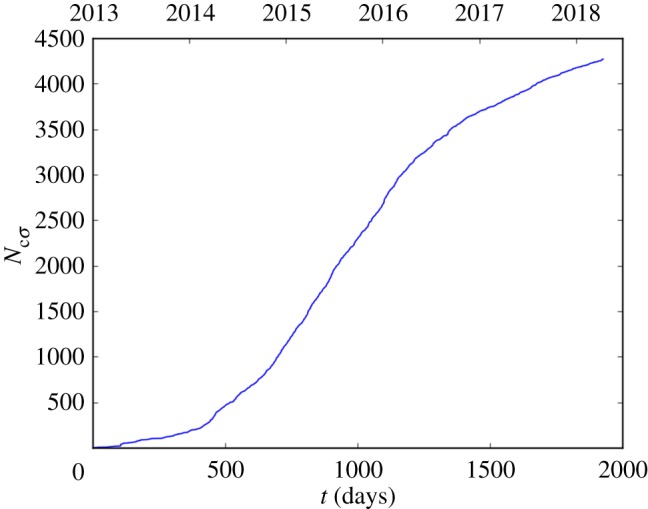
Dependence of the cumulative number of small earthquakes, N_cσ, in Oklahoma with magnitudes M_σ≥2.75 (natural time) on the clock time, t, in days since 1 January 2013. (Online version in colour.)

Figure 10.

Dependence of the cumulative number of large earthquakes in Oklahoma with magnitudes M_λ≥4.0 on clock time, t, in days since 1 January 2013. Also included is the nowcast of these earthquakes obtained by multiplying the data given in figure 9 by the slope of the data given in figure 8, 0.0154. (Online version in colour.)

We have chosen a relatively small value for the large earthquake magnitude, M_λ≥4.0, in order to obtain a sufficiently number of large earthquakes to test the validity of our nowcast. The good correlation given in figure 10 supports extending our nowcast risk of large earthquakes to larger magnitudes.

To illustrate the nowcast approach, we will nowcast the seismic hazard in Oklahoma for 13 April 2018. From figure 9, the rate of occurrence of small earthquakes, M≥M_σ = 2.75, is dN_σ/dt = 0.95 days⁻¹. The mean interevent time for these earthquakes is 1.05 days. The rate of occurrence of large earthquakes, M≥M_λ = 4.0, is dN_λ/dt = 0.95 × 0.0154 = 0.01463 days⁻¹. This is the slope of the line in figure 10 for early 2018. The corresponding interevent time for these earthquakes is 68 days.

Using equation (1.2) we can extend our nowcast to larger earthquakes. Taking M_λ = 5 and b = 1.52, we find dN_λ/dN_σ = 3.8 × 10⁻⁴. With dN_σ/dt = 0.95 days⁻¹, we obtain dN_λ/dt = 3.6 × 10⁻⁴ days⁻¹. The nowcast mean interevent time for a M_λ≥5 earthquake is then 7.6 years.

A primary objective of our study is to quantify the reduction in induced seismicity. This reduction can be obtained directly from figure 10. We compare the rates of seismicity during 2015 and of 13 April 2018 by taking the corresponding slopes of the curve in figure 10. We find that the seismicity has been reduced to 25% of its original value. Our nowcast conclusion is that this reduction is applicable at all magnitudes.

4. Induced seismicity in the Groningen gas field

Another example of induced seismicity is the Groningen natural gas field in The Netherlands [24]. This field was discovered in 1959, production began in 1963, and it is one of the most productive gas fields in Europe. The first induced seismicity occurred in 1991 and the subsequent activity led to the installation of a borehole seismic network in 1995. The data of earthquakes are available from the KNMI catalogue of the Royal Dutch Meteorological Institute. The largest earthquake was the 2012 Huizinge M = 3.6 earthquake on 8 August 2012, which damaged thousands of homes; older homes built with single brick walls were especially vulnerable. The basic hypothesis for the occurrence of the induced seismicity is that stresses resulting from the differential compaction of the reservoir associated with gas withdrawal causes earthquakes on pre-existing faults.

The temporal dependence of natural gas production, which was obtained from the Nederlandse Aardolie Maatschappij (NAM), and the monthly number of induced earthquakes with M≥1.0 for the Groningen gas field are given in figure 11 for the period 1 January 2001–30 June 2018. Peaks of high seismicity appear to follow peaks of high gas production. There is a general increase of seismicity from 2001 to 2014 although there is little variability in the annual gas production. Since 2014 there has been a decrease in seismicity. In response to the damage associated with the 2012 Huizinge M = 3.6 earthquake, the Dutch Government required a reduction in gas production beginning in January 2014. A corresponding decrease in earthquake activity is seen.

Figure 11.

Monthly natural gas production and monthly numbers of earthquakes with M≥1 for the Groningen gas field are given for the period 1 January 2001–30 June 2018. (Online version in colour.)

We consider the frequency-magnitude statistics for the induced seismicity associated with the Groningen gas field for the period 1 January 1996–30 July 2018. The cumulative number of earthquakes, N_c, with magnitudes greater than M are given as a function of M in figure 12. We again correlate the data with GR scaling from equation (1.1). Good agreement is obtained for b = 0.96. The correlation with GR scaling seems to indicate data completeness for about M≥1.0; however, Dost et al. [25] have reported a completeness magnitude of M = 1.5 for the borehole network installed in 1995. Therefore, we will use earthquakes with M≥1.5 in our analysis, and take M_σ = 1.5.

Figure 12.

Cumulative frequency-magnitude distribution of earthquakes in the Groningen region for the period 1 January 1996–30 July 2018. The cumulative number of earthquakes per year, N_c, with magnitudes greater than M are given as a function of M. The straight line correlation is the least-squares fit with the GR scaling from equation (1.1). (Online version in colour.)

An excellent correlation of the data with GR scaling is seen for the magnitude range 1.0 ≤ M ≤ 3.0. An important question is whether this scaling can be extended to higher magnitudes. The application of GR statistics implies that a M = 4.3 earthquake would have been expected during the 22-and-a-half-year period considered. The actual largest earthquake during the period had M = 3.6. However, due to the small number of events, the statistics of the high magnitude rollover are quite uncertain. Zöller & Holschneider [26] have considered the high magnitude statistics and conclude the maximum possible earthquake magnitude in the Groningen gas field is .

We now apply our nowcasting methodology to induced seismicity at the Groningen gas field. This is an update of the results given by Luginbuhl et al. [16]. The frequency-magnitude statistics of the seismicity are given in figure 12. As the smallest magnitude for which we expect to give catalogue completeness, we take M_σ = 1.5. For the large magnitude, we choose M_λ = 2.5. For the period of 1 January 1996–30 July 2018, we plot the cumulative number of large earthquakes, N_cλ, in the study region with magnitudes M_λ≥2.5 versus the cumulative number of small earthquakes, N_cσ, with M_σ≥1.5 (natural time). The results are given in figure 13; there are 36 large earthquakes and 314 small earthquakes. Also included in this figure is the best least-squares fit to a straight line passing through the origin. Our relationship for the linear fit of N_cλ to N_cσ (natural time) is given in equation (1.2). With N_cλ/N_cσ = 0.1235 from figure 13 and M_λ − M_σ = 1.0, substitution into equation (1.2) gives b = 0.91. This is in quite good agreement with the value b = 0.96 given in figure 12.

Figure 13.

Dependence of the cumulative number of large earthquakes in the Groningen gas field with magnitudes M_λ≥2.5, N_cλ, on the cumulative number of small earthquakes, N_cσ (natural time), with magnitudes M_σ≥1.5 for the period 1 January 1996–30 July 2018. The data are from the KNMI catalogue. The least-squares linear fit to the data passing through the origin is also shown. (Online version in colour.)

In figure 14, we give the dependence of the cumulative number of small earthquakes, N_cσ, with M_σ≥1.5 (natural time) on clock time in days from 1 January 1996–30 July 2018. There is a systematic increase in the rate of seismicity until 2014 and subsequently a small decrease. In figure 15, we give the dependence of the cumulative number of large earthquakes N_cλ with M_λ≥2.5 on clock time in days from 1 January 1996–30 July 2018. To nowcast the earthquakes in figure 15 we use equation (1.2), we take the values of N_cσ given in figure 14 and multiply by 0.1235. This is the slope of the data in figure 13, and the agreement is quite good.

Figure 14.

Dependence of the cumulative number of small earthquakes, N_cσ, in the Groningen region with magnitudes M_σ≥1.5 (natural time) on clock time, t, in days since 1 January 1996. (Online version in colour.)

Figure 15.

Dependence of the cumulative number of large earthquakes in the Groningen region with magnitudes M_λ≥2.5, N_cλ, on clock time t in days since 1 January 1996. Also included is the nowcast of these earthquakes obtained by multiplying the data given in figure 13 by the slope of the data in figure 14, 0.1235. (Online version in colour.)

There are similarities between the data for Oklahoma and Groningen, but there are some important differences. The quality of the seismic data at Groningen is clearly superior leading to a much lower M_σ. However, the agreement between the frequency-magnitude statistics and GR scaling is better for Oklahoma, as can be seen by comparing figure 7 with figure 12. There appears to be a rollover for larger magnitudes for the Groningen data. If this rollover is real, it significantly reduces the risk of larger earthquakes at Groningen. We will consider the implications of this deviation from GR scaling on our nowcasting approach.

We will nowcast the seismic hazard at Groningen for 30 July 2018. From figure 14 the rate of occurrence of small earthquakes with M≥M_σ = 1.5 is dN_σ/dt = 0.0526 days⁻¹. The mean interevent time for the small earthquakes is 19 days. The rate of occurrence of large earthquakes with M≥M_λ = 2.5 is dN_λ/dt = 0.0526 × 0.1235 = 6.5 × 10⁻³ days⁻¹. This is the slope of the line in figure 15 for 2017 and the first half of 2018. The nowcasted interevent time for these earthquakes is 154 days.

Our nowcast of a M_λ≥2.5 earthquakes is expected to be valid since GR scaling is valid as seen in figure 12. However, nowcasting a larger earthquake presents a problem because GR scaling may not be valid. Taking M_λ = 3.5 and b = 0.96 from figure 12, we find from equation (1.2) that dN_λ/dN_σ = 0.01202. With dN_σ/dt = 0.0526 days⁻¹, we obtain dN_λ/dt = 6.32 × 10⁻⁴ days⁻¹. The nowcasted interevent time at the present time for a M_λ≥3.5 earthquake is 4.3 years.

Alternatively, we can nowcast this larger earthquake using the frequency-magnitude scaling from figure 12. From this figure, the rate of occurrence of a M_λ≥3.5 earthquake is 0.0794 per year for the full timespan. Similarly, the rate of occurrence of a M_σ≥1.5 is 12.6 per year. This gives dN_λ/dN_σ = 6.3 × 10⁻³. With dN_σ/dt = 0.0526 days⁻¹, we obtain dN_λ/dt = 3.3 × 10⁻⁴ days⁻¹. Using this approach, the present nowcasted interevent time for a M_λ≥3.5 earthquake is 8.3 years. We see that the nowcast hazard is about a factor of two lower using the observed scaling versus the GR scaling.

5. Discussion

If the seismicity in a region is statistically stationary (not a function of time) the mean intervals between events with magnitudes greater than a specified value can be obtained directly from the form of GR scaling given in equation (1.2). If b = 1, the mean interevent time increases by a factor of 10 for each unit change of magnitude. If there are 10 M≥3 earthquakes per year in the region, on average there will be one M≥4 earthquake per year, a mean interval of 10 years for a M≥5 earthquake, etc. This approach is, in fact, useful to provide a measure of the seismic hazard. However, seismic activity is in general time-dependent; aftershocks are a prime example. In this paper, we illustrate how the concept of seismic nowcasting can be used to provide estimates of the statistical hazard at the present time. The method can be applied when the seismicity is time-dependent, for example during an aftershock sequence.

Nowcasting uses the concept of natural time, which is an event count. For seismic nowcasting the event count is the number of earthquakes above a minimum earthquake magnitude M≥M_σ, N_cσ. The objective is to relate the natural time count to the number of large earthquakes with magnitude M≥M_λ, N_cλ. This association requires the validity of a frequency-magnitude scaling throughout the range of magnitudes considered. If the scaling is GR then the relationship is given by equation (1.2), but GR scaling is not required for nowcasting seismicity. Data on frequency-magnitude scaling provide the network sensitivity and the smallest magnitude for which the seismic catalogue is complete.

If seismicity is time-independent the nowcasting method can be used in clock time to forecast the future seismic hazard. An example of this approach, known as a relative intensity (RI) forecast, has been given by Holliday et al. [27]. If seismicity is time-dependent the nowcasting method cannot be used to forecast the future seismic hazard since the future level of seismic activity is not known.

In this paper, we illustrate the application of nowcasting with three examples. We first consider an aftershock sequence and choose the September 2004 Parkfield earthquake on the San Andreas fault in California. This aftershock sequence is chosen because of the existence of an excellent catalogue of aftershocks. Empirically, aftershocks correlate with the GR frequency-magnitude scaling as given in equation (1.1), Omori's Law as given in equation (2.1) for their temporal decay, and a modified form of Båth's Law [28]. In the modified form of Båth's Law, the largest aftershock magnitude consistent with GR scaling, M*, is determined by the intersection of the scaling law with N_c = 1. The difference between this magnitude and the mainshock magnitude M_ms, ΔM* = M_ms − M* has considerable variation. Shcherbakov & Turcotte [28] found values from ΔM* = 0.6 to 1.5 for 10 large California earthquakes. Thus the number of aftershocks for earthquakes of the same magnitude can vary by an order of magnitude. The value of ΔM* is a measure of aftershock productivity. From figure 1, we see that ΔM* = 5.97 − 4.6 = 1.37 for the Parkfield aftershock sequence. One objective of nowcasting is to obtain a real-time measure of aftershock productivity. The nowcast of the numbers of small and large aftershocks are given in figures 3 and 4.

We also consider two examples of the nowcasting of induced earthquakes. The first is the induced seismicity caused by petroleum waste water injection in Oklahoma. The second is the induced seismicity caused by gas production in the Groningen gas field, The Netherlands. In order to reduce rates of seismicity the rate of waste water injection was reduced in Oklahoma and the rate of gas withdrawal was reduced in The Netherlands. We have shown how nowcasting can be used to quantify the effectiveness of these measures. The reduction in Oklahoma is illustrated in figure 10 and the reduction in Groningen is illustrated in figure 15. Clearly, the reduction has been more effective in Oklahoma than in Groningen.

Data accessibility

Data for the Parkfield analysis were obtained from the ANSS global composite catalogue, available at http://www.quake.geo.berkeley.edu/anss/catalog-search.html. Data for the Oklahoma analysis were obtained from the Oklahoma Geological Survey earthquake catalogue, available at http://www.ou.edu/content/ogs/research/earthquakes/catalogs.html, and from the Oklahoma Corporation Commission, Oil and Gas Division, available at http://www.occeweb.com/og/ogdatafiles2.htm. Data for the Groningen analysis were obtained from the KNMI catalogue of the Royal Dutch Meteorological Institute, available at http://rdsa.knmi.nl/dataportal, and from the NAM, available at http://www.namplatform.nl/feiten-en-cijfers/gaswinning.

Authors' contributions

J.B.R. conceived of the nowcasting method using natural time. D.L.T. designed the study and helped in interpretation of the data and drafting the manuscript. M.L. acquired the data, carried out the statistical analysis and drafted the manuscript. All authors gave final approval for publication.

Competing interests

There are no competing interests for this manuscript.

Funding

M.L. and J.B.R. were funded by a grant from the US Department of Energy to the University of California, Davis, DoE grant no. DE- SC0017324.

References

- 1.Varotsos PA, Sarlis NV, Skordas ES. 2002. Long-range correlations in the electric signals that precede rupture. Phys. Rev. E 66, 011902 ( 10.1103/PhysRevE.66.011902) [DOI] [PubMed] [Google Scholar]
- 2.Varotsos PA, Sarlis NV, Tanaka HK, Skordas ES. 2005. Some properties of the entropy in the natural time. Phys. Rev. E 71, 032102 ( 10.1103/physreve.71.032102) [DOI] [PubMed] [Google Scholar]
- 3.Sarlis N, Skordas E, Varotsos P. 2010. Nonextensivity and natural time: the case of seismicity. Phys. Rev. E 82, 021110 ( 10.1103/PhysRevE.82.021110) [DOI] [PubMed] [Google Scholar]
- 4.Varotsos P, Sarlis N, Skordas E. 2011. Scale-specific order parameter fluctuations of seismicity in natural time before mainshocks. EPL (Europhysics Letters) 96, 59002 ( 10.1209/0295-5075/96/59002) [DOI] [Google Scholar]
- 5.Varotsos P, Sarlis NV, Skordas ES, Uyeda S, Kamogawa M. 2011. Natural time analysis of critical phenomena. Proc. Natl Acad. Sci. USA 108, 11 361–11 364. ( 10.1073/pnas.1108138108) [DOI] [PMC free article] [PubMed] [Google Scholar]
- 6.Varotsos PA, Sarlis NV, Skordas ES. 2017. Identifying the occurrence time of an impending major earthquake: a review. Earthquake Sci. 30, 209–218. ( 10.1007/s11589-017-0182-7) [DOI] [Google Scholar]
- 7.Varotsos PA, Sarlis NV, Skordas ES. 2014. Study of the temporal correlations in the magnitude time series before major earthquakes in Japan. J. Geophys. Res. Space Phys. 119, 9192–9206. ( 10.1002/2014JA020580) [DOI] [Google Scholar]
- 8.Sarlis NV, Skordas ES, Varotsos PA, Nagao T, Kamogawa M, Uyeda S. 2015. Spatiotemporal variations of seismicity before major earthquakes in the Japanese area and their relation with the epicentral locations. Proc. Natl Acad. Sci. USA 112, 986–989. ( 10.1073/pnas.1422893112) [DOI] [PMC free article] [PubMed] [Google Scholar]
- 9.Varotsos PA, Sarlis NV, Skordas ES, Lazaridou-Varotsos MS. 2017. Mw 9 Tohoku earthquake in 2011 in Japan: precursors uncovered by natural time analysis. Earthquake Sci. 30, 183–191. ( 10.1007/s11589-017-0189-0) [DOI] [Google Scholar]
- 10.Sarlis NV, Skordas ES, Varotsos PA, Ramírez-Rojas A, Flores-Márquez EL. 2018. Natural time analysis: on the deadly Mexico M8. 2 earthquake on 7 September 2017. Phys. A Stat. Mech. Appl. 506, 625–634. ( 10.1016/j.physa.2018.04.098) [DOI] [Google Scholar]
- 11.Varotsos PA, Sarlis NV, Skordas ES. 2011. Natural time analysis: the new view of time: precursory seismic electric signals, earthquakes and other complex time series. Berlin, Germany: Springer Science & Business Media. [Google Scholar]
- 12.Giannone D, Reichlin L, Small D. 2008. Nowcasting: the real-time informational content of macroeconomic data. J. Monetary Econ. 55, 665–676. ( 10.1016/j.jmoneco.2008.05.010) [DOI] [Google Scholar]
- 13.Rundle JB, Turcotte DL, Donnellan A, Grant Ludwig L, Luginbuhl M, Gong G. 2016. Nowcasting earthquakes. Earth Space Sci. 3, 480–486. ( 10.1002/2016EA000185) [DOI] [Google Scholar]
- 14.Luginbuhl M, Rundle JB, Turcotte DL. 2018. Natural time and nowcasting earthquakes: are large global earthquakes temporally clustered? Pure Appl. Geophys. 175, 661–670. ( 10.1007/s00024-018-1778-0) [DOI] [Google Scholar]
- 15.Luginbuhl M, Rundle JB, Hawkins A, Turcotte DL. 2018. Nowcasting Earthquakes: a comparison of induced earthquakes in Oklahoma and at The Geysers, California. Pure Appl. Geophys. 175, 49–65. ( 10.1007/s00024-017-1678-8) [DOI] [Google Scholar]
- 16.Luginbuhl M, Rundle JB, Turcotte DL. 2018. Natural time and nowcasting induced seismicity at the Groningen gas field in the Netherlands. Geophys. J. Int. 215, 753–759. ( 10.1093/gji/ggy315) [DOI] [Google Scholar]
- 17.Bakun W. et al. 2005. Implications for prediction and hazard assessment from the 2004 Parkfield earthquake. Nature 437, 969–974. ( 10.1038/nature04067) [DOI] [PubMed] [Google Scholar]
- 18.Langbein J. et al. 2005. Preliminary report on the 28 September 2004, M 6.0 Parkfield, California Earthquake. Seismol. Res. Lett. 76, 10–26. ( 10.1785/gssrl.76.1.10) [DOI] [Google Scholar]
- 19.Shcherbakov R, Turcotte DL, Rundle JB. 2006. Scaling properties of the Parkfield aftershock sequence. Bull. Seismol. Soc. Am. 96, S376–S384. ( 10.1785/0120050815) [DOI] [Google Scholar]
- 20.Utsu T. 1961. A statistical study on the occurrence of aftershocks. Geophys. Mag. 30, 521–605. [Google Scholar]
- 21.Walsh FR, Zoback MD. 2015. Oklahoma's recent earthquakes and saltwater disposal. Sci. Adv. 1, e1500195 ( 10.1126/sciadv.1500195) [DOI] [PMC free article] [PubMed] [Google Scholar]
- 22.Langenbruch C, Zoback MD. 2016. How will induced seismicity in Oklahoma respond to decreased saltwater injection rates? Sci. Adv. 2, e1601542 ( 10.1126/sciadv.1601542) [DOI] [PMC free article] [PubMed] [Google Scholar]
- 23.van der Baan M, Calixto FJ. 2017. Human-induced seismicity and large-scale hydrocarbon production in the USA and Canada. Geochem. Geophys. Geosyst. 18, 2467–2485. ( 10.1002/2017GC006915) [DOI] [Google Scholar]
- 24.van Thienen-Visser K, Breunese JN. 2015. Induced seismicity of the Groningen gas field: history and recent developments. Leading Edge 34, 664–671. ( 10.1190/tle34060664.1) [DOI] [Google Scholar]
- 25.Dost B, Goutbeek F, van Eck T, Kraaijpoel D. 2012. Monitoring induced seismicity in the north of the Netherlands: status report 2010. KNMI Scientific report, 2012–2003.
- 26.Zöller G, Holschneider M. 2016. The maximum possible and the maximum expected earthquake magnitude for production-induced earthquakes at the gas field in Groningen, the Netherlands. Bull. Seismol. Soc. Am. 106, 2917–2921. ( 10.1785/0120160220) [DOI] [Google Scholar]
- 27.Holliday JR, Chen C-C, Tiampo KF, Rundle JB, Turcotte DL, Donnellan A. 2007. A relm earthquake forecast based on pattern informatics. Seismol. Res. Lett. 78, 87–93. ( 10.1785/gssrl.78.1.87) [DOI] [Google Scholar]
- 28.Shcherbakov R, Turcotte DL. 2004. A modified form of Bath's law. Bull. Seismol. Soc. Am. 94, 1968–1975. ( 10.1785/012003162) [DOI] [Google Scholar]
Associated Data
This section collects any data citations, data availability statements, or supplementary materials included in this article.
Data Availability Statement