

Abstract
The (global) optimization of energy systems, commonly characterized by high-fidelity and large-scale complex models, poses a formidable challenge partially due to the high noise and/or computational expense associated with the calculation of derivatives. This complexity is further amplified in the presence of multiple conflicting objectives, for which the goal is to generate trade-off compromise solutions, commonly known as Pareto-optimal solutions. We have previously introduced the p-ARGONAUT system, parallel AlgoRithms for Global Optimization of coNstrAined grey-box compUTational problems, which is designed to optimize general constrained single objective grey-box problems by postulating accurate and tractable surrogate formulations for all unknown equations in a computationally efficient manner. In this work, we extend p-ARGONAUT towards multi-objective optimization problems and test the performance of the framework, both in terms of accuracy and consistency, under many equality constraints. Computational results are reported for a number of benchmark multi-objective problems and a case study of an energy market design problem for a commercial building, while the performance of the framework is compared with other derivative-free optimization solvers.
Keywords: Derivative-free optimization, Grey/black-box optimization, Multi-objective optimization, Energy systems engineering
1. Introduction
Energy systems are characterized by a large and diverse number of components in which they form an integrated complex multi-scale network (Floudas et al., 2016). Mathematical models defining such complex systems generally include expensive finite-elements, a large number of partial differential equations (PDEs) and high-fidelity models. The global optimization of these systems using deterministic methods is often challenging since the calculation of the derivatives can be subject to high noise and/or computational expense. These characteristics are displayed by many systems in the fields of engineering and sciences, and commonly referred to as “grey-box” or “black-box” problems, where the system relies on expensive simulations, proprietary codes or input-output data (Boukouvala et al., 2016). A general constrained nonlinear grey-box problem is mathematically defined in Eq. 1:
| (1) |
where n represents the number of continuous decision variables with known lower and upper bounds [xL, xU] and set k ∈ {1,…,K} represents the constraints with known closed-form equations. The mathematical expressions defining the objective, f(x), and the constraints, represented by set m ∈ {1,…,M}, are not explicitly available as a function of the continuous decision variables. However, the values of these unknown formulations can be retrieved as outputs of the problem simulator, which is typically computationally expensive. In the problem of interest, “unknown” strictly refers to the mathematical expression of an equation (objective or constraints) in terms of x, and the cardinality of set should be known a priori.
The complexity of such multi-scale models is further amplified in the presence of multiple competing objectives, such as economic and environmental objectives that are commonly associated with the optimal design of energy systems. In this case, it is not possible to locate a unique optimal solution since there are trade-offs between these conflicting objectives. This class of optimization problems are handled via multi-objective optimization (MOO), of which the goal is to find the best set of decisions that will simultaneously optimize multiple objectives in such a way that the solutions cannot be improved without degrading at least one of the other objectives (Miettinen, 1998). In other words, the goal of MOO is to derive a set of trade-off optimal solutions, known as the Pareto-optimal solutions, that the decision makers can choose from, depending on their preferences. The general form of MOO problems is presented in Eq. 2:
| (2) |
where is a non-empty feasible region, X ⊂ ℝn.
While several methodologies exist in the open literature for MOO, we only consider the ones that are linked to population-based and surrogate-based algorithms. Meta-heuristic (population-based) algorithms are advantageous since they do not require any reformulations, such as converting the multi-objective problem into a set of single-objective sub-problems. These can simultaneously deal with a set of possible solutions without requiring series of separate runs, thus enabling the direct investigation of the multi-objective problem (Coello et al., 2007). As a result, population-based algorithms have been a popular choice among many researchers for the MOO of various systems, including truss design (Ray et al., 2001), thermal system design (Toffolo and Lazzaretto, 2002), environmental economic power dispatch (Gong et al., 2010; Wang and Singh, 2007), beam design (Sanchis et al., 2008), water distribution network design (di Pierro et al., 2009) and more recently the MOO of zeolite framework determination (Abdelkafi et al., 2017). In addition to these, the books by Rangaiah and Bonilla-Petriciolet (2013), and Coello et al. (2007) demonstrate a plethora of applications of evolutionary algorithms to numerous MOO problems.
Even though the population-based algorithms are widely studied in the open literature, their application to grey/black-box problems are rather limited. There are two main reasons for this: (1) most existing algorithms consider the box-constrained problem or handle general constraints via penalty functions, where the system is being continuously treated as a black-box; (2) stochastic algorithms typically require a large number of function calls to reach the global optimality, which can be computationally prohibitive for expensive simulations. Several researchers have focused on hybrid implementations of surrogate modeling with stochastic algorithms to overcome such problems. Datta and Regis (2016) have proposed a surrogate-assisted evolution strategy, which makes use of cubic radial basis surrogate models to guide the evolution strategy for the optimization of multi-objective black-box functions that are subject to black-box inequality constraints. Likewise, Bhattacharjee et al. (2016) have used a well-known evolutionary algorithm, NSGA-II, as the baseline algorithm while using multiple local surrogates of different types to represent the objectives and the constraints.
Surrogate-based approaches, where the objectives and the grey/black-box constraints are approximated with simple tractable models, have also been investigated in the open literature in conjunction with derivative-free algorithms. Singh et al. (2014) have proposed the Efficient Constrained Multi-objective Optimization (ECMO) algorithm to solve computer-intensive constrained multi-objective problems using Kriging models for the objectives and the constraints. They make use of the hypervolume-based Probability of Improvement (PoI) criterion to handle multiple objectives along with the Probability of Feasibility (PoF) criterion to handle computationally expensive constraints and solve the final formulation using MATLAB’s fmincon optimizer. Feliot et al. (2017) have used an expected hypervolume improvement sampling criterion in their Bayesian Multi-Objective Optimization (BMOO) framework, where the nonlinear implicit constraints and the black-box objectives are handled via extended domination rule. In this algorithm, the authors use sequential Monte Carlo sampling technique for the computation and optimization of the expected improvement criterion. Martínez-Frutos and Herrero-Pérez (2016) have introduced the Kriging-based Efficient Multi-Objective Constrained Optimization (KEMOCO) algorithm that uses a kriging-based infill sampling strategy with DIRECT algorithm for constrained MOO of expensive black-box simulations. They combine the expected hypervolume improvement and the PoF to obtain the Pareto-front with minimum number of samples. Regis (2016) has presented Multi-Objective Constrained Stochastic optimization using Response Surfaces (MOCS-RS) framework where the author uses radial basis surrogates as approximations for the objective and constraint functions. A more detailed overview on the existing methods for using surrogates in computationally expensive MOO can be found in Tabatabaei et al. (2015).
In this paper, we implement a hybrid methodology that performs global parameter estimation coupled with k-fold cross-validation for individualized surrogate model identification on each unknown formulation (objective and constraints). Specifically, we employ the parallel AlgoRithms for Global Optimization of coNstrAined grey-box compUTational problems (p-ARGONAUT) algorithm (Beykal et al., 2018; Boukouvala and Floudas, 2017; Boukouvala et al., 2017) to explore the effect of maximizing the connection between surrogate model identification and deterministic global optimization in MOO problems. Our framework is tailored to solve high-dimensional general constrained grey-box problems, which contains several features including, adaptive parallel sampling, variable screening, exploration and validation of the best surrogate formulation for each unknown equation, and global optimization of the proposed surrogate formulations for improved solutions. The parallel algorithm is tested on three constrained MOO benchmark problems as well as a more complex case study of an energy market design problem for a commercial building. By implementing the ε-constraint method to convert the MOO problem into series of single-objective optimization sub-problems, p-ARGONAUT is employed to globally optimize the resulting constrained grey-box problems.
The paper is structured as follows. Section 2 provides the details on our framework to globally optimize high-dimensional general constrained grey-box computational problems that benefits from high-performance computing for maximal computational efficiency. In Section 3.1, we provide an overview of the methodology we employed to convert MOO into a series of single-objective optimization sub-problems, namely the ε-constraint method. Moreover, in Section 3.2, we solve a motivating example to show the details on p-ARGONAUT iterations. Finally, the details of the computational studies are provided in Section 4 followed by the results and concluding remarks in Sections 5 and 6, respectively.
2. Parallel AlgoRithms for Global Optimization of coNstrAined grey-box compUTational problems (p-ARGONAUT)
p-ARGONAUT is an extension of the ARGONAUT algorithm (Boukouvala and Floudas, 2017; Boukouvala et al., 2017) which uses high-performance parallel computing to globally optimize high-dimensional general constrained grey-box problems. It incorporates the information provided in the form of input-output data with known equations to formulate a nonconvex nonlinear programming (NLP) problem, which is later solved to global optimality using deterministic methods. p-ARGONAUT starts with bounds tightening and parallel sampling, continues with variable selection and extensive exploration of possible surrogate formulations for each unknown equation via global optimization of the parameter estimation problem, and ends with new sample identification for the next iteration through local and global optimization of the constrained grey-box NLP. The iterative algorithmic flowchart for p-ARGONAUT is given in Fig. 1.
Fig. 1.
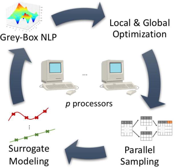
Algorithmic flowchart of p-ARGONAUT where 3 main stages of the framework is performed on multiple processors, namely the sampling, surrogate modeling and the optimization.
The algorithm requires an initial input from the user, regarding the important parameters characterizing the constrained grey-box problem. These are the number of input variables, number of unknown constraints, number of known constraints, as well as their analytical form, and the finite bounds on the input variables. In the presence of any known equations, p-ARGONAUT will use optimality-based-bound-tightening (OBBT) to further tighten the finite bounds on the input variables and perform Latin Hypercube Sampling for the initial design of experiments. Later, given that p processors are available, p-ARGONAUT can partition the initial sampling set into p different subsets, and run the problem simulation in parallel to collect the outputs. This stage is critical to computationally expensive constrained grey-box problems since the computational cost of repetitive function calls can burden the overall optimization process. As a result, parallelizing sample collection over multiple processors improves the computational efficiency of the overall framework significantly.
After this stage, the algorithm proceeds with variable selection and surrogate model identification, in which the parameters of possible surrogate formulations are globally optimized, and the postulated formulations are cross-validated for superior accuracy. This procedure is iteratively done for all surrogate functions present in the p-ARGONAUT’s library by default, to explore the best possible surrogate representing each unknown equation with minimum average cross-validation error. Moreover, one of the most important features of p-ARGONAUT is its ability to take advantage of any a priori knowledge on the nonlinearity of unknown formulations. In that case, it is possible to fix the surrogate function type for any unknown equation at the beginning of the algorithm. Then, only the parameters of the specified surrogate type are globally determined.
In the final stage, p-ARGONAUT formulates a nonconvex constrained NLP using the proposed surrogate approximations for the objective and for the unknown constraints as well as with the known information provided at the beginning of the algorithm. This hybrid NLP is then solved to local optimality with multiple starting points using CONOPT (Drud, 1994) and to global optimality using the deterministic global solver ANTIGONE (Misener and Floudas, 2012; Misener and Floudas, 2013, 2014). The solution to these series of optimization problems become the new sampling points for the next iteration and the framework proceeds with updating the surrogate models as well as locating new samples until convergence.
Like in the sampling phase, it is also possible to benefit from high-performance computing at the model identification stage and in the optimization stage. During the model identification process, each unknown equation is assumed to have a unique and independent form with respect to each other. Hence, parameter estimation, model identification and cross-validation can be done on multiple processors. Similarly, in the optimization step, each optimization problem is independent from each other and can be solved in parallel to maximize the computational efficiency.
It is important to state that the performance and computational requirements of the algorithm is affected by the dimensionality of the grey/black-box problem and the number and type of constraints. We have previously shown that the algorithm can locate the global optimal solution for single-objective benchmark problems with up to 100 variables (Boukouvala and Floudas, 2017). We have also previously tested the p-ARGONAUT framework on a complex case study of oil production optimization via controlling the pressure in injection and production wells for a water-flooding process (Beykal et al., 2018; Sorek et al., 2017). In this case study, the true global solution was unknown, but we have shown that p-ARGONAUT can provide consistent improved solutions to problems with several thousand grey-box constraints. In this work, we further expand the applicability of our framework on MOO problems and test the performance of the framework on several benchmark studies as well as on a case study of multi-objective energy systems design problem, which is subject to equality constraints. Finally, it is important to note that even though our method can guarantee ε-global optimality of the surrogate-based formulation by using a global optimization solver (ANTIGONE), there is no theoretical guarantee for global optimality of the original grey/black-box problem, due to the fact that we make no assumptions regarding the smoothness or convexity of the objective or constraints of the problem.
3. Methods
3.1. Multi-Objective Optimization Using ε-Constraint Method
The ε-constraint method is introduced by Clark and Westerberg (1983) to convert multi-objective design problems into series of single-objective sub-problems. Consider an optimization problem given in the form of Eq. 2 with only 2 objectives, i.e. N = 2. The main idea behind ε-constraint method is to discretize the objective space into smaller sections while obtaining the optimal solution at each discretization point to generate the Pareto-optimal curve. The discretization is done by moving one of the objectives into the constraints set while setting an upper bound (ε) on the new constraint. This simply converts the MOO into a single-objective optimization problem with an added expense of a single inequality constraint, as shown in Eq. 3.
| (3) |
The lower and upper bounds, [εL, εU] on the discretization points can be derived by minimizing each of the objectives independently. The optimal solution resulting from the minimization of the first objective, , mathematically formulated in Eq. 4, will give the maximum value of the second objective, , provided that increasing the value of f2 beyond this maximum value will not affect the value of f1. Thus, εU will be equal to .
| (4) |
Similarly, the lower bound on εL is derived by minimizing f2 as a single-objective optimization problem. The optimal solution to this problem, , gives the minimum possible value of f2, which is also the minimum value of ε. Hence, εL will be equal to . Using these values of [εL, εU], the objective region can now be divided into N equal intervals as follows:
| (5) |
Then, the final optimization problem becomes:
| (6) |
Although, we have provided a walk-through for problems with two objectives, the ε-constraint method is a general partitioning strategy. For a system with N competing objectives, a similar procedure will be followed as the one shown in Eq. 3, creating a minimization problem with N − 1 constraints, which are added to the initial problem formulation. Then, the lower and upper bounds on ε for the partitioned objectives, [εL,, εU]1 ×…× [εL,, εU]N−1, will define the boundaries of a Pareto-optimal surface when N = 3 and a Pareto-optimal polyhedron when N ≥ 3.
3.2. Motivating Example
In this section, we demonstrate the key steps of p-ARGONAUT on a motivating example and show how the framework models the system dynamics as well as the solution of the postulated surrogates to global optimality. We consider the following multi-objective problem:
| (7) |
• Step 1: Dissect the objective space using Eq. 5
As shown in Section 3.1, minimization of the first and second objectives gives the upper and lower bounds for the ε parameter (ε ∈ [4,50]), respectively. Within these bounds, we dissect the objective space to 30 equal points using Eq. 5. Table 1 summarizes the values of ε corresponding to each point.
Table 1.
Resulting values of the from discretization of the objective space into 30 points.
| Point Number | ε | Point Number | ε | Point Number | ε |
|---|---|---|---|---|---|
| 1 | 50 | 11 | 34.13793 | 21 | 18.27586 |
| 2 | 48.41379 | 12 | 32.55172 | 22 | 16.68966 |
| 3 | 46.82759 | 13 | 30.96552 | 23 | 15.10345 |
| 4 | 45.24138 | 14 | 29.37931 | 24 | 13.51724 |
| 5 | 43.65517 | 15 | 27.79310 | 25 | 11.93103 |
| 6 | 42.06897 | 16 | 26.20690 | 26 | 10.34483 |
| 7 | 40.48276 | 17 | 24.62069 | 27 | 8.75862 |
| 8 | 38.89655 | 18 | 23.03448 | 28 | 7.17241 |
| 9 | 37.31034 | 19 | 21.44828 | 29 | 5.58621 |
| 10 | 35.72414 | 20 | 19.86207 | 30 | 4 |
• Step 2: Reformulate Eq. 7 into single-objective sub-problem
Each point summarized in Table 1 is used to reformulate Eq. 7 into the form of Eq. 6. For demonstration purposes, only the reformulation of the second point is shown below.
| (8) |
It is important to realize that the optimization problem shown in Eq. 8 has the exact same form as Eq. 1, where set k, representing the known formulations, is assumed to be empty. Thus, it is assumed that the explicit forms of the objective function and the constraints are unknown as a function of the continuous variables, like in a true grey/black-box system. Once the constrained grey-box multi-objective problem is reduced to a constrained grey-box single-objective problem, the simulation is passed on to p-ARGONAUT for global optimization. Fig. 2 demonstrates the general workflow of this procedure.
Fig. 2.

General workflow of MOO using p-ARGONAUT shown on a 2-dimensional motivating example.
• Step 3: Perform Latin Hypercube Design within the continuous variable bounds
Initially, p-ARGONAUT utilizes Latin Hypercube Sampling to decide on the values of the input variables. Fig. 3(a) shows the surface plot of the original objective function in Eq. 8, and Fig. 3(b) shows a sample design of experiments superimposed on the contour plot of the original objective.
Fig. 3.

Original objective function; (a) shown in a surface plot; (b) shown in a contour plot superimposed on the initial sampling points to be collected by p-ARGONAUT.
• Step 4: Perform global parameter estimation on each unknown equation
In the next step, a subset of the collected samples is randomly chosen and passed on to the parameter estimation phase where the least-square error between the predictions and the observed data is minimized to global optimality. This procedure is repeated k times (k-fold cross-validation), each starting with a random subset of samples, for all the unknown formulations. The surrogate identification is based on the cross-validation mean square error (CVMSE) calculated across these repetitions and the surrogate with minimum CVMSE is selected. Table 2 summarizes the results of the first parameter estimation for the motivating example.
Table 2.
Results from the first parameter estimation using p-ARGONAUT. In this case, quadratic surrogates are fitted to the initial sampling points.
| Unknown Equation | Surrogate Formulation from p-ARGONAUT | |
|---|---|---|
| Objective |
|
|
| Constraint #1 |
|
|
| Constraint #2 |
|
|
| Constraint #3 |
|
• Step 5: Solve the resulting NLP, identify new sampling points, and cluster data
Surrogate formulations presented in Table 2 are passed on to the optimization phase where multiple local solutions at pre-determined points are calculated alongside with the global optimum. These optimal results now become the new sampling points and this procedure is repeated until a convergence criteria is met.
Once the convergence is achieved, a session is completed and p-ARGONAUT clusters the data based on the Euclidean distance between the samples. Clustering of the samples for this problem is shown in Fig. 4(a), where the results are clustered into 6 different groups with the best cluster shown in diamonds. Based on this clustering analysis, it is possible to further tighten the pre-defined variable bounds to focus in a specific region which provides the best objective. The new variable bounds are shown in Fig. 4(b). Once this region is determined, p-ARGONAUT resumes with the second session where the sample collection, modeling and optimization procedures are repeated within the reduced bounds. Once the desired accuracy is achieved in the second session, p-ARGONAUT will reach convergence and terminate the process.
Fig. 4.

Clustering results for the motivating example; (a) each cluster is represented with different shapes where the best cluster is given in diamonds; (b) based on the best cluster, variable bounds are tightened and refined to the box marked with arrows. New iterations will now focus on this region for improved solutions.
• Step 6: Final Solution
p-ARGONAUT returns the global solution as , with the objective value of which is significantly close to the actual deterministic solution . The plot of the final approximation generated by p-ARGONAUT is shown in Fig. 5.
Fig. 5.

Comparison of the original objective function (top layer) and its scaled surrogate formulation obtained using p-ARGONAUT (bottom layer).
4. Computational Studies
4.1. Benchmark Problems
Initially, the framework is tested on three constrained MOO benchmark problems, namely the Binh and Korn function (BNH), the CONSTR problem and the car-side impact test problem (Chafekar et al., 2003; Jain and Deb, 2014; Zielinski et al., 2005). The BNH and CONSTR problems contain 2 objectives, 2 variables, and 2 constraints, whereas the car-side impact problem has 3 objectives, 7 variables and 10 constraints. Problem formulations are provided in Table 3.
Table 3.
Multi-objective optimization test problems.
| Test Problem | Mathematical Formulation | |
|---|---|---|
| BNH |
|
|
| CONSTR |
|
|
| Car-side Impact |
|
4.2. Energy Systems Design Model for a Supermarket
In addition to the benchmark problems, we have extensively tested our generic framework on a higher-dimensional MOO problem where we have chosen an energy systems design model as our case study. This problem is initially investigated by Liu et al. (2010), in which the authors propose a superstructure and a mixed-integer model for the utilization of various available technologies for energy generation in a commercial building, as well as a multi-objective optimization strategy that minimizes the cost along with the environmental impact. In our work, we have used this relatively high-dimensional model to test our constrained grey-box global optimization algorithm. The superstructure of the problem can be found in Fig. 6.
Fig. 6.

Superstructure for the energy design problem for a commercial building.
As demonstrated in Fig. 6, the problem contains two primary energy sources, namely biomass and natural gas, which are converted into electricity and/or heat using the available on-site energy generation technologies. The total electricity (generation + supply from the electricity grid) and heat will then be converted into an output, using the energy conversion technologies shown in Fig. 6, to meet the demand in refrigeration, lighting, ventilation, bakery and space heating. This can be mathematically modeled as follows. First, the conversion of primary sources to electricity and heat is subject to energy balance, where any generated capacity using the on-site energy generation technologies must be proportional to the efficiency of the technology and to the energy provided by the primary source:
| (9) |
| (10) |
and denote the capacity of electricity and heat generated in (kW), respectively, ti is the availability of the ith on-site energy generation technology throughout the year given in (hr/yr), T is the total time of operation in years, Pij is the amount of energy delivered by the utilization of the jth energy source by the ith on-site energy generation technology in kJ, and and denote the efficiency of the ith on-site energy generation technology for electricity and heat generation, respectively. The availability of each technology is bounded (Eq. 11), given that the technologies can be available for a certain amount of time during the year (τi).
| (11) |
In addition, the capacity resulting from each energy generation technology is bounded, as modeled in Eq. 12, and binary variables are included in the model to represent the selection of available technologies.
| (12) |
Here, CAPi represents the total capacity of energy generated, both in the form of electricity and heat by a given technology.
| (13) |
The total amount of electricity (Etotal), including any supply from the grid (egrid), and heat (Htotal) generated using the on-site energy generation technologies is defined as:
| (14) |
| (15) |
The energy balance on total electricity and heat dictates that the total amount generated must be utilized in energy conversion technologies ( ) into an output. Here, we assume that there is no energy dissipation to the surroundings in on-site energy generation and conversion technologies. Thus, the total amount of energy generated is equal to the total energy utilized in the next step, as mathematically expressed in Eq. 16 and Eq. 17.
| (16) |
| (17) |
It is important to note that only a portion of the energy conversion technologies take electricity or heat as an input. Hence, we only include the relevant conversion technologies in each balance. The details on the technical parameters for energy conversion technologies can be found in Table 6 in Section 5.2.
Table 6.
Technical and economic parameters of energy conversion technologies (Liu et al., 2010). COP stands for coefficient of performance.
| Technology | Input | Output | ηconv | INV ($/kW) |
O&M ($/kW/yr) |
|---|---|---|---|---|---|
| Cold Air Retrieval | Electricity | Ventilation | 6 (COP) | 50 | 3 |
| Refrigeration with Heat Recovery | Electricity | Refrigeration, Space Heating | 3, 2 (COP) | 100 | 5 |
| Refrigeration without Heat Recovery | Electricity | Refrigeration | 3 (COP) | 70 | 4 |
| Fluorescent Lighting | Electricity | lighting | 0.2 | 5 | 0.5 |
| LED | Electricity | lighting | 0.8 | 10 | 1 |
| Bakery A | Electricity | Bakery | 0.7 | 30 | 3 |
| Bakery B | Electricity | Bakery | 0.75 | 40 | 4 |
| Heating A | Heat | Space Heating | 0.85 | 30 | 3 |
| Heating B | Heat | Space Heating | 0.9 | 40 | 4 |
The final amount of output capacity ( ) generated using the appropriate energy conversion technologies is proportional to the efficiency of the corresponding technology ( ), as shown in Eq. 18.
| (18) |
Here U, is the set of end-uses for the generated output which significantly contribute to the energy consumption in a supermarket such as refrigeration, lighting, ventilation, bakery, and space heating. Thus, in this supermarket case study, U ∈ {Refrigeration, …, Space Heating}. The final output generated using each technology can only be utilized in a specific end-use and must meet the demand, as shown in Eq. 19.
| (19) |
Given the energy balances, conversion equations, bounds and the demand constraints, the objectives in this case study is to minimize the cost of energy generation alongside with the total CO2 emissions, explicitly defined in Eq. 20 and Eq. 21.
| (20) |
| (21) |
INV and OM represent the investment cost ($/kW) and operation & maintenance costs ($/kW/yr) associated with each on-site energy generation/conversion technology, respectively. Pricej and Emissionj represents the price of the primary energy source per GJ of energy delivered and the amount of CO2 emitted (kton CO2/PJ) by each primary energy source, respectively. Subscript “grid” indicates the price and emissions related to the electricity supplied from the electricity grid.
5. Results
Series of computational studies have been performed on the benchmark problems and on the energy systems design problem to test the accuracy and consistency of p-ARGONAUT over MOO problems. The p-ARGONAUT results are compared with other derivative-free methods: Improved Stochastic Ranking Evolution Strategy (ISRES) (Runarsson and Yao, 2005) which is a global optimization method, and with the Nonlinear Optimization by Mesh Adaptive Direct Search (NOMAD) algorithm (Le Digabel, 2011) for local derivative-free optimization. ISRES algorithm is a hybrid evolutionary method that combines mutation rule and differential variation for globally optimizing the general constrained grey-box problems, in which the general constraints are handled via stochastic ranking. On the other hand, NOMAD algorithm is a search and poll method which uses progressive barrier to handle general constraints of a grey-box problem.
In this work, we do not perform an exhaustive comparison between all the recently published black-box algorithms, however, we have compared the performance of our approach with two widely accepted algorithms that can handle general black-box constraints. The criteria behind selecting these two algorithms for comparison is directly associated with their ability to handle nonlinear constraints and availability through user-friendly implementations (Abramson et al., 2015; Johnson, 2014). It should also be mentioned that these search algorithms have been executed without any tuning of their convergence parameters, which were left at their default settings.
All the test problems are executed 10 times on a High-Performance Computing (HPC) machine at Texas A&M High-Performance Research Computing facility using Ada IBM/Lenovo x86 HPC Cluster operated with Linux (CentOS 6) using 1 node (20 cores per node with 64 GB RAM) for p-ARGONAUT runs, and on Intel Core i7-4770 CPU (3.4 GHz) operated with Linux (CentOS 7) for the other solvers. The average results across these 10 runs are reported in Sections 5.1 and 5.2 for each solver. It is also important to note that for fairness, the starting sampling design for p-ARGONAUT as well as the starting points for ISRES and NOMAD are randomly generated for each of the 10 executions of each solver.
5.1. Pareto-optimal Solution for the Benchmark Problems
For all the benchmark problems, p-ARGONAUT is tested in the default setting, where we have assumed to have no a priori knowledge on the analytical forms of the equations and let p-ARGONAUT perform model identification, parameter estimation and cross-validation, as we have explained in Section 2. The Pareto-optimal curves resulting from this study are shown in scatter plots, given in Figs. 7 and 8. Each row of figures represents a method that we used to optimize the grey-box system, where Fig. 7(a, c, e) shows the results for BNH, and Fig. 7(b, d, f) shows the results for CONSTR benchmark problem. In addition, Fig. 8 summarizes the results for car-side impact problem for all methods. All the results shown in Figs. 7 and 8 are also compared with the exact global solution of the fully deterministic problem, which are shown in diamonds. Fig. 7 demonstrates that all three optimization methods show good performance in locating the true global optimum in every point of the Pareto-optimal curve. In Fig. 7(e, f), we observe that ISRES is unable to find a feasible solution for the very last point of the Pareto-curve over the course of 10 random runs. We suspect the reason behind such a behavior is due to the stochastic nature of this evolutionary algorithm (Fan et al., 2009). The average results show that NOMAD outperforms p-ARGONAUT and ISRES algorithms in the BNH and CONSTR problems as shown in Fig. 7(c) and (d) in locating the true global optimum. This increased performance of NOMAD can be explained in two-fold: (1) These two problems are relatively easy functions and the random initial starting point actually provides good solutions to the problem; (2) These good solutions are further refined towards the global solution due to NOMAD’s detailed local exploration strategy which results in surpassing the performance of two global methods. It is worth mentioning that even though NOMAD, on average, seems to better locate the optimal point, the average performance does not consider the cases where NOMAD has failed to find a feasible solution. For the BNH benchmark problem, NOMAD returns highly infeasible solutions in 12% of the total number of runs. The performance is better for the CONSTR problem, where only in less than 1% of the executed runs, NOMAD terminates with an infeasible solution. This also shows that the location of the initial point provided for the algorithm plays a critical role in terms locating the global optimum and for identifying a feasible solution. On the contrary, p-ARGONAUT provides feasible solutions consistently for all the runs, which is a significant advantage of the algorithm compared to other methods.
Fig. 7.

Pareto-optimal curves for the BNH and CONSTR benchmark problems. Diamonds represent the exact global solution for the fully deterministic problem.
Fig. 8.

Pareto-optimal surfaces generated by different solvers for the car-side impact benchmark problem; (a) p-ARGONAUT; (b) NOMAD; (c) ISRES. Diamonds represent the exact global solution for the fully deterministic problem.
Furthermore, Fig. 8 shows the Pareto-front for the car-side impact benchmark problem where the trade-off solutions between three objective functions form the Pareto-optimal surface. Fig. 8(a) and (b) shows that both p-ARGONAUT and NOMAD on average perform well in locating the global solution in a higher-dimensional problem. In total of 640 runs (64 points with 10 repetitive runs) executed to generate the Pareto-optimal surface, the NOMAD algorithm has returned an infeasible solution in 10% of the runs. On contrary, p-ARGONAUT was able to provide feasible solutions to all runs where only in 2% of all cases the algorithm has returned a sub-optimal solution (a solution with an absolute error greater than 10−3 with respect to true global solution). This clearly shows that p-ARGONAUT can sustain the solution accuracy over multiple repetitions, while being subject to variations at the initialization stage. Moreover, in Fig. 8(c), we observe that ISRES is unable to locate any feasible solution in 36% of 640 runs whereas it converges to sub-optimal solutions in others. As expected, as the problem complexity increases, it is harder for all algorithms to find the optimal set of decision variables. Hence, compared to the results shown in Fig. 7, ISRES and NOMAD algorithms have terminated with highly infeasible solutions in more runs than in lower dimensional problems, resulting in higher number of mismatches between the true global solution on Pareto-optimal curves. This result is compelling especially for problems with higher number of variables and constraints, where augmented number of failures in identifying the global solution would interfere with the shape of the Pareto-optimal curve and may alter the decision maker’s ultimate judgement.
In addition to assessing the consistency and accuracy of different solvers, we have also compared each solver based on their computational performance, both in terms of sample collection and elapsed time, as shown in Fig. 9 and 10, respectively. The infeasible results are excluded from both figures. In Fig. 9, we observe that ISRES collects 3000 samples for all benchmark problems which is also the maximum allowable number of function evaluations that we have set. This observation may suggest that ISRES could have a better performance if more samples were collected, but we have set this limit because one of the main computational challenges of black-box optimization is convergence with a reasonable number of calls to the expensive black-box simulation. NOMAD algorithm on the other hand, collects about 500 samples on average in lower dimensional benchmark problems (Fig. 9 (a, b)), whereas the total number of samples collected significantly increases for the car-side impact benchmark (Fig. 9(c)). However, p-ARGONAUT collects less than 100 samples on average for the BNH and CONSTR problems and less than 205 samples for the car-side impact problem while converging to global optimal solutions. This feature of p-ARGONAUT is quite advantageous, especially for the problems with computationally expensive simulations, where the sample collection can significantly burden the whole optimization process.
Fig. 9.

Comparison of average total number of samples collected by each solver in each benchmark problem. Results are shown for (a) BNH, (b) CONSTR and (c) car-side impact benchmark problems.
Fig. 10.

Average elapsed time for each solver across all the Pareto-points for (a) BNH; (b) CONSTR; (c) car-side impact benchmark problems.
Furthermore, Fig. 10 shows the average elapsed time spent by each solver for the three different benchmark problems. As demonstrated in Fig. 10(a) and (c), ISRES and NOMAD algorithms take relatively longer time to converge to an optimum as oppose to p-ARGONAUT. Especially for the NOMAD algorithm, the computational usage has increased at least by 5-fold with increasing number of dimensions and problem complexity. This shows that NOMAD’s refinement and detailed local search strategies comes with added number of function evaluations in higher-dimensional problems, which in return increases the total amount of time it takes for the algorithm to converge to an optimum. Interestingly, in Fig. 10(b), we observe that p-ARGONAUT takes significant amount of time to converge to the global optimum in comparison to the other solvers. The reason behind this large difference in elapsed times across different benchmark problems is that the BNH and car-side impact benchmark problems are approximated via linear and/or quadratic surrogates within p-ARGONAUT, whereas the CONSTR problem is modeled via kriging and/or radial basis functions. As a result, the global optimization of convex surrogates that represent the BNH and car-side impact benchmark problems are much easier and much faster compared to the global optimization of nonconvex functions, which is the case in the CONSTR problem. Thus, the deterministic global optimization of nonconvex surrogate formulations representing the unknown objective and constraints adds up to the computational time it takes for p-ARGONAUT to converge to the optimum.
5.2. Pareto-optimal Solution for the Energy Systems Design Problem
In addition to the benchmark problems, we have further tested our framework on a relatively high-dimensional MOO problem where we have extensively studied the energy systems design problem in a commercial building. The prices for the energy sources as well as the parameters associated with the costs, capacities and availabilities of each technology in the supermarket case study is summarized in Tables 4–6. In this case study, it is assumed that all the energy conversion technologies are available throughout the entire operation time horizon, which is set to 20 years.
Table 4.
Prices and CO2 emissions of energy sources and grid electricity (Liu et al., 2010).
| Natural Gas | Electricity | Biomass | |
|---|---|---|---|
| Price ($/GJ) | 8.89 | 36.11 | 9.72 |
| CO2 Emission (kton CO2/PJ) | 56 | 90 | 100 |
In addition to the parameters taken from the original case study, we have also investigated this energy consumption problem with the current updated values, which are shown in Tables 7 and 8, to observe the shift in the Pareto-optimal solution with changing prices. In the updated case, the technical and economic parameters regarding the energy conversion technologies are kept unchanged as in Table 6.
Table 7.
Current prices and CO2 emissions of energy sources (EIA, 2016a, 2017a, 2017b; EPA, 2015).
| Natural Gas | Electricity | Biomass | |
|---|---|---|---|
| Price ($/GJ) | 7.056 | 28.694 | 8.137 |
| CO2 Emission (kton CO2/PJ) | 48.548 | 138.094 | 101.729 |
Table 8.
Updated technical and economic parameters for on-site energy generation technologies (BASIS, 2015; EIA, 2016b; EPA, 2007; Liu et al., 2010; NREL, 2016).
| Technology | ηe | ηh |
CAPL (kW) |
CAPU (kW) |
τ (hr/yr) |
INV ($/kW) |
O&M ($/kW/yr) |
|---|---|---|---|---|---|---|---|
| Wind Turbine | – | – | 10 | 50 | 1750 | 6118 | 35 |
| Solar PV | – | – | 10 | 273 | 2500 | 2493 | 19 |
| NG Boiler | – | 0.85 | 88 | 106 | 8000 | 107 | 5 |
| Biomass Boiler | – | 0.80 | 100 | 106 | 8000 | 575 | 98 |
| NG CHP | 0.31 | 0.45 | 800 | 106 | 8000 | 1500 | 120 |
| Biomass CHP | 0.22 | 0.69 | 1000 | 106 | 8000 | 5792 | 98 |
As we have shown previously in Eq. 12, the selection of on-site energy generation technologies is handled via binary variables. In this study, we have not enumerated all the possible combinations (26 = 64 possible combinations) but we have only studied 1 cost effective (natural gas-powered CHP) and 1 most environmentally benign (wind turbine and solar photovoltaic) set of technologies as suggested by Liu et al. (2010). It is also important to note that the equality constraints in the supermarket case study, resulting from the energy balances, shown in Section 4.2, allowed us to challenge our algorithmic framework to its greatest extents in locating the global optimum with highest accuracy. However, numerical issues may arise while satisfying these equality constraints in the derivative-free context. Thus, we have relaxed all the equality constraints into two inequalities and penalized them with a small number (i.e. 1E-6), to set the numerical accuracy to 10−6.
Furthermore, in this case study, we have benefited from the versatility of p-ARGONAUT where we have performed numerous test runs with the algorithm at the default setting to get individualized information on each unknown equation. Then, using this information, we have fixed the surrogate type of each unknown equation and solved the parameter estimation problem to global optimality for these specific types of surrogates. Detailed information about the dimensionality of the case study as well as the surrogates used in modeling the energy systems design problem is provided in Table 9. The Pareto-optimal curve resulting from the information provided in Table 9 as well as the parameters shown in Tables 4, 5 and 6, which reflect the prices and efficiencies reported in 2010, is presented in Fig. 11.
Table 9.
Dimensionality of the multi-objective energy systems design problem. The table also summarizes the types of surrogate used in the study for each grey-box constraint that was present in the problem formulation.
| Type of on-site energy generation technology considered | Number of Input Variables | Number of Grey-Box Constraints | Types of Surrogates Used |
|---|---|---|---|
| Natural gas-powered CHP (NG CHP) | 17 | 19 |
Objective: linear Constraints 1, 6, 7, 10-19: linear Constraints 2-5, 8, 9: quadratic |
| Wind Turbine & Solar Photovoltaics (WT + SPV) | 16 | 12 |
Objective: quadratic Constraints: quadratic |
Table 5.
Technical and economic parameters of on-site energy generation technologies (Liu et al., 2010).
| Technology | ηe | ηh |
CAPL (kW) |
CAPU (kW) |
τ (hr/yr) |
INV ($/kW) |
O&M ($/kW/yr) |
|---|---|---|---|---|---|---|---|
| Wind Turbine | – | – | 10 | 30 | 1750 | 2000 | 1200 |
| Solar PV | – | – | 10 | 20 | 800 | 2000 | 500 |
| NG Boiler | – | 0.9 | 100 | 106 | 7000 | 200 | 10 |
| Biomass Boiler | – | 0.85 | 100 | 106 | 7000 | 250 | 15 |
| NG CHP | 0.35 | 0.55 | 800 | 106 | 7000 | 500 | 15 |
| Biomass CHP | 0.33 | 0.50 | 1000 | 106 | 7000 | 2000 | 30 |
Fig. 11.
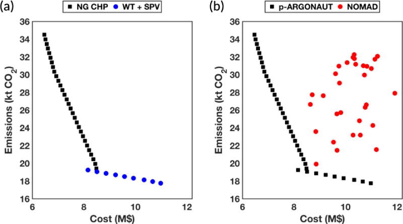
Pareto-frontier for the energy systems design problem in a supermarket obtained using p-ARGONAUT. (a) Pareto-frontier showing the cost-effective design using natural gas-powered CHP technology (NG CHP) with squares and the environmentally friendly design using wind turbine (WT) and solar photovoltaics (SPV) in circles; (b) Comparison of results using p-ARGONAUT, shown in squares, and the NOMAD algorithm, shown in circles.
One of the most important characteristics of the curve shown in Fig. 11(a) is that, each point represents an equally optimal design with different economic and environmental behaviors when different technologies are used as the on-site energy generation technology in a supermarket. For example, the most cost-efficient design is achieved using natural gas-powered CHP system, shown as the very first point on the Pareto-frontier. However, this design completely neglects any constraints on the greenhouse gas emissions and possible impacts on the environment. As a result, CO2 emissions are at its highest level when the cost is minimal. On the contrary, using wind turbine and solar PV provides an environmentally friendly alternative to the natural-gas powered CHP as an on-site energy generation technology in a supermarket. However, the cost of having this system on a supermarket is now at its maximum value, which is $11M.
We have also studied this problem using the ISRES and the NOMAD algorithms, in which the results of this study are summarized in Fig. 11(b). The complete Pareto-curve generated by p-ARGONAUT is now presented in squares whereas the results for the NOMAD algorithm are represented in circles, as shown in Fig. 11(b). It is important to note that the ISRES algorithm is unable to locate any feasible solutions within the maximum allowable number of samples (sample tolerance set to 3000) for this case study over the course of 10 runs for each Pareto-point. As a result, we have only reported the values obtained using the NOMAD algorithm in comparison to the results obtained using p-ARGONAUT. Fig. 11(b) demonstrates that the NOMAD algorithm can locate feasible solutions to the problem in the objective space. However, due to its local exploration strategy, the algorithm struggles to converge to the global optimum at each Pareto-point and can only return local feasible solutions. In addition, a fraction of the NOMAD runs is terminated with high infeasibility, where the algorithm is unable to satisfy all the constraints posed in the problem. On the contrary, p-ARGONAUT is able to report consistent feasible solutions for all the points that construct the Pareto-frontier reported in Fig. 11(a) and (b).
Furthermore, Fig. 12 summarizes the computational performance of the two methods with respect to the elapsed computational time and number of samples collected by each method. Fig. 12(a) and (b) show the elapsed time utilized by each solver for the case with natural gas-powered CHP and for the case with wind turbine and solar PV, respectively. For the natural gas-powered CHP case, we see that both derivative-free solvers perform comparably with each other. However, Fig. 12(c) shows that for the same case study NOMAD collects 5000 points on average per Pareto-point to converge to a feasible solution whereas p-ARGONAUT collects less than 700 samples per Pareto-point. Compared to the results summarized in Fig. 9, p-ARGONAUT converges to the global optimal solution with higher number of samples at every Pareto-point. This is an expected result given that all the derivative-free solvers experience an increase in sampling requirements with increasing problem complexity. This trend is also reflected in NOMAD’s results where there is a gradual increase in the total number of samples collected in each problem set, as shown in Fig. 9 and Fig. 12.
Fig. 12.
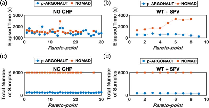
Comparison of computational performance of p-ARGONAUT and NOMAD; (a) Average elapsed time for the p-ARGONAUT and NOMAD algorithms per Pareto-point in natural gas-powered CHP (NG CHP) case; (b) Average elapsed time for the p-ARGONAUT and NOMAD algorithms per Pareto-point in wind turbine and solar PV (WT + SPV) case; (c) Average total number of samples collected by the p-ARGONAUT and NOMAD algorithms per Pareto-point in NG CHP case; (d) Average total number of samples collected by the p-ARGONAUT and NOMAD algorithms per Pareto-point in WT + SPV case. Circles represent the results for p-ARGONAUT whereas the squares represent the results for NOMAD.
Moreover, for the case with wind turbine and solar PV, we observe that p-ARGONAUT collects significantly low number of samples to converge to global optimum, as shown in Fig. 12(d). It is important to note that for both cases NOMAD consistently hits the maximum number of allowable samples and returns the best-found solution from these 5000 collected points. Furthermore, like in Fig. 11, the results with infeasible solutions are not plotted in Fig. 12. As a result, we can clearly see that for certain sub-problems in both natural gas-powered CHP and wind turbine and solar PV cases, NOMAD is unable to locate feasible solutions over 10 repetitive runs. Thus, it is safe to say that p-ARGONAUT outperforms other available derivative-free software, both in terms of computational performance and in accuracy for locating the global solution for the MOO of energy market design problem.
We have repeated the same case study with the updated values for the prices and efficiencies where the values of these new parameters are summarized in Tables 7 and 8. The results for the energy market design problem with the updated parameters are summarized in Fig. 13.
Fig. 13.
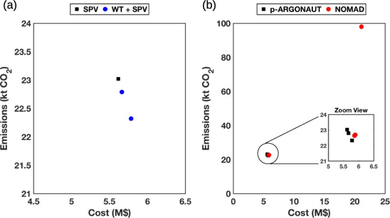
Multi-objective optimization results using the updated parameters; (a) Pareto-frontier obtained using p-ARGONAUT where the cost-effective design is achieved via solar photovoltaics (SPV), shown in squares, and the environmentally friendly design is achieved using wind turbine (WT) and solar photovoltaics (WT + SPV), shown in circles; (b) comparison of results using p-ARGONAUT, shown in squares, and the NOMAD algorithm, shown in circles.
Interestingly, Fig. 13(a) shows that the most economic on-site energy generation for a supermarket is achieved via solar PV rather than the natural-gas powered CHP. With the recent developments in the solar PV technology, we see that the solar PV’s are more available throughout the year with lower operating costs and higher capacities. As a result, the technology selection has shifted from natural gas-based to a renewable-based system for the supermarket. Thus, it is possible to minimize both the cost and the CO2 emissions of on-site energy generation using solar PV, which also replaces the existing trade-off between the two objectives for this system, while shrinking the Pareto-curve into a single optimum. In addition, Fig. 13(a) shows that using wind turbine and solar PV together as the on-site energy generation technologies result in lower CO2 emissions. Yet again, as in Fig. 11, as the CO2 emissions decrease, the cost of having that technology increases. Moreover, Fig. 13(b) shows the comparison between the results obtained using p-ARGONAUT and the NOMAD algorithm. Like in the previous results, ISRES runs are terminated with high infeasibility for all three points constructing the Pareto-frontier hence, not included in the plots. The results show that NOMAD can locate local feasible solutions but it struggles to find the Pareto-optimal solution for the current values of the energy market design problem where a fraction of runs has ended with high infeasibility. Especially for one of the points of the Pareto-curve, we observe that the NOMAD solution is quite distant from the Pareto-optimal solution designated by p-ARGONAUT. Fig. 13(b) also shows a zoomed view of the results that are close to each other. The zoomed picture shows that the NOMAD solutions are very close to the optimal solutions found by p-ARGONAUT but still does not perfectly capture the global solution.
6. Conclusions
In this work, we have implemented a data-driven hybrid methodology that integrates surrogate model identification and deterministic global optimization through the parallel AlgoRithms for Global Optimization of coNstrAined grey-box compUTational problems (p-ARGONAUT) algorithm for the global optimization of general constrained grey-box multi-objective optimization (MOO) problems. We have tested our parallel framework, which is designed to solve high-dimensional general constrained grey-box problems via utilizing high-performance computing on several stages of the algorithm, on three constrained MOO benchmark problems and a detailed case study of an energy market design problem for a commercial building. In each case study, we have implemented the well-known ε-constraint method to convert the MOO problem into series of single-objective optimization sub-problems and used p-ARGONAUT to globally optimize the resulting constrained grey-box problems. The results show that p-ARGONAUT can consistently and efficiently identify the Pareto-frontier, which entails all the trade-off solutions that are equally optimal with respect to each other, under varying conditions and dimensions of constrained grey-box multi-objective problems. Furthermore, p-ARGONAUT outperforms other available derivative-free algorithms by providing consistent feasible solutions for the energy systems design case study, involving numerous equality constraints which is typically challenging for general derivative-free algorithms.
Highlights.
p-ARGONAUT is extended towards constrained multi-objective optimization problems.
Data-driven approach is followed to optimize an energy market design problem.
The accuracy and consistency of the method is evaluated under equality constraints.
Computational results are compared with a number of available software.
Acknowledgments
The authors would like to dedicate this work to Professor Christodoulos A. Floudas whose guidance, mentorship and leadership will truly be missed. Authors would like to acknowledge the support provided by the Texas A&M Energy Institute, National Science Foundation (NSF CBET-1548540), U.S. National Institute of Health Superfund Research Program (NIH P42-ES027704), and the Texas A&M University Superfund Research Center. The manuscript contents are solely the responsibility of the grantee and do not necessarily represent the official views of the NIH. Further, the NIH does not endorse the purchase of any commercial products or services mentioned in the publication.
Footnotes
Publisher's Disclaimer: This is a PDF file of an unedited manuscript that has been accepted for publication. As a service to our customers we are providing this early version of the manuscript. The manuscript will undergo copyediting, typesetting, and review of the resulting proof before it is published in its final citable form. Please note that during the production process errors may be discovered which could affect the content, and all legal disclaimers that apply to the journal pertain.
References
- Abdelkafi O, Idoumghar L, Lepagnot J, Paillaud JL, Deroche I, Baumes L, Collet P. Using a novel parallel genetic hybrid algorithm to generate and determine new zeolite frameworks. Comput Chem Eng. 2017;98:50–60. [Google Scholar]
- Abramson MA, Audet C, Couture G, Dennis JE, Jr, Le Digabel S, Tribes C. The NOMAD project. 2015 https://www.gerad.ca/nomad/ (accessed 16 January 2018)
- BASIS. Report on conversion efficiency of biomass. 2015 http://www.basisbioenergy.eu/fileadmin/BASIS/D3.5_Report_on_conversion_efficiency_of_biomass.pdf.
- Beykal B, Boukouvala F, Floudas CA, Sorek N, Zalavadia H, Gildin E. Global optimization of grey-box computational systems using surrogate functions and application to highly constrained oil-field operations. Comput Chem Eng. 2018 doi: 10.1016/j.compchemeng.2018.02.017. https://doi.org/10.1016/j.compchemeng.2018.01.005 [DOI] [PMC free article] [PubMed]
- Bhattacharjee KS, Singh HK, Ray T. Multi-Objective Optimization With Multiple Spatially Distributed Surrogates. J Mech Design. 2016;138:91401–91410. [Google Scholar]
- Boukouvala F, Floudas CA. ARGONAUT: AlgoRithms for Global Optimization of coNstrAined grey-box compUTational problems. Optim Lett. 2017;11:895–913. [Google Scholar]
- Boukouvala F, Hasan MMF, Floudas CA. Global optimization of general constrained grey-box models: new method and its application to constrained PDEs for pressure swing adsorption. J Glob Optim. 2017;67:3–42. [Google Scholar]
- Boukouvala F, Misener R, Floudas CA. Global optimization advances in mixed-integer nonlinear programming, MINLP, and constrained derivative-free optimization, CDFO. Eur J Oper Res. 2016;252:701–727. [Google Scholar]
- Chafekar D, Xuan J, Rasheed K. Constrained Multi-objective Optimization Using Steady State Genetic Algorithms. In: Cantú-Paz E, et al., editors. Genetic and Evolutionary Computation — GECCO 2003: Genetic and Evolutionary Computation Conference Chicago, IL, USA, July 12–16, 2003 Proceedings, Part I. Springer Berlin Heidelberg; Berlin, Heidelberg: 2003. pp. 813–824. [Google Scholar]
- Clark PA, Westerberg AW. Optimization for design problems having more than one objective. Comput Chem Eng. 1983;7:259–278. [Google Scholar]
- Coello CC, Lamont GB, Veldhuizen DAv. Evolutionary Algorithms for Solving Multi-Objective Problems. second. Springer; New York: 2007. [Google Scholar]
- Datta R, Regis RG. A surrogate-assisted evolution strategy for constrained multi-objective optimization. Expert Syst Appl. 2016;57:270–284. [Google Scholar]
- di Pierro F, Khu ST, Savić D, Berardi L. Efficient multi-objective optimal design of water distribution networks on a budget of simulations using hybrid algorithms. Environ Modell Softw. 2009;24:202–213. [Google Scholar]
- Drud A. CONOPT—a large-scale GRG code. ORSA J Comput. 1994;6:207–216. [Google Scholar]
- EIA. State electricity profiles. 2016a https://www.eia.gov/electricity/state/unitedstates/ (accessed 06.11.2017)
- EIA. Updated buildings sector appliance and equipment costs and efficiencies. 2016b https://www.eia.gov/analysis/studies/buildings/equipcosts/pdf/full.pdf.
- EIA. Monthly densified biomass fuel report. 2017a https://www.eia.gov/biofuels/biomass/ (accessed 06.11.2017)
- EIA. (Document Number: DOE/EIA-0035(2017/5)).Monthly energy review, May 2017. 2017b https://www.eia.gov/totalenergy/data/monthly/
- EPA. Biomass combined heat and power catalog of technologies. 2007 https://www.epa.gov/sites/production/files/2015-07/documents/biomass_combined_heat_and_power_catalog_of_technologies_v.1.1.pdf.
- EPA. Emission factors for greenhouse gas inventories. 2015 https://www.epa.gov/sites/production/files/2016-09/documents/emission-factors_nov_2015_v2.pdf (accessed 06.11.2017)
- Fan Z, Liu J, Sorensen T, Wang P. Improved differential evolution based on stochastic ranking for robust layout synthesis of MEMS components. IEEE Trans Ind Electron. 2009;56:937–948. [Google Scholar]
- Feliot P, Bect J, Vazquez E. A Bayesian approach to constrained single- and multi-objective optimization. J Glob Optim. 2017;67:97–133. [Google Scholar]
- Floudas CA, Niziolek AM, Onel O, Matthews LR. Multi-scale systems engineering for energy and the environment: challenges and opportunities. AIChE J. 2016;62:602–623. [Google Scholar]
- Gong D-w, Zhang Y, Qi C-l. Environmental/economic power dispatch using a hybrid multi-objective optimization algorithm. Int J Elec Power. 2010;32:607–614. [Google Scholar]
- Jain H, Deb K. An Evolutionary Many-Objective Optimization Algorithm Using Reference-Point Based Nondominated Sorting Approach, Part II: Handling Constraints and Extending to an Adaptive Approach. IEEE Trans Evol Comput. 2014;18:602–622. [Google Scholar]
- Johnson SG. The NLopt nonlinear-optimization package. 2014 http://ab-initio.mit.edu/nlopt (accessed 16 January 2018)
- Le Digabel S. Algorithm 909: NOMAD: nonlinear optimization with the MADS algorithm. ACM Trans Math Softw. 2011;37:1–15. [Google Scholar]
- Liu P, Pistikopoulos EN, Li Z. An energy systems engineering approach to the optimal design of energy systems in commercial buildings. Energ Policy. 2010;38:4224–4231. [Google Scholar]
- Martínez-Frutos J, Herrero-Pérez D. Kriging-based infill sampling criterion for constraint handling in multi-objective optimization. J Glob Optim. 2016;64:97–115. [Google Scholar]
- Miettinen K. Nonlinear Multiobjective Optimization. Springer; New York: 1998. [Google Scholar]
- Misener R, Floudas CA. Global optimization of mixed-integer models with quadratic and signomial functions: a review. Appl Comput Math. 2012;11:317–336. [Google Scholar]
- Misener R, Floudas CA. GloMIQO: Global mixed-integer quadratic optimizer. J Glob Optim. 2013;57:3–50. [Google Scholar]
- Misener R, Floudas CA. ANTIGONE: Algorithms for coNTinuous/Integer Global Optimization of Nonlinear Equations. J Glob Optim. 2014;59:503–526. [Google Scholar]
- NREL. Energy analysis: distributed generation renewable energy estimate of costs. 2016 http://www.nrel.gov/analysis/tech_lcoe_re_cost_est.html.
- Rangaiah GP, Bonilla-Petriciolet A. Multi-Objective Optimization in Chemical Engineering: Developments and Applications. John Wiley & Sons, Ltd; United Kingdom: 2013. [Google Scholar]
- Ray T, Tai K, Seow KC. Multiobjective design optimization by an evolutionary algorithm. Eng Optimiz. 2001;33:399–424. [Google Scholar]
- Regis RG. Multi-objective constrained black-box optimization using radial basis function surrogates. J Comput Sci. 2016;16:140–155. [Google Scholar]
- Runarsson TP, Yao X. Search biases in constrained evolutionary optimization. IEEE T Syst Man Cy C. 2005;35:233–243. [Google Scholar]
- Sanchis J, Martínez MA, Blasco X. Integrated multiobjective optimization and a priori preferences using genetic algorithms. Inform Sciences. 2008;178:931–951. [Google Scholar]
- Singh P, Couckuyt I, Ferranti F, Dhaene T. IEEE Congress on Evolutionary Computation. Beijing: IEEE; 2014. A constrained multi-objective surrogate-based optimization algorithm. [Google Scholar]
- Sorek N, Gildin E, Boukouvala F, Beykal B, Floudas CA. Dimensionality reduction for production optimization using polynomial approximations. Comput Geosci. 2017;21:247–266. [Google Scholar]
- Tabatabaei M, Hakanen J, Hartikainen M, Miettinen K, Sindhya K. A survey on handling computationally expensive multiobjective optimization problems using surrogates: non-nature inspired methods. Struct Multidisc Optim. 2015;52:1–25. [Google Scholar]
- Toffolo A, Lazzaretto A. Evolutionary algorithms for multi-objective energetic and economic optimization in thermal system design. Energy. 2002;27:549–567. [Google Scholar]
- Wang L, Singh C. Environmental/economic power dispatch using a fuzzified multi-objective particle swarm optimization algorithm. Electr Pow Syst Res. 2007;77:1654–1664. [Google Scholar]
- Zielinski K, Peters D, Laur R. Third International Conference on Computational Intelligence, Robotics and Autonomous Systems. Singapore: CIRAS; 2005. Constrained multi-objective optimization using differential evolution. [Google Scholar]