Whole-Brain Calcium Imaging during Physiological Vestibular Stimulation in Larval Zebrafish

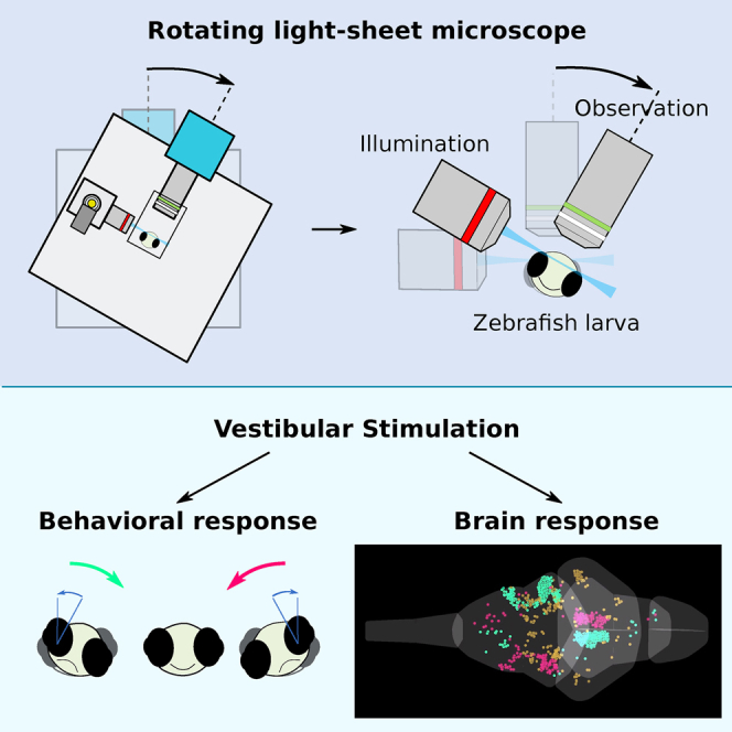
Summary

The vestibular apparatus provides animals with postural and movement-related information that is essential to adequately execute numerous sensorimotor tasks. In order to activate this sensory system in a physiological manner, one needs to macroscopically rotate or translate the animal’s head, which in turn renders simultaneous neural recordings highly challenging. Here we report on a novel miniaturized, light-sheet microscope that can be dynamically co-rotated with a head-restrained zebrafish larva, enabling controlled vestibular stimulation. The mechanical rigidity of the microscope allows one to perform whole-brain functional imaging with state-of-the-art resolution and signal-to-noise ratio while imposing up to 25° in angular position and 6,000°/s² in rotational acceleration. We illustrate the potential of this novel setup by producing the first whole-brain response maps to sinusoidal and stepwise vestibular stimulation. The responsive population spans multiple brain areas and displays bilateral symmetry, and its organization is highly stereotypic across individuals. Using Fourier and regression analysis, we identified three major functional clusters that exhibit well-defined phasic and tonic response patterns to vestibular stimulation. Our rotatable light-sheet microscope provides a unique tool for systematically studying vestibular processing in the vertebrate brain and extends the potential of virtual-reality systems to explore complex multisensory and motor integration during simulated 3D navigation.

Graphical Abstract

Highlights

• •A novel miniaturized rotatable light-sheet microscope is reported
• •It allows brain-wide calcium imaging during vestibular stimulation in zebrafish larvae
• •The whole-brain neuronal response to sinusoidal and stepwise vestibular stimulation is mapped
• •Neurons were clustered according to their tonic and phasic response profiles

Migault et al. developed a novel miniaturized ultra-stable light-sheet microscope to perform functional imaging during dynamic vestibular stimulation of a tethered zebrafish. The whole-brain response to sinusoidal and stepwise vestibular stimulation is mapped and characterized by Fourier and regression analysis.

Introduction

Functional imaging is a powerful alternative to electrophysiology for monitoring brain activity in vivo. When performed on small and transparent animals such as zebrafish larvae, it allows long-term, non-invasive recording of the entire brain, enabling large-scale analysis of neuronal circuits [1, 2, 3, 4, 5, 6]. This method can be combined with various sensory stimulations—such as visual, auditory, thermal, or olfactory—and behavioral monitoring in order to probe the neural computations underlying complex sensorimotor tasks [4, 7, 8, 9, 10, 11, 12].

When zebrafish navigate through their 3D environment, their vestibular apparatus continuously informs the brain about the body orientation relative to gravity as well as its translational and rotational accelerations. Vestibular information is involved in locomotion initiation [13], postural control, and gaze stabilization [14, 15]. Vestibular cues also enable larval zebrafish to find the water surface, in order to inflate their swim bladder, or to navigate to the ground when stressed. Vestibular deficient animals are not viable [16]. In spite of its crucial role, the vestibular system remains a sensory modality whose neural substrate cannot be probed with brain-scale functional imaging. This owes to the particular challenge posed by this sensory system, whose physiological activation requires dynamically rotating and/or translating the animal. If performed under a non-moving microscope, such movements would constantly change the imaged brain section, precluding the possibility of monitoring the activity of individual neurons over time.

Favre-Bulle et al. showed that vestibular behavioral responses can be evoked in head-fixed larvae by directly moving utricular otoliths, the small structures in the organs of the inner ears that convey vestibular information, using optical tweezers [17]. This fictive stimulation approach offers large flexibility in terms of achievable stimulus patterns and is shown, in a study reported alongside this paper, to be compatible with functional imaging [18]. However, because the force exerted by the optical tweezers on the otolith is not calibrated, this method does not allow delivering natural-like vestibular stimuli in a controlled and reproducible way. A complementary avenue may also be provided by functional recording in freely swimming fish, as was recently proposed [19, 20, 21]. However, it lacks the possibility of disentangling vestibular from motor variables and is restricted to 2D trajectories. Here we report on the development and application of a rotating light-sheet microscope that co-rotates the head-tethered animal, thus stimulating the vestibular system while providing stable imaging conditions. This compact rotating microscope offers single-cell-resolved whole-brain recordings during physiological dynamic vestibular stimulation in larval zebrafish.

We first detail the design of the rotating microscope and its characterization in terms of mechanical stability and imaging performances. Next, we demonstrate the system’s full potential by simultaneously monitoring brain-scale neuronal activity and compensatory eye movements in zebrafish larvae submitted to sinusoidal and stepwise rolling movements. In the second part, we focus on the neuronal response using either paralyzed or bi-enucleated fish in order to minimize or suppress visual inputs associated with compensatory eye movements. We quantitatively characterized the brain-wide vestibular response. The response map was found to encompass extended neuronal assembly spanning multiple brain areas and exhibiting highly stereotypic bilateral symmetry. Using Fourier and multi-linear regression analysis, we classified these neuronal populations based on their phase relation with respect to sinusoidal stimulation and according to their respective phasic and tonic responses to stepwise stimuli. In addition to the technical developments reported here, we provide an open-source graphical tool, called the “Fishualizer,” to visualize, inspect, and analyze 4D functional imaging data.

Results

A Miniaturized Rotating Digital-Scanning Light-Sheet Microscope

Delivering physiological vestibular stimulation in combination with functional imaging requires dynamically co-rotating the entire imaging system and the animal (Figure 1A), which in turn imposes stringent demands on its mechanical rigidity. Any mechanical distortion resulting from the changing gravitational forces during microscope rotation may indeed displace the imaging plane. Such displacements would transiently bring another set of neurons into focus, leading to detrimental artifacts in the fluorescence recordings. In order to mitigate these issues, we designed a miniaturized illumination unit for 3D, digitally scanned light-sheet microscopy. By reducing the number of optical components to a minimum, we obtained a ten-fold reduction in size of the optical path as compared to standard, digitally scanned light-sheet microscopes. This compact design eliminates most mechanical distortions and makes the microscope largely insensitive to vibrations.

Figure 1.

Experimental Setup and Imaging Performance

(A) Schematic of the rotating microscope setup with the light-sheet unit (LU), mounted zebrafish (ZF), and detection unit (DU). The close-up image illustrates how the fish rotates together with the microscope such that the light sheet and the detection focal plane coincide for any rotation angle. Stimulation angles are counted as positive in the direction indicated by the arrow. The fish faces the breadboard with its long body axis aligned with the microscope rotation axis.

(B) Schematic of the light-sheet-forming unit. Inset: measured light-sheet profile (black) and adjusted with the theoretical Gaussian beam profile (red).

(C) Details of the light-sheet unit. The left part illustrates in a top view the scanning mechanism for the light-sheet formation. The right part illustrates in a side view the ray diagram for the z scanning of the light sheet. The scanning mirror is omitted for clarity. The green ellipse schematizes the fluorescent zebrafish brain. The photographs of the light-sheet unit corresponding to top and side views are shown below the two schemes. The two metallic disks allow rotating the unit for alignment.

(D) Sagittal and coronal sections of a volumetric whole-brain scan of a 6-day-old zebrafish larva with pan-neuronal GCaMP6s expression (Tg(elavl3:H2B-GCaMP6s)). The four insets show quasi-single-cell resolution and the result of the automatic segmentation process. Scale bars, 50 μm (main image) and 25 μm (insets).

See also Video S1.

The light sheet is produced by imaging the output of an optical fiber into the sample using two objectives with low numerical aperture (NA) and a scanning mirror (Figure 1B). In this design, we omitted a relay system that is conventionally used to ensure parallel beam deflection by bringing the pivoting point of the mirror onto the back focal plane of the illumination objective. However, we calculated that the resulting laser-pointing variation across the approximately square-millimeter field of view is less than α = 0.4° (Figure 1C; STAR Methods). Because it occurs within the light-sheet plane, this deviation has no impact on the imaging performance. The divergence of the beam at the fiber outlet offers an adequate numerical aperture for obtaining a micron-thick light sheet without the need to introduce a beam-expander system. Notably, this configuration compensates for spherical aberrations, as the laser passes through the two identical objectives in reverse direction. Z scanning (Figures 1B and 1C; Video S1) is obtained by directly moving the fiber outlet using a piezo crystal. This is possible because the telescope formed by the two objectives conjugates the light-sheet waist to the fiber outlet. Although the presence of the scanning mirror between the two objectives abolishes perfect telecentricity, the resulting pointing error α is less than 0.4° (Figure 1C; STAR Methods) for the scan range of 250 μm and corresponds to a displacement of the light sheet relative to the focal plane of less than 3% of the light-sheet thickness, corresponding to a maximal displacement at the most lateral side of the sample of less than 2 μm.

Video S1. High-Resolution Volumetric Brain Scan, Related to Figure 1

6dpf old larval zebrafish with pan-neuronal nuclear-localized GCaMP6s expression, 1 μm inter-section separation.

With this compact design, the light-sheet unit dimensions are only 9 × 6 × 10 cm (Figures 1B and 1C) and the light sheet can be aligned in a straightforward way by rotating and translating the entire unit. All optical elements—including the fluorescence detection system, a behavior tracking module, and the sample holder—are mounted onto a breadboard (Figure 1A), attached on an ultra-stable high-load rotation stage (ALAR150SP; Aerotech), which can accelerate the microscope to an angular velocity of 60°/s in less than 10 ms with minimal backlash. The light-sheet profile is consistent with the predictions of Gaussian optics with a half-width at 1/e² of 2.04 ± 0.02 μm (mean ± SD) (Figure 1B, inset; STAR Methods). This miniaturized design provides optical sectioning similar to state-of-the-art, digital-scanning light-sheet microscopes, and thus offers quasi-single-cell resolution throughout the brain, with the exception of the most ventral regions between the eyes, which are shadowed. The image resolution is sufficient for automatic cellular segmentation in most parts of the brain [1]. To demonstrate the optical quality of the system, a high-resolution volumetric brain scan of a 6-dpf (days post-fertilization) larval zebrafish brain is provided (Figure 1D; Video S1; with GCaMP6s expressed pan-neuronally and confined to the nuclei).

Imaging Conditions Remain Stable during Microscope Rotation

We characterized the stability of our setup upon rotation using 3D tracking of microspheres. In brief (for details, see STAR Methods), the image of fluorescent microspheres 1 μm in diameter embedded in agarose shows a characteristic interference pattern in the form of concentric rings. Their diameter is a function of the microsphere position relative to the focal plane (Figures 2A and 2B). Sample movements can thus be characterized in 3D by monitoring the rings’ center positions and radii over time. The tracking accuracy in the z direction is 10 nm (SD, N = 5), as deduced from calibration measurements (Figure 2C). We found that during sinusoidal microscope rotation over ±20°, the scan volume moves by less than 500 nm in the z direction, i.e., only ∼6% of the typical soma diameter (∼8 μm), and by less than 2 μm in the x-y plane (Figure 2D).

Figure 2.

Stability Characterization and Noise-Level Estimation

(A) Characteristic interference pattern of a fluorescent microsphere displaced relative to the focal plane of the detection objective.

(B) Radial intensity profile averaged over all angles as a function of the imposed objective height. This profile serves as a look-up table (LUT) to quantify z movements of the microsphere during microscope rotation. The dashed line indicates the fit position for the profile shown in (A).

(C) Performance test of the z tracking algorithm. A control signal drives a piezo to displace the detection objective in steps of 0.5 μm (red), and the relative distance of the microsphere to the objective (blue; error bars indicate SD; N = 5) is computed by fitting the instantaneous intensity profile of the microsphere onto the LUT shown in (B).

(D) Characterization of the shift along the z direction of the scanned volume as a function of the microscope rotation angle (blue; error bars indicate SD, N = 5). Rotation direction is from −20° to +20° in blue and the reverse rotation is in red. The inset shows the corresponding movements in the x-y plane. The schematic defines the coordinate system.

(E) Step stimulation protocol used for estimating the mechanically induced noise level.

(F) Distribution of the intensity change per pixel induced by a −15° microscope rotation relative to the intensity value measured just before the step (RFP- [red] and GCaMP6s- [blue] expressing fish). Light colors correspond to the intrinsic noise distribution measured in the absence of microscope rotation. Data were centered and normalized via Gaussian fits.

(G) Mean mechanically induced noise level (Δσ) measured with RFP- (red) and GCaMP6s- (blue) expressing fish as a function of microscope angle (error bars indicate SD; N = 3 fish).

The in-plane displacements can be corrected during post-processing using successive image cross-correlation. In contrast, the axial drift cannot be compensated, and may introduce small artifactual modulations of the fluorescence signals. To quantify the noise level associated with these movements, we performed control experiments with paralyzed fish pan-neuronally expressing a red fluorescent protein (HuC:RFP), which does not report neuronal activity. We measured the distributions of the intensity change per pixel induced by stepwise microsocpe rotation of various amplitudes and compared them to the intrinsic noise distribution when the microsocpe is static at zero degree (Figure 2E; Figure 2F, light and dark red). The difference of the SDs of these two distributions (Δσ) is used as a measure of the mechanically induced fluorescence noise. We found that Δσ increases with the rotation amplitude but remains below 2% in ΔF/F (averaged over three fish) over a range of ±25° (Figure 2G, red). We then repeated the same analysis with paralyzed fish expressing the calcium reporter GCaMP6s pan-neuronally (Figure 2F, light and dark blue; Figure 2G, blue). In these experiments, Δσ remains below 3% ΔF/F (averaged over three fish) and shows the same dependence with the rotation angles as measured with the RFP fish. Even during rotation of the microscope, the imaging quality of the miniaturized setup thus remains equivalent to state-of-the-art light-sheet setups [1] with respect to signal-to-noise ratio and spatial resolution.

Combined Whole-Brain Imaging and Behavioral Monitoring during Dynamic Vestibular Stimulation

To demonstrate the full potential of our platform, we simultaneously monitored brain-wide neuronal activity and the evoked behavioral response during sinusoidal and stepwise rotation (for stimulation and acquisition details, see STAR Methods). For these experiments, larvae expressing GCaMP6s pan-neuronally were partially embedded in agarose to allow free eye movements (Figure S1). The fish responded to rolling stimulation via the gravito-inertial, vestibulo-ocular reflex (maculo-ocular reflex) with compensatory eye movements to maintain clear vision (Figure 3A). Both stimulation protocols evoked extended activation of neuronal activity across the larval brain. The neuronal activity appeared correlated to the stimulus, localized to specific brain regions, and antisymmetric with respect to the mid-sagittal plane, as shown in Video S2 (part I: sinusoidal stimulation; part II: step stimulation). Example activity traces of selected regions are shown in Figure 3C. The activity of individual neurons followed the sinusoidal stimulus over time with various well-defined phase shifts relative to the microscope rotation (Figure 3C, left). During stepwise stimulation, we observed, among others, tonic-like responses tuned to the leftward or rightward angular position of the fish. These experiments demonstrate that the developed platform provides the necessary stability and imaging resolution to monitor brain-scale neuronal activity alongside behavioral responses evoked by natural vestibular stimulation.

Figure 3.

Behavioral and Neuronal Response to Sinusoidal and Stepwise Dynamic Vestibular Stimulation

(A) Top: schematic illustrating the rolling rotation of the fish when the microscope rotates and the evoked compensatory eye movements. Angles are counted as positive in the clockwise direction, i.e., when the fish rolls toward its right side. Bottom: trial-averaged behavioral response to sinusoidal and to step stimulation (dashed black) and associated compensatory eye movements (green). The sign of the eye orientation has been reversed to facilitate comparison.

(B) Three views showing the location of the regions of interest (red, blue, and gray disks) in Z-Brain coordinates from which the fluorescence example time traces shown in (C) were extracted. The outline of the optic tectum (OT) and the trochlear nucleus (nIV) are shown.

(C) Example fluorescence traces (raw signals and trial average). Horizontal dashed lines indicate zero, which is defined by the calculated fluorescence baseline (see STAR Methods). Left: responses to sinusoidal stimulation (blue and gray disks from rostral to caudal in B). Right: responses to step stimulation (red-numbered disks). OT, optic tectrum; nIV, trochlear nucleus; VS, vestibulo-spinal neurons; Rh, rhombomere. All data were recorded with Tg(elavl3:GCaMP6s) fish.

See also Video S2.

Video S2. Functional Brain-wide Response to Sinusoidal and Stepwise Vestibular Rolling Stimulation (GCaMP6s Localized to Cytoplasm), Related to Figure 3

Top: Shown are 4 out of 20 recorded brain sections. Bottom left: The rotating microscope. Bottom right: Front view of the zebrafish larva performing compensatory eye movements in response to the vestibular rolling stimulus. PART I: Average over 120 cycles of sinusoidal stimulation (2x accelerated). From this recording we extracted the data shown in Figure 3C. Stimulation parameters: 0.2 Hz stimulation frequency, ± 10° stimulation amplitude. Acquisition parameters: 2.5 stacks per second, 20 brain sections, 10 μm inter-slice separation. PART II: Average over 10 step stimulation cycles (12x accelerated). From this recording we extracted the data shown in Figure 3D. Stimulation parameters: 30°/s maximal angular velocity, 3 steps per cycle with 10°, 15° and 20° amplitude, 10 s dwell time. Acquisition parameters: 2.5 stacks per second, 20 brain sections, 10 μm inter-slice separation.

In both sets of experiments, we noticed stimulus-correlated activity in the tectum and in the tectal neuropil (Video S2; first example trace in Figure 3C), two regions that are known to be major retino-recipient areas. We suspected that this activity might be partly or entirely evoked by concurrent stimulation of the visual sensory system induced by the eyes’ rotation. Although the experiments were conducted in the dark, the blue laser inevitably produces a diffuse illumination of the specimen chamber, thus providing visual cues to the animal. Because the chamber is static with respect to the animal body (head-attached object), this residual visual pattern is expected to stabilize the eye position, thus conflicting with the vestibulo-driven compensatory eye rotation. However, this visually driven counteracting force is likely to be small, as the gain of the behavioral response (the ratio between eyes and body rotation) was measured to be 0.61 ± 0.2 (SD, N = 9), i.e., even larger than the values reported in behavioral assays performed in complete darkness [14]. Hence, if visual inputs are present, their impact on eye dynamics is certainly modest in comparison with the vestibular inputs. However, this does not rule out the possibility that the visual stimulation may account for some of the responses observed in visual responsive regions. In order to minimize any non-vestibular inputs, all experiments reported in the following were carried out with paralyzed and fully embedded fish, thus excluding (1) visual inputs associated with retinal slip evoked by eye movements, (2) proprioceptive sensory inputs induced by muscle contraction, and (3) hydromechanical inputs from the lateral line. As a further control, we replicated all experiments with bi-enucleated fish.

Neuronal Responses to Dynamic Vestibular Stimulation Are Left-Right Symmetric and Highly Stereotypic

Sinusoidal rolling stimulation (0.2-Hz frequency and ±10° amplitude) were delivered to paralyzed fish fully embedded in agarose (nuclear elavl3:H2B-GCaMP6s). We observed intense brain-wide neuronal activity, as shown in Video S3. We quantified this brain-wide vestibular response by computing via Fourier analysis the amplitude (in units of signal to noise) and the phase shift of the signal relative to the stimulus (STAR Methods) for every brain voxel (0.8 × 0.8 × 10 μm). We found a continuum of phase shifts in the response, but the largest response amplitude was found predominantly for phase shifts of either 7/8π or 15/8π (Figure 4A, top). Notice that these phase shifts were directly computed from the fluorescence signals, and thus need to be offset by Δφ_GCaMP = −1.35 rad to account for the calcium reporter delayed response in order to capture the actual spike rate dynamics (see STAR Methods). Taking into account this correction, these two predominant populations appear to display a maximum response for intermediate values of the rotational angle and velocity, i.e., when either both are positive (7/8π − Δφ_GCaMP) or negative (15/8π − Δφ_GCaMP) (Figure 4A, bottom, magenta and pale green arrows, respectively). These neurons can thus be described as mixed angle-and-velocity tuned.

Figure 4.

Phase Maps of Functional Brain-wide Response to Sinusoidal Vestibular Rolling Stimulation, Paralyzed Fish

(A) Top: polar plot of the fluorescence response amplitude per neuron measured in units of signal to noise (STAR Methods) and plotted against the phase delay of the response relative to the stimulus. The color code indicates the phase shift. The dashed line indicates the expected position of a zero-phase-shift neuronal signal once corrected for the phase delay introduced by the GCaMP6s sensor (STAR Methods). Bottom: schematic showing one stimulus cycle (black dashed). Arrows indicate the phase in the cycle where the neurons with the dominant response (black line, top) have their maximal response when taking into account the delay introduced by the GCaMP6s sensor.

(B) Top: ten selected phase map layers of an example fish after registration on the Z-Brain reference brain. The delineated brain areas are from the Z-Brain atlas. Bottom: close-up views of regions shown by the dashed rectangles.

(C) Fractions of responding neurons and the corresponding phase-shift distribution in the 13 selected brain areas.

(D) Maximum-projection views of the phase map shown in (B) and separated into the four phase intervals depicted in (A). For each phase interval, a maximum projection from left to the midline and from dorsal to ventral is shown.

(E) Fraction of responding neurons and the corresponding phase distribution for the 13 selected brain areas.

(F) Average phase maps. Left: average of N = 8 paralyzed fish. Right: average of N = 9 bi-enucleated paralyzed fish. Maximum projections from left to the midline and from dorsal to ventral are shown.

C, caudal; D, dorsal; Hab, habenula; IO, inferior olive; L, left; R, right; Ro, rostral; TL, torus longitudinalis; Teg, tegmentum; nMLF, nuclear medial fasciculus; nIII, oculomotor nucleus; nIV, trochlear nucleus; Cer, cerebellum; V, ventral; Rh, rhombomere. All data were recorded in Tg(elavl3:H2B-GCaMP6s) fish. Scale bars, 50 μm and 20 μm (close-up views in B). See also Figures S2–S4 and Videos S3 and S4.

Video S3. Functional Brain-wide Response to Sinusoidal Vestibular Rolling Stimulation (Nuclear-Localized GCaMP6s), Related to Figure 4

Average over 70 stimulation cycles (2x accelerated). Shown are 8 out of 20 recorded sections. Stimulation parameters: 0.2 Hz stimulation frequency, ± 10° stimulation amplitude. Acquisition parameters: 2.5 stacks per second, 20 brain sections, 10 μm inter-slice separation. PART I: paralyzed fish. PART II: bi-enucleated paralyzed fish.

From the pixel-wise phase-shift measurement, we computed a 3D phase map (Figures 4B and 4C; Video S4, part I). This map revealed that neurons displaying similar phase shifts tend to spatially organize into well-defined clusters that are mirror symmetric with respect to the mid-sagittal plane. Figure 4B shows ten selected layers of this example phase map after registration on the Z-Brain atlas [22] (see STAR Methods). We found responding neurons in the torus longitudinalis, habenula, optic tectum, and the tegmentum including the nucleus of the medial longitudinal fasciculus (nMLF), oculomotor nucleus (nIII), and trochlear nucleus (nIV). Large populations of active neurons were also found in the cerebellum and in the hindbrain, in particular in the octavolateral nucleus around the ear (vestibular nucleus), tangential nucleus (white arrows), vestibular spinal neurons (white arrowheads), and inferior olive. Responses in the thalamus, pretectum, and telencephalon are weak and thus hardly distinguishable from spontaneous neuronal activity (which happens to be particularly intense in the telencephalon). In most responsive brain regions the phase map is spatially organized, with a clear separation between the two hemispheres (e.g., in the tegmentum, vestibular spinal neurons, or rhombomere 7). However, we also observed regions with spatially heterogeneous phase responses, e.g., in the habenula, torus longitudinalis, or cerebellum (Figure 4B, bottom). The fraction of highly responsive neurons and the corresponding phase profile for 13 selected brain regions are shown in Figure 4C, revealing a gradual increase of positive phase shifts (i.e., from magenta-green to blue-orange) from rostral to caudal. For this analysis, we recalculated the phase map per neuron after cellular segmentation (see STAR Methods).

Video S4. Animated Multi-angle View of the Z-Projection of the Mean Phase Map (Paralyzed Fish with Eyes; Nuclear-Localized GCaMP6s), Related to Figure 4

We calculated for every perspective a z-projection. The dorsal views correspond to the phase maps shown in Figure 4. Part I: Phase map of example fish. Part II: Average phase map (N = 8).

In order to characterize this functional organization more precisely, we split the phase map into four non-overlapping phase-shift intervals (Figure 4D). The first phase interval (i) corresponds to velocity-tuned neurons; they are mainly located in the cerebellum and around the ear. The second phase interval (ii) comprises mixed angle-and-velocity tuned neurons that respond to angular position and velocity with opposite signs. They are located in the cerebellum and lateral rhombomere 6 as well as in the medial parts of rhombomeres 2–5. Neurons of the third phase interval (iii) are tuned to the angular position. They are distributed over the entire brain, notably in the habenula, optic tectum, lateral tegmentum, cerebellum, and the most medial part of the hindbrain. The largest responsive neuronal population is found in the fourth phase interval (iv), which corresponds to mixed angle-and-velocity tuned neurons, responsive to both the angular position and velocity of identical signs. This cluster includes neurons in the torus longitudinalis, habenula, optic tectum, tegmentum—including the nMLF, oculomotor nucleus, and trochlear nucleus—cerebellum, vestibular nucleus, vestibular spinal neurons, inferior olive, and neurons in rhombomere 7 but no neurons in the medial hindbrain from rhombomeres 3–6.

To investigate how this phase map is conserved across different fish, we computed an average phase map from eight animals (Figure 4F, left; Video S4, part II; individual phase maps in Figure S2). The fractions of responsive neurons for selected brain areas are shown in Figure 4E. The intensity of the phase map was largely reduced upon averaging in the habenula, torus longitudinalis, and tectum, which indicates that the functional organization with respect to the phase response is not stereotypic in these areas. In contrast, the tegmentum, cerebellum, and hindbrain all displayed strong averaged responses reflecting a more stereotypic functional organization. Figure S4A shows the average phase map split into the four phase intervals as previously defined in Figure 4A. To fully exclude the possibility that some of the measured activity might be evoked by residual visual inputs, we repeated the experiments in 9 bi-enucleated fish (STAR Methods). The corresponding average phase map is shown in Figure 4F (right) and in Figure S4B split into the four phase intervals. The brain-scale organization of the average phase maps obtained in paralyzed fish with and without eyes is comparable and thus represents the brain response to pure vestibular rolling stimulation. In particular, the individual phase maps of the bi-enucleated paralyzed fish also show a response in the optic tectum that must consequently be activated via the vestibular pathway. The individual phase maps obtained with bi-enucleated fish (Figure S3), however, display larger variability across animals as compared to similar recordings performed in intact fish (Figure S2). The lack of visual feedback over several days, which might be necessary for fine-tuning the vestibular control circuit, could explain this larger variability. Even in behaving (non-paralyzed) animals, the same large-scale organization in the average phase map was observed (Figure S4C), with the two predominant phase clusters encompassing neurons in the tegmentum, cerebellum, vestibular nucleus, and rhombomere 7.

Regression Analysis Reveals Three Clusters of Distinct Phasic and Tonic Response Patterns to Vestibular Step Stimulation

We now turn to the stepwise stimulation protocol similarly performed on paralyzed and fully embedded fish. The protocol consisted of series of three steps of alternating positive and negative microscope rotations of increasing amplitudes (10°, 15°, and 20°) separated by 20-s dwell times at zero-degree rotation angle. The evoked brain-wide neuronal dynamics are shown in Video S5, part I. The responsive neurons could be separated into two groups whose activities were correlated with either clockwise (positive) or counter-clockwise (negative) rotation. The neurons with the largest absolute correlation coefficient with the stepwise stimulus also display the largest response amplitude to the sinusoidal stimulation (Figure 5A; the sinusoidal data are the same as in Figures 4B–4D and were recorded in the same fish). Neurons that respond to positive (respectively, negative) steps follow the sinusoidal microscope rotation with a phase shift of 7/8π (respectively, 15/8π) (Figure 5B).

Figure 5.

Functional Brain-wide Neuronal Response to Dynamic Vestibular Step Stimulation, Paralyzed Fish

(A) Scatterplot showing the responsiveness of neurons to a step stimulus (correlation coefficient) versus the responsiveness to a sinusoidal stimulus (response amplitude is defined as the signal-to-noise ratio measured at the stimulation frequency; STAR Methods). Points are colored according to the phase shift of the response with respect to the sinusoidal stimulation. SNR, signal-to-noise ratio.

(B) Scatterplot of all neurons (same as A), with the correlation coefficient ρ as radius and the phase as angle, using the same color code as (A). The left panel shows all points with a positive ρ, whereas the right panel shows all points with a negative ρ (radius is the absolute value of ρ). Black contour lines indicate isovalues for the density distribution.

(C) Multi-regression analysis reveals three neuronal response clusters. Scatterplots of the regression coefficients (left column) and corresponding T scores (right column). Data are from the example fish shown in Video S5 and (A)–(E) and represent a total of 77,648 neurons. Neurons that do not belong to the responsive clusters are shown as gray dots; clustered neurons are colored according to the corresponding cluster color. The magenta cluster corresponds to neurons that display strong response to both positive angle and positive angular velocity (>95^th percentile in both regression coefficient and associated T score). Neurons of the pale green cluster are highly responsive to both negative angle and negative angular velocity, whereas neurons from the golden cluster show high response to both positive and negative angular velocity.

(D) Top: trial-averaged traces of all neurons in the three clusters to stepwise stimulation. Neuron index is denoted on the left (1–1,168), ΔF/F scale color bar is shown at the top (values are clipped to [0, 0.5]), and neuron cluster assignment is shown in the color bar on the left. Neurons are grouped by cluster and subsequently sorted by coefficient strength to the position regressor, to show the gradient in response strengths. Bottom: rotation angle α of the vestibular step stimulus (black) and the trial- and neuron-averaged traces of the three clusters in their respective colors. Additionally, their mean regression fit is plotted (black filled line), and for the magenta cluster and pale green cluster the mean position-only fit is plotted (black dashed line) to illustrate the contribution of each regressor.

(E) Visualization of the cluster spatial organization performed for the same example fish with the Fishualizer. These data are also shown in Video S5, part II in 3D.

(F) The histogram shows for selected brain regions the fraction of neurons that are part of the three identified average cluster densities. Tel, telencephalon; Hab, habenula; PT, pretectum; DTh, dorsal thalamus; VTh, ventral thalamus; OT, optic tectum; TSC, torus semicircularis; Teg, tegmentum; TL, torus longitudinalis; Cer, cerebellum; Rh 1–7, rhombomere 1–7.

(G) Visualization of the average density map of N = 8 paralyzed fish with eyes. 3D visualization is in Video S5, part III. Color intensity scales linearly with density. Outlines of the indicated brain regions from rostral to caudal: habenula, torus longitudinalis, tegmentum, optic tectum, nMLF, oculomotor nucleus nIII, trochlear motor nucleus nIV, cerebellum, and inferior olive.

(H) Average density map of N = 11 bi-enucleated fish.

All data were recorded in Tg(elavl3:H2B-GCaMP6s) fish. Scale bars, 50 μm. See also Figure S5 and Video S5.

Video S5. Fishualizer 3D View of the Brain-wide Response to the Step Stimulus (Paralyzed Fish with Eyes; Nuclear-Localized GCaMP6s), Related to Figure 5

Stimulation parameters: Cycles of three steps of alternating positive and negative microscope rotation angles with increasing amplitude (10°, 15°, 20°) and 20 s dwell time. During the short transition between successive steps, the motor was driven at a maximal angular velocity of 60°/s. Part I: The video shows a 4D (x,y,z,t) representation of the trial-averaged (4 cycles) neuronal activity in response to the step stimulus. The corresponding data are the same as in Figure 5D and only neurons which belong to the three clusters are shown in the video. The colorbar is the same as Figure 5D (i.e., inferno colormap with values clipped between [0, 0.5]). The transparency mode is set to ‘translucent’, meaning that neurons are not transparent (so there is no additive value if two neurons are behind each other from the camera’s Point of View). The video is made in 2D projection. The speed-up is 12.5x, the scale bar in the beginning denotes 50 μm. Neurons are shown in the reference frame of the zBrain atlas. The region hulls/contours of the telencephalon, diencephalon, mesencephalon, rhombencephalon and spinal cord are shown in light gray and were extracted from the zBrain atlas (every region is cut in two). The stimulus is shown in red in the bottom, and the yellow bar indicates the current time of the video clip. Its x axis is time in seconds. Part II: The same selection of neurons is shown, now colored according to their regression cluster and animated in a 360° rotation. Data are the same as in Figure 5E. Part III: 360° rotation of the average regression clusters (N = 8). Data are the same as shown in Figure 5G.

The large correlation of these two populations to positive and negative angular steps could imply that the activity of these neurons is tuned to the angular orientation of the fish (set by the imposed microscope angle). However, the mean signals of these two clusters (not shown) are not purely tonic but also contain a phasic component. Furthermore, they only show activation when the fish is rotated away from its preferred dorsal-up posture toward a given direction but are insensitive (no suppression) to counter-rotation. To quantify these observations, we performed a multi-linear regression analysis with four regressors formed by the rotation angle and angular velocity of the stimulus split into their respective positive and negative parts, further rectified and convolved with the GCaMP6s response kernel (STAR Methods; Figure S5A). We clustered neurons with similar response profiles by applying a combined 95^th percentile thresholding to the 4 regression coefficients and to their corresponding T scores (Figure 5C; STAR Methods).

This analysis yielded three main clusters (Figures 5C and 5D): clusters 1 and 2 were assigned the color of their median phase shift to the sinusoidal stimulation (magenta and pale green, respectively), whereas cluster 3 was assigned a neutral color (gold), as it could not be ascribed to a particular phase tuning (Figure S5; Video S5, part II). Neurons from the first cluster (Figures 5C–5E, magenta) exhibit a mixed response to both positive angles and positive velocities and are unresponsive to negative angles and negative velocities (Figures 5C and 5D). This cluster corresponds to the population exhibiting a phase shift of 15/8π with respect to the sinusoidal stimulus (Figure S5B). The large angular rotation regression coefficient (dashed black lines, Figure 5D, bottom) reflects the increasing neuronal activity with increasing step size. The angular velocity regression coefficient accounts for both the fast rise time—which could not be explained by the sole position regressor—and the phasic response evoked as the microscope was rotated back from a negative angle to zero. In addition to the mixed angular rotation and angular velocity response, these neurons show adaptation during the dwell-time periods, a process that is not captured by our linear regressors and whose characteristic timescale appears to vary across neurons (Figure 5D, top). The second cluster (pale green) displays a similar response, albeit for reversed angles and velocities. Its response to a sinusoidal stimulation displays a predominant phase shift of 7/8π, i.e., antiphasic with respect to cluster 1. The third cluster (gold) comprises neurons exhibiting a pure phasic response without any marked prevalence for either direction. Video S5 shows a 4D visualization of the neuronal activity of all neurons that form these three clusters in response to the step stimulus, as well as a 3D animation of the identified cluster densities. The visualization was performed with the custom-developed visualization tool that we call the “Fishualizer” (see STAR Methods).

We sought to examine whether this functional organization of the vestibulo-responsive neurons was consistent across individuals. We thus performed recordings in eight fish and registered the coordinates of all neurons onto the reference frame of the Z-Brain atlas. We estimated the continuous probability density function of the cells’ spatial locations for each cluster and averaged these density maps across fish (Figure 5G; Video S5, part III; STAR Methods). The average density maps of the identified vestibular response clusters span large parts of the brain. The two mirror-symmetric regions (magenta and pale green) encompass the tegmentum—including the nMLF as well as motor neurons of the oculomotor nucleus and trochlear nucleus—cerebellum, and all rhombomeres from 1 to 7, including the vestibular spinal neurons, vestibular nucleus, and inferior olive. In these average density maps, no significant average density was observed in the optic tectum, torus longitudinalis, and left habenula (see histogram in Figure 5F). The region of pure phasic response (gold) encompasses neuronal populations in the torus semicircularis, optic tectum adjacent to the torus semicircularis, thalamus, pretectum, cerebellum, and rhombomeres 1–5 (see histogram in Figure 5F).

We repeated the same experiments and analysis in 11 bi-enucleated fish and found the same three average density clusters (Figure 5H). These control experiments demonstrate that these three functional clusters were essentially driven by the vestibular stimulus in our experiments.

It is worth noting that the clusterizations obtained using the two (stepwise and sinusoidal) protocols are consistent. In particular, the two phasic-tonic clusters (clusters 1 and 2) identified by regression analysis display a large overlap with the two complementary populations of the phase map that fall in the phase interval (iv). These neurons indeed display a maximum response to sinusoidal stimulation at intermediate values of the rotational angle and velocity. However, the results of the stepwise stimulation allow us to reinterpret the observed fluorescence signal evoked by the sinusoidal stimulation. Because all the neurons appear to activate for a given orientation of the angle or the velocity (either positive or negative), one would expect their response to a sinusoidal stimulation to be a rectified phase-shifted sinusoidal signal. The fluorescence trace appears sinusoidal only because it is a convolution of the neuronal response by the GCaMP6 kernel, whose decay time is comparable to the stimulation period, yielding a smooth sine-like signal.

Discussion

In contrast to other sensory modalities, the vestibular pathway has long remained inaccessible to functional investigations using calcium imaging. The here-introduced compact, rotating light-sheet microscope enables for the first time whole-brain recordings in a vertebrate submitted to physiological vestibular stimulation. It allowed us to systematically delineate the complete neuronal population engaged during rolling stimulation, and to reveal its morphological organization. Functional analysis allowed us to identify three major clusters exhibiting distinct tuning to rotation angle and angular speed. The present system provides a flexible and expandable basis for probing large-scale neuronal circuit dynamics under vestibular and multisensory stimulation.

Making Functional Imaging Compatible with Vestibular Stimulation

Activation of the vestibular system requires a macroscopic reorientation of the animal head, which had previously precluded cell-resolved functional imaging. We have overcome this limitation by designing a compact light-sheet microscope whose mechanical rigidity warrants sub-micron-scale image stability during dynamic rotation. In the present work, we focused on rolling stimulation, but other degrees of freedom—such as tilting or translation—can be implemented in a straightforward manner using commercially available motorized stages.

The key feature of this compact light-sheet microscope is the miniaturized light-sheet unit. Its compactness facilitates the development of setups with multiple light sheets: a second module may thus be readily installed in front of the fish (along the rostro-caudal axis) to image the ventral brain region that is currently shadowed by the eyes [23]. Beyond the particular application reported here, the unit might prove useful in other contexts, as it can be attached to any commercial microscope, turning it into a digitally scanned light-sheet imaging system. Due to the small number of optical components, it is relatively inexpensive, simple to build, and straightforward to align.

Because the light sheet is produced by a scanned laser beam, our unit is readily amenable to technical improvements such as confocal slit detection [24], which would improve imaging resolution by mitigating crosstalk between neighboring cells due to scattering of the fluorescence photons by the brain tissue. Provided that an infrared femtosecond laser is successfully coupled with an optical light guide, two-photon excitation [3] could also be used to gain full control over visual inputs by eliminating the stimulation of the visual system by the blue (visible) laser used in the one-photon implementation. In addition, other laser lines could be coupled with the same optical light guide to extend the range of fluorescent probes that could be used. A tail-tracking unit and/or a screen under the fish associated with a miniature video projector may also be easily mounted on the rotating platform in order to provide additional visual stimulation [23] and motor readout.

A Novel Graphical Tool to Visualize, Inspect, and Analyze 4D Whole-Brain Functional Data

Light-sheet imaging of the zebrafish brain produces massive datasets. Visualization and analysis of such data are challenging, yet essential, to providing researchers with flexible means of access, inspection, and interaction. For this purpose, we have developed an efficient graphical software tool, the Fishualizer. The Fishualizer allows one to display large 4D datasets such as calcium or spiking traces of neurons of the entire brain along with the corresponding stimulus and/or behavioral responses, and with the possibility to freely rotate, zoom, or pan across the data. Although various species can be visualized, the present implementation includes several specific options for calcium imaging in zebrafish, e.g., the visualization of Z-Brain regions [22] and spike inference from calcium-imaging data [25]. Visualizations in Figures 5E, 5G, and 5H and Video S5 were generated with the Fishualizer (see STAR Methods for details). The Fishualizer is provided freely under the General Public License (GPL) license (https://bitbucket.org/benglitz/fishualizer_public/).

Vestibular Stimulation Activates Extended Assemblies of Neurons Spanning Multiple Brain Areas

Using the rotating light-sheet microscope, we revealed brain-wide stereotypic neuronal populations that respond to rolling stimulation. These populations are consistent with the known architecture of the utricle-driven vestibular pathway. At the developmental stage at which the recordings were performed (6–7 dpf), vestibular stimuli are only conveyed by the utricle, because the semicircular channels are not yet functional and the saccule only relays high-frequency (auditory) signals [14, 26]. Vestibular information associated with utricle movements is conveyed via the statoacoustic ganglion to the vestibular nucleus located laterally in rhombomeres 1–6 around the ear [27], a region where we observed strong stimulus-driven activity. From there, signals are sent to motor neurons to drive (1) eye movements for gaze stabilization and (2) tail deflections for postural control.

The vestibulo-ocular reflex uses the gravito-inertial information sensed by the utricle and relayed to the oculomotor neurons (nIII and nIV) by interneurons in the tangential vestibular nucleus (lateral rhombomere 5), as shown by ablation studies [14]. The dendritic arborization fields of these contralaterally projecting interneurons span the oculomotor nuclei (nIII and nIV), nMLF, and further rostral neuronal populations in the tegmentum [14, 28]. This projection pattern is consistent with our finding that stimulus-evoked activity in the vestibular nucleus is in phase with evoked activity in large parts of the contralateral tegmentum, including the oculomotor nuclei. The active neurons in the tegmentum rostral to the nMLF could belong to the interstitial nucleus of Cajal, a pre-ocular-motor nucleus associated with the nMLF and involved in velocity-to-position integration for torsional and vertical eye movement [29, 30].

Favre-Bulle et al. [17] recently reported that displacing the utricle away from the midline (using optical tweezers) induces a contraversive tail deflection of gradually increasing amplitude. Because this fictive vestibular stimulation mimics a rotation of the fish along its long body axis, the evoked tail deflection can be interpreted as a righting reflex to bring the body back to its normal dorsal-up position. Optogenetic stimulation of the nMLF, a region of the tegmentum, was shown to elicit similar, continuous tail deflections through the subsequent activation of the posterior hypaxial muscle [31], suggesting that vestibular information is transmitted from the vestibular nucleus via the nMLF to the spinal cord. Consistent with these observations, we observed stimulus-evoked activity in the nMLF in phase with the contralateral vestibular nucleus.

The activity in the cerebellum and in the inferior olive suggests that the cerebellum may be involved in gain adaptation of vestibulo-driven motor programs, as described in the goldfish and other vertebrates [32]. According to these studies, the residual retinal slip is used as an error signal and is relayed to the cerebellum via the inferior olive to further adjust the gain of compensatory eye movements [33].

In addition to the brain areas mentioned above, vestibular stimulation elicited activity in the optic tectum, torus longitudinalis, and left habenula. The activity in the tectum could be driven by axons from the torus longitudinalis that project tangentially into the marginal layer of the tectum, forming a cerebellar-like system [34]. The torus longitudinalis itself receives input from the oculomotor nucleus and from the trochlear nucleus [34], two regions that displayed a strong response to the rolling stimulus. Neuronal activity in the tectum might also be modulated via projections from the cerebellum [35], which showed a strong response to rolling stimulation in our experiments. In the habenula, the response was predominantly located in the left side with a phase profile that closely resembled that of the adjacent torus longitudinalis. A similar concerted activity in these two regions was reported by Portugues et al. [8] in response to visual whole-field sinusoidal stimulation. The authors interpreted the activity in the habenula as a response to the dark/light alternation of their visual stimulus rather than a response to motion of the visual stimulus itself. However, we observed that the response in the habenula was maintained in bi-enucleated fish, which indicates that this activity is at least partially driven by the body rotation. The similarity in the response profiles observed in the left habenula and torus longitudinalis suggests a direct or indirect connection between these two structures.

Regression Analysis Revealed Three Major Functional Clusters of Distinct Phasic and Tonic Response

The regression analysis revealed two mixed phasic-tonic clusters of opposite signs and a third purely phasic cluster. The two phasic-tonic clusters encompass the cranial motor neurons of the oculomotor nucleus and the trochlear nucleus that drive torsional compensatory eye movements. This observation is in line with the Robinson model [36], which states that the angle-tuned response of the oculomotor neurons holds the eyes at a given torsional angle by driving muscle tension in order to overcome the restoring elastic force in the oculomotor plant. The velocity response in turn drives muscle activity necessary to move the eyes at a given angular velocity, as this dynamic eye rotation requires further overcoming viscous forces. Consistent with this interpretation, we observed that the activity in the motor neurons displayed a positive phase shift relative to the sinusoidal stimulation, reflecting the existence of a phasic component. The positive phase shift is evident from the phase maps, after correcting for the delay introduced by the GCaMP6s reporter (Figure 4A, bottom).

Our results and interpretation are in line with those presented by Favre-Bulle et al. [18], who successfully combined light-sheet-based whole-brain imaging with fictive stimulation of the vestibular system in larval zebrafish by directly moving the utricle otoliths with optical tweezers. This approach circumvents the necessity of physically rotating the animal body and offers flexibility in the stimulation protocols to independently stimulate the utricle of each ear in order to disentangle their respective contribution. Both approaches revealed vestibular responsive neurons spread over large parts of the brain, including the habenula, optic tectum, tegmentum, cerebellum, vestibular nucleus, and neurons in the hindbrain spread over all rhombomeres. Favre-Bulle et al. observed asymmetric neuronal responses when they stimulated only individual otoliths. This observation is consistent with the reciprocal responses of the two bi-laterally symmetric functional clusters (magenta and pale green clusters) that we identified by regression analysis.

Implications for Future Work

Our results constitute a first step toward brain-wide, circuit-based analysis of vestibular processing, and offers an experimental and analytical avenue to address specific predictions and hypotheses [37]. Hence, by extending the imaged region to the spinal cord, one may test a claim made by Bagnall and McLean [38] that the response to rolling stimulation differentially engages spinal cord microcircuits on the ventral and dorsal side, such as to generate self-righting torques. Rotating the zebrafish larva around its tilt axis will also enable a functional quantification of the suggestion from Schoppik et al. [39] that vestibular neurons driving gaze stabilization are asymmetrically recruited in a 6:1 nose-up/nose-down ratio during pitch rotation.

In its current implementation, this rotating microscope allows one to impose body rotations with amplitudes of up to 25° and to reach velocities of up to 60°/s in less than 10 ms. Although this kinematic range is not yet sufficient to mimic the burst of body oscillation associated with individual swim bouts, it already suffices to simulate the changing orientation of the gravitational force experienced by the fish during 3D active exploration or the slow rocking motion associated with water flows. This technical development will thus extend the potential of virtual-reality systems by incorporating vestibular sensation in order to study complex multisensory-motor integration during 3D navigation.

STAR★Methods

Key Resources Table

REAGENT or RESOURCES	SOURCE	IDENTIFIER
Chemicals, Peptides, and Recombinant Proteins
α-bungarotoxin	Thermofisher Scientific	B-1601
Low melting point agarose	Sigma-Aldrich	A9414-50G
Tricaine	Sigma-Aldrich	E10521-10G
Experimental Models: Organisms/Strains
Tg(elavl3:GCaMP6s)	Vladimirov et al., 2014 [23]	Jf4
Tg(elavl3:H2B-GCaMP6s)	Vladimirov et al., 2014 [23]	jf5
Tg(elavl3:GAL4)|UAS-RFP	The laboratory of Elim Hong	ZFIN ID: ZDB-TGCONSTRCT-121024-4 [40] crossed with UAS-RFP
Software and Algorithms
MATLAB	The MathWorks	https://www.mathworks.com/products
CMTK	Rohlfing and Maurer, 2003 [41]	https://www.nitrc.org/projects/cmtk/
Zbrain atlas	Randlett et al., 2015 [22]	https://engertlab.fas.harvard.edu/Z-Brain
FIJI	(ImageJ) NIH	http://fiji.sc
Other
Light-sheet unit: Laser (488 nm)	Oxxius, France	LBX-488-50-CSB-PP
Light-sheet unit: Optical fiber (single mode)	Thorlabs	P1-460-FC-2
Light-sheet unit: Collimation objective (NA 0.16, 5x)	Zeiss	Plan-Neofluar 5x/0.16
Light-sheet unit: Illumination objective (NA 0.16, 5x)	Zeiss	Plan-Neofluar 5x/0.16
Light-sheet unit: Galvano mirror	Century Sunny	Model: TSH8203 S/N TSH22700-Y
Light-sheet unit: Function generator	Agilent	33220A
Light-sheet unit: z-piezo nanopositioner	Piezo Jena	PZ 400 SG OEM
Detection unit: Objective (NA 1.0, 20x)	Olympus	XLUMPLFLN20x
Detection unit: PIFOC (closed-loop travel range 250 μm)	Physical Instruments	P-725.2CD
Detection unit: Tube lens (f = 150 mm)	Thorlabs	AC254-150-A
Detection unit: Notch filter (488 nm)	Thorlabs	NF488-15
Detection unit: GFP filter (525 nm)	Thorlabs	MF525-39
Detection unit: Low pass filter (950 nm blocking edge)	Semrock	FF01-750/SP-25
Detection unit: Camera (sCMOS, lightweight)	Hamamatsu	V2 (customized)
Behavior tracking: Camera	Point Grey	FLU-U3-13Y3M-C
Behavior tracking: Objective	Navitar	1-61449
Behavior tracking: 2x Adaptor	Navitar	1-61450
Behavior tracking: Infra-red LED (850 nm)	Osram	SFH 4740
Breadboard (45 × 30 cm)	Thorlabs	MB3045/M
Motor	Aerotech	ALAR150SP
Motor controller	Aerotech	SOLOISTCP30-MXU
Acquisition board	National Instruments	NI PCIe-6363

Contact for Reagent and Resource Sharing

Further information and requests for resources and reagents should be directed to and will be fulfilled by the Lead Contact, Volker Bormuth (volker.bormuth@upmc.fr).

Experimental Model and Subject Details

All experiments were performed on zebrafish nacre mutants, aged 6-7 days post-fertilization (dpf). Larvae were reared in Petri dishes in E3 solution on a 14/10 hr light/dark cycle at 28°C, and were fed powdered nursery food every day from 6 dpf. Calcium imaging experiments were carried out in nacre mutant larvae expressing the calcium indicator GCaMP6s under the control of the nearly pan-neuronal promoter elavl3 and located either in the cytoplasm Tg(elavl3:GCaMP6s) or in the nucleus Tg(elavl3:H2B-GCaMP6s). Both GCaMP6s lines were provided by Misha Ahrens and are published in Vladimirov et al. [23]. For the control experiment in Figures 2F and 2G we used a cross of a Tg(elavl3:GAL4) [33] (ZFIN ID: ZDB-TGCONSTRCT-121024-4) line with a UAS-RFP [40] line.

Experiments were approved by Le Comité d’Éthique pour l’Expérimentation Animale Charles Darwin C2EA-05 (02601.01).

Method Details

Design of the miniaturized digital scanning light-sheet unit

A laser beam (488 nm) was delivered via a single mode optical fiber, onto the rotating platform where it was collimated with an objective (5x, NA 0.16), projected onto a galvanometric mirror and then focused into the specimen with a second objective (5x, NA 0.16). A function generator drove the mirror to oscillate at 400 Hz resulting in a quasi-parallel displacement of the laser in the imaging plane and the formation of a thin sheet of light. Volumetric scanning was obtained by moving the fiber outlet with a piezo actuator resulting in a parallel translation of the light-sheet in the z direction. The dimension of the light-sheet forming unit is 9x6x10cm. The objectives, the galvanometric mirror and the piezo actuator were fixed onto a custom-designed metallic holder. No further alignment of these elements was necessary. For alignment of the light-sheet relative to the objective focal plane, the light-sheet unit was rotated and translated along four degrees of freedom.

The fluorescence detection unit

The fluorescence detection unit was adapted from Panier et al. [1]. A 20x water immersion objective (NA = 1.0) was attached to a piezo actuator for volumetric imaging (closed-loop, travel range 250 μm) A notch filter (488 nm) and a low-pass filter (950 nm blocking edge) were used to block the photons from the excitation laser and from the infrared light used for behavioral monitoring. The fluorescence image was projected via a GFP-filter and a tube lens (f = 150 mm) onto a fast sCMOS camera (Hamamatsu, V2). To reduce the camera weight, the camera water cooling unit, which was not used at fast frame rate, was removed by Hamamatsu.

The behavior tracking unit

For behavioral tracking, we illuminated the fish with an infra-red LED at a wavelength of 850 nm to which the fish is blind. Eye movements were recorded with an infrared sensitive Point Grey USB3 camera (FL3-U3-13Y3M-C, Point Grey Research, Richmond, BC, Canada) and an objective with adjustable zoom from Navitar.

The Fishualizer

The Fishualizer is built on a range of core techniques to display large datasets in 3D without noticeable loading times or memory constraints. Specifically, OpenGL is used for rapid visualization via pyqtgraph (http://www.pyqtgraph.org), datasets are memory-mapped from HDF5 (via h5py, i.e., datasets can be displayed even on computers with little working memory), and a user-friendly, crossplatform interface is provided (via QT5, PyQt5).

Fishualizer provides a feature-rich, easily accessible interface, including the possibility to:

• •show dynamic data, e.g., calcium or spiking data
• •show static datasets, e.g., regression clusters as the output from data analysis
• •show stimulus or behavior alongside activity
• •compute basic analysis functions online for data exploration (e.g., correlating against a time-series, such as the stimulus or the behavior)
• •deconvolve spike-times from calcium data (via built-in OASIS [18])
• •select subsets of neurons by anatomical region (using the zBrain atlas [22])
• •visually select and display single neuron activity
• •flexibly limit set of displayed neurons in X, Y, and Z directions
• •freely rotate, zoom, or pan across data
• •adapt color-mapping and transparency of visualization
• •export videos and screenshots for inclusion in presentations and publications

The code is released alongside this publication, and is available open source. Fishualizer is written in Python 3.6 and was tested on Linux, Windows and Macintosh operating systems on regular desktop and laptop computers. Further instructions for installation and usage are provided alongside the code repository. Notably, the Fishualizer can be used without Python coding skills due to its user-friendly interface.

Sample preparation

Larvae were placed in 2% low melting point agarose (Sigma-Aldrich) and then drawn tail first into a glass capillary tube with 1 mm inner diameter via a piston. Agarose was cut directly rostral to the fish; For experiments involving eye rotation monitoring, the agarose was removed around the eyes (Figure S1). The capillary tube was then introduced into the microscope chamber filled with E3 medium at room temperature. It was held by a x-z translation stage and supported mechanically by a plastic cylinder with O-rings on both sides to make the system water proof and mechanically stable. The larva was positioned dorsal up. The sample holder with the fish was aligned along the microscope rotation axis in order to minimize linear acceleration associated with rotation. We waited ∼15min before starting the experiment to reduce thermal drift. We thermally equilibrated the setup over night with all instruments switched on to ensure long-term stability. For imaging, the fish in agarose was extruded from the capillary and positioned in the detection plane of the light-sheet microscope. Before every experiment, the fish were habituated to the laser excitation light for some minutes and between different runs the light-sheet stayed on.

For some experiments, the fish were paralyzed before being mounted in agarose by bathing them for 2-5 min in a solution of 1 mg/mL α-bungarotoxin (Thermofisher Scientific) in E3 medium. We then transferred them into pure E3 medium and waited ∼30 min to check for absence of motor activity and normal heart beating.

For the experiments with bi-enucleated fish, we removed eyes at 2-4 dpf. Larvae were mounted in low melting point agarose containing anesthesia (0.02% Tricaine, Sigma-Aldrich). Eyes were removed with a dissection pin. After the manipulation, we freed the fish out of the agarose, incubated them for 1 hr in Ringer solution (1160mM NaCl, 2,9mM KCl, 18mM CaCl₂, 50mM HEPES, pH 7.2) and then continued to rear them in Petri dishes in E3 solution on a 14/10 hr light/dark cycle at 28°C until the day of the experiment.

Sinusoidal stimulation and acquisition protocol (Figures 3C and 4)

Acquisition rate was set at 2.5 stacks per second (20 brain sections, 10 μm inter-slice separation) and images were binned down to a pixel size of 0.8x0.8 μm². A typical recording lasted for 20min corresponding to 240 stimulation cycles of 10° in amplitude and at an oscillation frequency of 0.2 Hz. We recorded eye movements at 30 frames per second and we extracted from the recorded image sequence the eye angle over time with a template matching algorithm implemented in LABVIEW (National Instruments).

Step stimulation and acquisition protocol (Figure 3D)

Acquisition rate was set at 2.5 stacks per second (20 brain sections, 10 μm inter-slice separation) and images were binned down to a pixel size of 0.8x0.8 μm². Cycles of three steps with increasing amplitude (10°, 15°, 20°) and 10 s dwell time were imposed to the fish. During the short transition between successive steps, the motor was driven at a maximal angular velocity of 30°/s. A typical recording lasted for 10 min corresponding to 10 stimulation cycles.

Step stimulation and acquisition protocol (Figure 5)

Acquisition rate was set at 2.5 stacks per second (20 brain sections, 10 μm inter-slice separation) and images were binned down to a pixel size of 0.8x0.8 μm². Steps were controlled at maximal angular velocity of 60°/s in cycles of three steps of alternating positive and negative microscope rotation angles with increasing amplitude (10°, 15°, 20°) and 20 s dwell time. A typical recording lasted for 16 min corresponding to 4 stimulation cycles.

Quantification and Statistical Analysis

Estimation of the laser pointing error

In laser scanning microscopy, the scanning mirror is positioned in a plane that is conjugate to the back focal plane of the illumination objective. In this configuration, the objective transforms the angular motion of the laser introduced by the mirror into a parallel displacement of the laser beam perpendicular to the optical axis. As the back focal plane lies inside the objective, a telescope (relay lenses) is generally needed between the scanning mirror and the objective to optically conjugate the pivoting point of the mirror with the back focal plane. This requirement yields relatively long optical pathways between the light source and the specimen in digital scanning light-sheet microscopy.

This requirement can in fact be relaxed without precluding the optical performances of the microscope. We placed the scanning mirror immediately behind the illumination objective, at a distance Δx away from the back focal plane (Figure 1C). In this configuration, the mirror rotation laterally displaces the laser beam but also introduces a tilting of the beam relative to the optical axis by an angle α = arctan(Δx ^∗ y / f ²), where y is the scan distance relative to the optical axis and f is the focal length of the objective. At the border of the field of view corresponding to a laser deflection of y = 500 μm and with f = 33mm and Δx = 15 mm, we calculate an angle α = 0.4° that is only 3% of the divergence angle of the laser beam β = 2 ^∗ arcsin(NA/n) = 13.8° with the numerical aperture NA = 0.16 and the refractive index of water n = 1.33. At the lateral border of the brain, this corresponds to a deflection of less than 2 μm. Such a minute variation in the beam orientation has in practice no significant impact on the optical quality of the light-sheet.

We performed a similar calculation for the z-scan. Instead of using a second mirror, we move the fiber outlet (Figure 1C). The collimation objective transforms the parallel movement of the fiber outlet into a rotation of the laser beam around the focal point of the collimation objective. Δx is now defined as the distance between the focal points of the two objectives, which is minimized but large enough to accommodate the scanning mirror. At the extremity of the accessible scan volume z = 250 μm and with f = 33 mm and Δx = 30 mm the angle α is again only 3% of the divergence angle of the laser and thus of the light-sheet thickness.

Characterization of the Light-sheet profile

While keeping the detection objective fixed, we performed a z-sweep of the light-sheet through a sample containing 100 nm in diameter fluorescent beads (FluoSpheres, 505/515, Molecular Probes, USA) embedded in 2% low melting point agarose. The spacing between consecutively imaged sections was set at 0.5 μm. We extracted the local thickness of the light sheet (half width at 1/e²) by fitting the measured fluorescence profile along the z-direction with a Gaussian function (MATLAB). The light-sheet thickness was found consistent with the theoretical description of a Gaussian beam

$$\omega \left(x\right)={\omega }_0\sqrt{1+{\left(\frac{\lambda x}{\pi {\omega }_0}\right)}^2}$$

where λ is the laser wavelength and ω₀ = 2.04 ± 0.02 μm (std) is the beam waist at 1/e² (Figure 1B).

Characterization of the setup mechanical stability during microscope rotation

To characterize the stability of our setup, we took advantage of a 3D tracking method of microspheres that enables nanometer-scale resolution at low magnifications [42]. With our light-sheet system but without the GFP emission filter in the detection pathway, we imaged fluorescent microspheres of 1 μm in diameter (ThermoFisher Scientific, USA) embedded in agarose. The image of a microsphere displaced relative to the focal plane of the detection objective shows a characteristic interference pattern in the form of concentric rings (Figure 2A). The diameter of these rings varies as a function of the displacement of the sphere relative to the focal plane. Figure 2B shows the radial intensity profile averaged over all angles as a function of the imposed objective height. This measurement served as a look-up-table (LUT) to determine with nanometer precision the microsphere z-position relative to the objective focal plane during microscope rotation by fitting the radial profile of the instantaneous pattern onto this LUT. To test the procedure, we moved the objective in cycles of five steps of 0.5 μm in the z direction, acquired the corresponding interference pattern of the microsphere image and finally inferred its z-position by fitting this profile onto the LUT. The mean of the measured z position is shown in Figure 2C as a function of the imposed objective position with a tracking accuracy of 10 nm (standard deviation, N = 5). In addition, the program determines with a precision of less than 100 nm the x and y position of the sphere. With this method, we measured the relative 3D drift of the specimen with respect to the observation objective during rotation of the microscope over ± 20° of amplitude (Figure 2D). Over this angular range, the in-plane and axial displacements are below 2 μm and 500 nm, respectively, and mostly reflect the finite stiffness of the piezo-crystal holding the detection objective.

For the characterization of the noise added to the fluorescence signal and introduced by the mechanical compliance of the microscope, we imaged RFP fish as a control. Imaging was performed with the laser light-sheet at wavelength 488 nm and the fluorescence was collected through a standard RFP bandpass filter.

Processing of functional light-sheet data

Image acquisition, mirror scanning, objective motion and eye monitoring were synchronized using a D/A multifunction card (NI USB-6259 NCS, National Instruments) and a custom-written program in MATLAB (The MathWorks) and LABVIEW (National Instruments). Experiments were performed at room temperature.

Image pre-processing, segmentation and calcium transient (ΔF/F) extraction were performed offline using MATLAB, according to the workflow previously reported [1, 7]. XY drifts were corrected by registering each image of the stack with respect to the first image by extracting the displacement vector that provided the maximum correlation. Next, we extracted the fluorescence time signals F(t) for selected ROIs by evaluating the mean intensity across the pixels within each ROI, in each motion-corrected image. ROIs were either square voxels of 0.8x0.8 μm inside the brain contour or segmented neurons. For further analysis, we estimated the relative variations of the fluorescence intensity, ΔF/F, with respect to the baseline signal as ΔF/F = (F(t) − baseline)/(baseline − background). The background was estimated from the average intensity of pixels outside the brain and the baseline fluorescence signal was estimated for each ROI by a running 10^th percentile estimation of the fluorescence time signal in a sliding window of 50 s. The latter calculation was performed with the “runnquantile” function, which is part of the “caTools” CRAN R-package (https://CRAN.R-project.org/package=caTools). We called this function directly from MATLAB.

The segmentation procedure consisted of several steps. First, local contrast stretching was applied at the scale of individual neurons. A watershed algorithm was implemented on the resulting gray-scale image, returning a collection of adjacent regions associated with putative individual somata. A few regions were then automatically eliminated based on morphological constraints (retained ROIs had a total area less than 500 pixels). The automatic segmentation algorithm may occasionally produce errors, in the form of individual soma being split into two ROIs, as can be seen in a few instances in the example blow-up views in Figure 1D, which were selected as representative examples of the brain volume. However, these few errors cannot affect in any significant way the result of our brain-scale analysis.

Registration onto the zBrain atlas

We used the Computational Morphometry ToolKit CMTK (http://www.nitrc.org/projects/cmtk/) to compute for every fish the morphing transformation from the average brain stack (anatomical stack) to the Elavl3-GCaMP5G stack of the zBrain atlas [22] for fish with cytoplasmic GCaMP localization and to the Elavl3:H2B-RFP stack for the fish with nuclear GCaMP localization. This allowed us to map the functional data onto the Z-Brain Viewer, to calculate averages across animals and to position various clusters relative to labeled anatomical landmarks in the reference brain.

Tool	options	description
cmtk registration	--Initxlate	Calculate affine transformation
	--dofs 6,9,12
	--sampling 3
	--coarsest 25
	--omit-original-data
	--accuracy 3
	--exploration 25.6
cmtk warp	-v	Use affine transformation as initialization
	--fast
	--grid-spacing 40
	--refine 2
	--jacobian-weight 0.001
	--coarsest 6.4
	--sampling 3.2
	--accuracy 3.2
	--omit-original-data
reformatx		Apply transformation to other stacks
cmtk streamxform		To apply a found transformation to coordinates of segmented neurons

Generation of the phase maps (Figure 4)

First, we estimated the exact stimulation frequency and its phase from the Fourier spectrum of the motor monitor signal. Then we calculated for every voxel in the recorded 4D brain stack the power spectrum of the fluorescence time trace. We estimated the amplitude Α and phase φ at the stimulation frequency. A baseline value A_b was estimated as the mean amplitude over a frequency window ranging from 0.5 Hz to 0.8 Hz. We then computed the normalized response, equivalent to a signal-to-noise ratio, as (Α-A_b)/A_b. Finally, we estimated the phase shift of the fluorescence response relative to the stimulus by subtracting the motor monitor phase from the fluorescence signal phase. To account for minor jitter in the motor rotation rate, adjacent peaks in the Fourier spectrum, tightly centered at the stimulation frequency, were analyzed individually and complex averaged. Notice that the phase map is insensitive to this process. We represented the phase map as hsv image stack (hue = phase, saturation = 0, value = amplitude). Every pixel in the phase map is described by a complex number z = A^∗e^iφ.

To average phase maps across different fish, we used the Computational Morphometry ToolKit CMTK (http://www.nitrc.org/projects/cmtk/) to compute for every fish the morphing transformation from the average brain stack (anatomical stack) to the Elavl3-GCaMP5G stack of the zBrain atlas [22] for fish with cytoplasmic GCaMP localization and to the Elavl3:H2B-RFP stack for the fish with nuclear GCaMP localization. With the found transformations, we transformed the real and the imaginary part of the corresponding phase maps independently, averaged the transformed real and imaginary parts for different fish and finally calculated from the average complex number amplitude and phase of the average phase map <z> = <a> + i = <A> ^∗ e^{i <φ>}.

The phase maps shown in Figure 4B appear slightly blurred especially in regions where compact clusters of neurons show strong responses at the same phase. This effect is inherent to light-sheet microscopy as scattered photons are not rejected in the fluorescence detection path leading to a finite amount of cross talk between neighboring voxels. In the shown phase maps this effect is visually amplified as images were slightly saturated and not thresholded in order to capture neurons with lower response amplitude.

The measured fluorescence response is shifted relative to the phase of the real neuronal signal due to the response function of the GCaMPs sensor Δφ_neuron = Δφ_measured - Δφ_GCaMP.

The response function of the GCaMP sensor to a single spike can be approximated by an exponential function:

$$\mathit{K}\left(\mathit{t}\right)=\frac{1}{\mathit{\tau }}{\mathit{e}}^{-\frac{\mathit{t}}{\mathit{\tau }}}\mathit{\theta }\left(\mathit{t}\right)$$ (Equation 1)

with τ the fluorescence decay time constant of the GCaMP6 sensor and θ(t) the Heaviside step function.

The fluorescence signal can be written as the convolution of the spiking rate signal n(t) with the GCaMP kernel:

$$F\left(t\right)=n\left(t\right)\ast K\left(t\right)$$

In the case of a sinusoidal signal $n\left(t\right)=A\text{sin}\left(\omega t\right)$ we find:

$$F\left(t\right)=-\frac{\omega \tau }{1+{\left(\omega \tau \right)}^2}\cos \left(\omega t\right)+\frac{1}{1+{\left(\omega \tau \right)}^2}\sin \left(\omega t\right)=A\text{sin}\left(\omega t+\Delta {\phi }_{GCaMP}\right)$$

with: $\Delta {\phi }_{GCaMP}=\arctan \left(-\omega \tau \right)$.

Estimation of the decay time constant of the nuclear H2B-GCaMP6s calcium sensor

When located in the cytoplasm, the decay time of GCaMP6s is τ = 2.6 s [43]. In the experiments with sinusoidal stimulation at a frequency of f = 0.2 Hz this finite response time introduces a phase shift between the fluorescence signal and the stimulus of $\Delta {\phi }_{GCaMP6s}=-1.27\text{rad}$.

For a nuclear-localized GCaMP6s sensor (H2B-GCaMP6s), we estimated the decay time constant by imaging spontaneous neuronal activity in three different fish (5216 neurons in total, acquisition frequency 10 Hz). From the recorded fluorescence traces, we extracted the decay time using a blind spike deconvolution algorithm developed by Tubiana et al. [44], which provides an automatic parameter estimation. We found an inferred decay time of ${\tau }_{H2B-GCaMP6s}=3.5\pm 0.7\text{s}\left(\text{std}\right)$, yielding, for a sinusoidal stimulation at 0.2 Hz, a phase shift of $\Delta {\phi }_{H2B-GCaMP6s}=-1.35\pm 0.05\text{rad}.$

As a control, we estimated the fluorescence decay time of the average phasic responses of the golden cluster that we identified with the regression analysis. Exponential fits gave a decay time constant of ${\tau }_{H2B-GCaMP6s}=4.1\pm 0.5\text{s}\left(\text{std}\right)$, which is not significantly different from the value extracted from the spontaneous activity recordings. With a similar approach, Lovett-Baron et al. [45] obtained a time constant of $4s$.

Regression analysis of neural response properties

Calcium data across different planes are successively offset by a small delay (20ms) due to the sequential sampling of planes in Z. We interpolated the time traces to a common set of time points, in this case chosen to be the acquisition times of the top plane. We estimated a cubic spline interpolation for each neuron and plane and evaluated it at 7 consecutive time points, symmetrically distributed over an interval of length $0.5\cdot \text{SR}$ (Sampling Rate) around each common time point. Averages over these 7 time points then replaced the original ΔF/F values.

Regression of the trial-averaged data was performed using the classical normal equations, which accounts for pairwise correlations between regressors. This finds the best-fit coefficients $\beta$ to explain neuronal data $y$ by the linear combination $y=\sum _j{\beta }_j\cdot x_j+{\beta }_0$. The regressors were the instantaneous rotation angle and angular velocity of the setup, both split into their respective positive and negative parts, resulting in four regressors $x$ (Figure S5A). To account for the GCaMP6s response time, all four regressor were convolved with the H2B-GCaMP6s response kernel approximated by a single exponential decay with decay time of τ = 3.5 s (see Generation of the Phase Maps). We checked that the regression by dimension (with orthogonalized remaining regressors [46]) leads to comparable results. The regressors $x$ have very little linear dependency on each other; the Variance Inflation Factor (VIF) is smaller than 1.2 for all regressors. The VIF is defined for the j-th regressor $x_j$ by $VIF=1/\left(1-R_j^2\right)$, where $R_j^2$ is determined by regressing $x_j$ to the other regressors $x_{i\ne j}$ and calculating the $R^2$ (explained variance) norm.

T-scores were computed for every neuron/regressor combination, for the alternative hypothesis $\beta \ne 0$, following chapter 11 in Montgomery and Runger [47]. To classify neurons as highly responsive, we thresholded the coefficient and T-score distributions at their 95th percentile. We clustered neurons that were in the intersection of both 95th percentiles, so that they respond strongly to the regressor (hence, the high coefficient), which in turn explains the variance of the neuron well (hence the high T-scores). This selection procedure is illustrated in Figure 5C.

Generation of the average cluster density maps

To compare clusters across different samples, we considered the spatial densities of neurons in each cluster. Individual continuous cluster densities were computed by Kernel Density Estimation (KDE) with a Gaussian kernel with a bandwidth of 12.8μm. This bandwidth was determined by 25-fold cross-validation, per cluster for all samples of Figures 5G and 5H, yielding 12.8 ± 4.0 μm (std). Discrete cluster densities were subsequently determined for all points of an inclusive common 3D rectangular grid with an isotropic resolution of 5.5 μm, for each sample. These individual density grids were averaged element-wise per cluster, yielding the average density map which was plotted in the Fishualizer (Figures 5G and 5H).

Regression and Density: This analysis was performed in Python 3.6 using various standard packages (numpy, scipy, sklearn, matplotlib, seaborn, pandas, IPython).

Data and Software Availability

All data and codes used for the analysis are available from the authors on request. The Fishualizer code is distributed under the GNU license, and is available open source on bitbucket: https://bitbucket.org/benglitz/fishualizer_public/src/.

The Fishualizer is maintained by Bernhard Englitz (b.englitz@donders.ru.nl).

Published: November 15, 2018

References

- 1.Panier T., Romano S.A., Olive R., Pietri T., Sumbre G., Candelier R., Debrégeas G. Fast functional imaging of multiple brain regions in intact zebrafish larvae using selective plane illumination microscopy. Front. Neural Circuits. 2013;7:65. doi: 10.3389/fncir.2013.00065. [DOI] [PMC free article] [PubMed] [Google Scholar]
- 2.Ahrens M.B., Orger M.B., Robson D.N., Li J.M., Keller P.J. Whole-brain functional imaging at cellular resolution using light-sheet microscopy. Nat. Methods. 2013;10:413–420. doi: 10.1038/nmeth.2434. [DOI] [PubMed] [Google Scholar]
- 3.Wolf S., Supatto W., Debrégeas G., Mahou P., Kruglik S.G., Sintes J.-M., Beaurepaire E., Candelier R. Whole-brain functional imaging with two-photon light-sheet microscopy. Nat. Methods. 2015;12:379–380. doi: 10.1038/nmeth.3371. [DOI] [PubMed] [Google Scholar]
- 4.Ahrens M.B., Li J.M., Orger M.B., Robson D.N., Schier A.F., Engert F., Portugues R. Brain-wide neuronal dynamics during motor adaptation in zebrafish. Nature. 2012;485:471–477. doi: 10.1038/nature11057. [DOI] [PMC free article] [PubMed] [Google Scholar]
- 5.Keller P.J., Ahrens M.B. Visualizing whole-brain activity and development at the single-cell level using light-sheet microscopy. Neuron. 2015;85:462–483. doi: 10.1016/j.neuron.2014.12.039. [DOI] [PubMed] [Google Scholar]
- 6.Ahrens M.B., Engert F. Large-scale imaging in small brains. Curr. Opin. Neurobiol. 2015;32:78–86. doi: 10.1016/j.conb.2015.01.007. [DOI] [PMC free article] [PubMed] [Google Scholar]
- 7.Wolf S., Dubreuil A.M., Bertoni T., Böhm U.L., Bormuth V., Candelier R., Karpenko S., Hildebrand D.G.C., Bianco I.H., Monasson R., Debrégeas G. Sensorimotor computation underlying phototaxis in zebrafish. Nat. Commun. 2017;8:651. doi: 10.1038/s41467-017-00310-3. [DOI] [PMC free article] [PubMed] [Google Scholar]
- 8.Portugues R., Feierstein C.E., Engert F., Orger M.B. Whole-brain activity maps reveal stereotyped, distributed networks for visuomotor behavior. Neuron. 2014;81:1328–1343. doi: 10.1016/j.neuron.2014.01.019. [DOI] [PMC free article] [PubMed] [Google Scholar]
- 9.Vanwalleghem G., Heap L.A., Scott E.K. A profile of auditory-responsive neurons in the larval zebrafish brain. J. Comp. Neurol. 2017;525:3031–3043. doi: 10.1002/cne.24258. [DOI] [PubMed] [Google Scholar]
- 10.Thompson A.W., Vanwalleghem G.C., Heap L.A., Scott E.K. Functional profiles of visual-, auditory-, and water flow-responsive neurons in the zebrafish tectum. Curr. Biol. 2016;26:743–754. doi: 10.1016/j.cub.2016.01.041. [DOI] [PubMed] [Google Scholar]
- 11.Candelier R., Murmu M.S., Romano S.A., Jouary A., Debrégeas G., Sumbre G. A microfluidic device to study neuronal and motor responses to acute chemical stimuli in zebrafish. Sci. Rep. 2015;5:12196. doi: 10.1038/srep12196. [DOI] [PMC free article] [PubMed] [Google Scholar]
- 12.Haesemeyer M., Robson D.N., Li J.M., Schier A.F., Engert F. A brain-wide circuit model of heat-evoked swimming behavior in larval zebrafish. Neuron. 2018;98:817–831.e6. doi: 10.1016/j.neuron.2018.04.013. [DOI] [PMC free article] [PubMed] [Google Scholar]
- 13.Ehrlich D.E., Schoppik D. Control of movement initiation underlies the development of balance. Curr. Biol. 2017;27:334–344. doi: 10.1016/j.cub.2016.12.003. [DOI] [PMC free article] [PubMed] [Google Scholar]
- 14.Bianco I.H., Ma L.-H., Schoppik D., Robson D.N., Orger M.B., Beck J.C., Li J.M., Schier A.F., Engert F., Baker R. The tangential nucleus controls a gravito-inertial vestibulo-ocular reflex. Curr. Biol. 2012;22:1285–1295. doi: 10.1016/j.cub.2012.05.026. [DOI] [PMC free article] [PubMed] [Google Scholar]
- 15.Mo W., Chen F., Nechiporuk A., Nicolson T. Quantification of vestibular-induced eye movements in zebrafish larvae. BMC Neurosci. 2010;11:110. doi: 10.1186/1471-2202-11-110. [DOI] [PMC free article] [PubMed] [Google Scholar]
- 16.Riley B.B., Moorman S.J. Development of utricular otoliths, but not saccular otoliths, is necessary for vestibular function and survival in zebrafish. J. Neurobiol. 2000;43:329–337. doi: 10.1002/1097-4695(20000615)43:4<329::aid-neu2>3.0.co;2-h. [DOI] [PubMed] [Google Scholar]
- 17.Favre-Bulle I.A., Stilgoe A.B., Rubinsztein-Dunlop H., Scott E.K. Optical trapping of otoliths drives vestibular behaviours in larval zebrafish. Nat. Commun. 2017;8:630. doi: 10.1038/s41467-017-00713-2. [DOI] [PMC free article] [PubMed] [Google Scholar]
- 18.Favre-Bulle I.A., Vanwalleghem G., Taylor M.A., Rubinsztein-Dunlop H., Scott E.K. Cellular-resolution imaging of vestibular processing across the larval zebrafish brain. Curr. Biol. 2018 doi: 10.1016/j.cub.2018.09.060. Published online November 15, 2018. [DOI] [PubMed] [Google Scholar]
- 19.Cong L., Wang Z., Chai Y., Hang W., Shang C., Yang W., Bai L., Du J., Wang K., Wen Q. Rapid whole brain imaging of neural activity in freely behaving larval zebrafish (Danio rerio) eLife. 2017;6:e28158. doi: 10.7554/eLife.28158. [DOI] [PMC free article] [PubMed] [Google Scholar]
- 20.Kim D.H., Kim J., Marques J.C., Grama A., Hildebrand D.G.C., Gu W., Li J.M., Robson D.N. Pan-neuronal calcium imaging with cellular resolution in freely swimming zebrafish. Nat. Methods. 2017;14:1107–1114. doi: 10.1038/nmeth.4429. [DOI] [PubMed] [Google Scholar]
- 21.Symvoulidis P., Lauri A., Stefanoiu A., Cappetta M., Schneider S., Jia H., Stelzl A., Koch M., Perez C.C., Myklatun A. NeuBtracker—imaging neurobehavioral dynamics in freely behaving fish. Nat. Methods. 2017;14:1079–1082. doi: 10.1038/nmeth.4459. [DOI] [PubMed] [Google Scholar]
- 22.Randlett O., Wee C.L., Naumann E.A., Nnaemeka O., Schoppik D., Fitzgerald J.E., Portugues R., Lacoste A.M.B., Riegler C., Engert F., Schier A.F. Whole-brain activity mapping onto a zebrafish brain atlas. Nat. Methods. 2015;12:1039–1046. doi: 10.1038/nmeth.3581. [DOI] [PMC free article] [PubMed] [Google Scholar]
- 23.Vladimirov N., Mu Y., Kawashima T., Bennett D.V., Yang C.-T., Looger L.L., Keller P.J., Freeman J., Ahrens M.B. Light-sheet functional imaging in fictively behaving zebrafish. Nat. Methods. 2014;11:883–884. doi: 10.1038/nmeth.3040. [DOI] [PubMed] [Google Scholar]
- 24.Baumgart E., Kubitscheck U. Scanned light sheet microscopy with confocal slit detection. Opt. Express. 2012;20:21805–21814. doi: 10.1364/OE.20.021805. [DOI] [PubMed] [Google Scholar]
- 25.Friedrich J., Zhou P., Paninski L. Fast online deconvolution of calcium imaging data. PLoS Comput. Biol. 2017;13:e1005423. doi: 10.1371/journal.pcbi.1005423. [DOI] [PMC free article] [PubMed] [Google Scholar]
- 26.Inoue M., Tanimoto M., Oda Y. The role of ear stone size in hair cell acoustic sensory transduction. Sci. Rep. 2013;3:2114. doi: 10.1038/srep02114. [DOI] [PMC free article] [PubMed] [Google Scholar]
- 27.Straka H., Dieringer N. Basic organization principles of the VOR: lessons from frogs. Prog. Neurobiol. 2004;73:259–309. doi: 10.1016/j.pneurobio.2004.05.003. [DOI] [PubMed] [Google Scholar]
- 28.Ma L.-H., Grove C.L., Baker R. Development of oculomotor circuitry independent of hox3 genes. Nat. Commun. 2014;5:4221. doi: 10.1038/ncomms5221. [DOI] [PMC free article] [PubMed] [Google Scholar]
- 29.Crawford J.D., Cadera W., Vilis T. Generation of torsional and vertical eye position signals by the interstitial nucleus of Cajal. Science. 1991;252:1551–1553. doi: 10.1126/science.2047862. [DOI] [PubMed] [Google Scholar]
- 30.Fukushima K. The interstitial nucleus of Cajal in the midbrain reticular formation and vertical eye movement. Neurosci. Res. 1991;10:159–187. doi: 10.1016/0168-0102(91)90055-4. [DOI] [PubMed] [Google Scholar]
- 31.Thiele T.R., Donovan J.C., Baier H. Descending control of swim posture by a midbrain nucleus in zebrafish. Neuron. 2014;83:679–691. doi: 10.1016/j.neuron.2014.04.018. [DOI] [PMC free article] [PubMed] [Google Scholar]
- 32.Pastor A.M., de la Cruz R.R., Baker R. Cerebellar role in adaptation of the goldfish vestibuloocular reflex. J. Neurophysiol. 1994;72:1383–1394. doi: 10.1152/jn.1994.72.3.1383. [DOI] [PubMed] [Google Scholar]
- 33.Simpson J.I., Wylie D.R., De Zeeuw C.I. On climbing fiber signals and their consequence(s) Behav. Brain Sci. 1996;19:384–398. [Google Scholar]
- 34.Wullimann M.F. The teleostean torus longitudinalis: a short review on its structure, histochemistry, connectivity, possible function and phylogeny. Eur. J. Morphol. 1994;32:235–242. [PubMed] [Google Scholar]
- 35.Heap L.A., Goh C.C., Kassahn K.S., Scott E.K. Cerebellar output in zebrafish: an analysis of spatial patterns and topography in eurydendroid cell projections. Front. Neural Circuits. 2013;7:53. doi: 10.3389/fncir.2013.00053. [DOI] [PMC free article] [PubMed] [Google Scholar]
- 36.Robinson D.A. The use of control systems analysis in the neurophysiology of eye movements. Annu. Rev. Neurosci. 1981;4:463–503. doi: 10.1146/annurev.ne.04.030181.002335. [DOI] [PubMed] [Google Scholar]
- 37.Bagnall M.W., Schoppik D. Development of vestibular behaviors in zebrafish. Curr. Opin. Neurobiol. 2018;53:83–89. doi: 10.1016/j.conb.2018.06.004. [DOI] [PMC free article] [PubMed] [Google Scholar]
- 38.Bagnall M.W., McLean D.L. Modular organization of axial microcircuits in zebrafish. Science. 2014;343:197–200. doi: 10.1126/science.1245629. [DOI] [PMC free article] [PubMed] [Google Scholar]
- 39.Schoppik D., Bianco I.H., Prober D.A., Douglass A.D., Robson D.N., Li J.M.B., Greenwood J.S.F., Soucy E., Engert F., Schier A.F. Gaze-stabilizing central vestibular neurons project asymmetrically to extraocular motoneuron pools. J. Neurosci. 2017;37:11353–11365. doi: 10.1523/JNEUROSCI.1711-17.2017. [DOI] [PMC free article] [PubMed] [Google Scholar]
- 40.Di Donato V., De Santis F., Albadri S., Auer T.O., Duroure K., Charpentier M., Concordet J.-P., Gebhardt C., Del Bene F. An attractive Reelin gradient establishes synaptic lamination in the vertebrate visual system. Neuron. 2018;97:1049–1062.e6. doi: 10.1016/j.neuron.2018.01.030. [DOI] [PubMed] [Google Scholar]
- 41.Rohlfing T., Maurer C.R., Jr. Nonrigid image registration in shared-memory multiprocessor environments with application to brains, breasts, and bees. IEEE Trans. Inf. Technol. Biomed. 2003;7:16–25. doi: 10.1109/titb.2003.808506. [DOI] [PubMed] [Google Scholar]
- 42.van Loenhout M.T.J., Kerssemakers J.W.J., De Vlaminck I., Dekker C. Non-bias-limited tracking of spherical particles, enabling nanometer resolution at low magnification. Biophys. J. 2012;102:2362–2371. doi: 10.1016/j.bpj.2012.03.073. [DOI] [PMC free article] [PubMed] [Google Scholar]
- 43.Chen T.-W., Wardill T.J., Sun Y., Pulver S.R., Renninger S.L., Baohan A., Schreiter E.R., Kerr R.A., Orger M.B., Jayaraman V. Ultrasensitive fluorescent proteins for imaging neuronal activity. Nature. 2013;499:295–300. doi: 10.1038/nature12354. [DOI] [PMC free article] [PubMed] [Google Scholar]
- 44.Tubiana J., Wolf S., Debrégeas G. Blind sparse deconvolution for inferring spike trains from fluorescence recordings. bioRxiv. 2017 [Google Scholar]
- 45.Lovett-Barron M., Andalman A.S., Allen W.E., Vesuna S., Kauvar I., Burns V.M., Deisseroth K. Ancestral circuits for the coordinated modulation of brain state. Cell. 2017;171:1411–1423.e17. doi: 10.1016/j.cell.2017.10.021. [DOI] [PMC free article] [PubMed] [Google Scholar]
- 46.Miri A., Daie K., Burdine R.D., Aksay E., Tank D.W. Regression-based identification of behavior-encoding neurons during large-scale optical imaging of neural activity at cellular resolution. J. Neurophysiol. 2011;105:964–980. doi: 10.1152/jn.00702.2010. [DOI] [PMC free article] [PubMed] [Google Scholar]
- 47.Montgomery D.C., Runger G.C. Second Edition. Wiley Global Education; 2011. Applied Statistics and Probability for Engineers. [Google Scholar]
Associated Data
This section collects any data citations, data availability statements, or supplementary materials included in this article.
Supplementary Materials