Generalizing Evidence from Randomized Trials using Inverse Probability of Sampling Weights

Summary

Results obtained in randomized trials may not easily generalize to target populations. Whereas in randomized trials the treatment assignment mechanism is known, the sampling mechanism by which individuals are selected to participate in the trial is typically not known and assuming random sampling from the target population is often dubious. We consider an inverse probability of sampling weighted (IPSW) estimator for generalizing trial results to a target population. The IPSW estimator is shown to be consistent and asymptotically normal. A consistent sandwich-type variance estimator is derived and simulation results are presented comparing the IPSW estimator to a previously proposed stratified estimator. The methods are then utilized to generalize results from two randomized trials of HIV treatment to all people living with HIV in the United States.

1. Introduction

Generalizability is a concern for many scientific studies, including those in public health and medicine (Cole and Stuart, 2010; Hernan and VanderWeele, 2011; Stuart et al., 2011, 2015; Tipton, 2013; Keiding and Louis, 2016) and economics (Hotz et al., 2005; Heckman et al., 2006; Allcott, 2011; Allcott and Mullainathan, 2012; Allcott, 2015; Hartman et al., 2015; Muller, 2014; Gechter, 2015). Using information in the study sample, it is often of interest to draw inference about a specified target population. Therefore, it is important to consider the degree to which an effect estimated from a study sample approximates the true effect in the target population. Unfortunately, study participants often do not constitute a random sample from the target population, bringing into question the generalizability of effect estimates based on such studies. For example, in clinical trials of treatment for HIV-infected individuals, there is often concern that trial participants are not representative of the larger population of HIV-positive individuals. Greenblatt (2011) highlighted the over-representation of African American and Hispanic women among HIV cases in the United States (US) and the limited clinical trial participation of members of these groups. The Women’s Interagency HIV Study (WIHS) is a prospective, observational, multicenter study considered to be representative of women living with HIV and women at risk for HIV infection in the US (Bacon et al., 2005). However, a review of eligibility criteria of 20 AIDS Clinical Trial Group (ACTG) studies found that 28% to 68% of the HIV-positive women in WIHS cohort would have been excluded from these trials (Gandhi et al., 2005).

There exist several quantitative methods that provide a formal approach to generalize results from a randomized trial to a specified target population. Some of these methods utilize a model of the probability of trial participation conditional on covariates. Herein, we refer to this conditional probability as the sampling score. Generalizability methods employing sampling scores are akin to methods that use treatment propensity scores to adjust for (measured) confounding (Rosenbaum and Rubin, 1983) and include the use of inverse probability of sampling weights and stratification based on sampling scores. For example, Cole and Stuart (2010) estimated sampling scores using logistic regression and then employed inverse probability of sampling weighted (IPSW) methods to estimate the treatment effect in the target population. The IPSW approach is similar to inverse probability weighting methods used in a wide variety of contexts (e.g., see Wooldridge (2002), Ding and Lehrer (2010), and Seaman and White (2013)). Another approach to generalizing trial results entails an estimator based on stratifying individuals according to their estimated sampling scores (Tipton, 2013; O’Muircheartaigh and Hedges, 2013; Tip-ton et al., 2014). To date, there have been no formal studies or derivations of the large sample statistical properties (e.g., consistency and asymptotic normality) of these generalizability estimators.

Following Cole and Stuart (2010) and Stuart et al. (2011), we consider an inverse weighting approach based on sampling scores to generalize trial effect estimates to a target population. The inverse weighted estimator is compared to the stratified estimator. In Section 2, assumptions and notation are discussed. The IPSW estimator and the stratified estimator are described in Section 3.1. Large sample properties of the IPSW estimator are derived, including a closed-form expression for the asymptotic variance and a consistent sandwich-type estimator of the variance. The finite sample performance of the IPSW and stratified estimators are compared in a simulation study presented in Section 4. In Section 5, the IPSW estimator is applied to generalize results from two ACTG trials to all people currently living with HIV in the US. Section 6 concludes with a discussion.

2. Assumptions and Notation

Suppose we are interested in drawing inference about the effect of a treatment (e.g., drug) on an outcome (e.g., disease) in some target population. Assume each individual in the target population has two potential outcomes Y⁰ and Y¹, where Y⁰ is the outcome that would have been seen if (possibly contrary to fact) the individual received control, and Y¹ is the outcome that would have been seen if (possibly contrary to fact) the individual received treatment. Let μ₁ = E(Y¹) and μ₀ = E(Y⁰) denote the mean potential outcomes in the target population. The parameter of interest is the population average treatment effect (PATE) Δ = μ₁ − μ₀. The goal is to draw inference about Δ in a setting where two data sets are available. Assume a random sample (e.g., cohort study) of m individuals is drawn from the target population. A second sample of n individuals participate in a randomized trial. Unlike the cohort study, the trial participants are not necessarily assumed to be a random sample from the target population but rather may be a biased sample.

Throughout it is supposed that the stable unit treatment value assumption (SUTVA) (Rubin, 1980) holds, i.e., there are no variations of treatment and there is no interference between individuals. Under SUTVA, each individual has only two potential outcomes, Y⁰ and Y¹. Plausibility of the assumption that there are no variations of treatment will depend on the extent to which the form of treatment (i.e., delivery mechanism, dose, non-compliance rate, and so forth) differs between individuals, in particular between trial and cohort study participants. For example, in a randomized trial, treatment administration may be accompanied by adherence counseling, unlike in a cohort study. Note the no variations of treatment assumption applies both to the treatment as well as the control condition, and this would be suspect if there were a placebo effect in the randomized trial but not in the cohort study. The no interference assumption supposes that the treatment of one individual does not affect the outcome of any other individuals. This assumption will be plausible in many settings, but may be questionable in some studies, e.g., in a influenza vaccine trial, whether one individual is vaccinated may affect whether another individual develops flu.

Suppose the following random variables are observed for the cohort and trial participants. Let Z be a 1 × p vector of covariates and assume that information on Z is available for those in the trial and those in the cohort. Let S = 1 denote trial participation and S = 0 otherwise. For those individuals who participate in the trial, define X as the treatment indicator, where X = 1 if assigned to treatment and X = 0 otherwise. Let Y = Y¹X + Y⁰(1 − X) denote the observed outcome. Assume (S, Z) is observed for cohort participants and (S, Z, X, Y) is observed for trial participants.

Assume the trial participants are randomly assigned to receive treatment or not such that the treatment assignment mechanism is ignorable, i.e., P (X = x|S = 1, Z, Y⁰, Y¹) = P (X = x|S = 1). Assume an ignorable trial participation mechanism conditional on Z, i.e., P (S = s|Z, Y⁰, Y¹) = P (S = s|Z). In other words, participants in the trial are no different from nonparticipants regarding the treatment-outcome relationship conditional on Z. The set of covariates Z should be chosen such that the ignorable trial participation mechanism is considered plausible. Judging whether a set of covariates Z is sufficient to satisfy this conditional independence assumption may be facilitated by explicitly representing the assumed data generating mechanism using a directed acyclic graph (DAG) (Greenland et al., 1999). The ignorable trial participation mechanism assumption can then be verified by inspection of the DAG (Pearl and Bareinboim, 2014).

Trial participation and treatment positivity (Westreich and Cole, 2010) are also assumed, i.e., P(S = 1|Z = z) > 0 for all z such that P (Z = z) > 0 and P (X = x|S = 1) > 0 for x = 0, 1. That is, there is a positive probability of being included in the trial for each value of the covariates. Finally, it is assumed the sampling score model, described in the next section, is correctly specified.

3. Inference about the Population Average Treatment Effects

3.1. Estimators

A traditional approach to estimating treatment effects is a difference in outcome means between the two randomized arms of the trial. Let i = 1, …, n + m index the trial and cohort participants. The within-trial estimator is defined as

$${\widehat{\mathrm{\Delta }}}_T=\frac{{\displaystyle {\sum }_i{S}_i{Y}_i{X}_i}}{{\displaystyle {\sum }_i{S}_i{X}_i}}-\frac{{\displaystyle {\sum }_i{S}_i{Y}_i(1-X_i)}}{{\displaystyle {\sum }_i{S}_i(1-X_i)}},$$

where here and in the sequel ${\displaystyle {\sum }_i=}{\displaystyle {\sum }_{i=1}^{n+m}}$. If trial participants are assumed to constitute a random sample from the target population, it is straightforward to show ${\widehat{\mathrm{\Delta }}}_T$ is a consistent and asymptotically normal estimator of Δ. On the other hand, if we are not willing to assume trial participants are a random sample from the target population, then ${\widehat{\mathrm{\Delta }}}_T$ is no longer guaranteed to be consistent.

Below we consider two estimators of Δ that do not assume trial participants are a random sample from the target population. Both estimators utilize sampling scores. Following Cole and Stuart (2010), assume a logistic regression model for the sampling scores such that P(S = 1|Z = z) = {1 + exp(−zβ)}⁻¹ where β is a p × 1 vector of coefficient parameters. Note here and throughout we assume the 1 × p vector Z includes 1 as the first component in order to accommodate an intercept term in the sampling score model. Let $\widehat{\beta }$ denote the weighted maximum likelihood estimator of β where each trial participant has weight ${\displaystyle {\prod }_{S_i}^{-1}=1}$ and each individual in the cohort has weight ${\displaystyle {\prod }_{S_i}^{-1}=m/(N-n)}$, where N is the size of the target population (Scott and Wild, 1986). Let P (S = 1|Z = z) = w(z, β), w_i = w(Z_i, β), and ${\widehat{w}}_i=w(Z_i,\widehat{\beta })$. The IPSW estimator (Cole and Stuart, 2010) of the PATE is

$${\widehat{\mathrm{\Delta }}}_{\mathit{IPSW}}={\widehat{\mu }}_1-{\widehat{\mu }}_0=\frac{{\displaystyle {\sum }_i{S}_i{Y}_i{X}_i/{\widehat{w}}_i}}{{\displaystyle {\sum }_i{S}_i{X}_i/{\widehat{w}}_i}}-\frac{{\displaystyle {\sum }_i{S}_i{Y}_i(1-X_i)/{\widehat{w}}_i}}{{\displaystyle {\sum }_i{S}_i(1-X_i)/{\widehat{w}}_i}}.$$ (1)

Another approach for estimating the PATE uses stratification based on the sampling scores (Tipton, 2013; O’Muircheartaigh and Hedges, 2013; Tipton et al., 2014) and is computed in the following steps. First, β is estimated using a logistic regression model as described above and the estimated sampling scores ŵ_i are computed. These estimated sampling scores are used to form L strata. The difference of sample means within each stratum is computed among those in the trial. The PATE is then estimated as a weighted sum of the differences of sample means across strata. The stratum specific weights used in computing this weighted average equal estimates of the proportion of individuals in the target population within the stratum. Specifically, let n_l be the number of individuals in the trial in stratum l and m_l be the number of individuals in the cohort in stratum l. Let S_il = 1 denote trial participation for individual i in stratum l for i = 1, …, (n_l + m_l) and l = 1, …, L (and S_il = 0 otherwise). If S_il = 1, then let X_il and Y_il denote the treatment assignment and outcome for individual i in stratum l; otherwise, if S_il = 0, then let X_il = Y_il = 0. The sampling score stratified estimator is defined as

$${\widehat{\mathrm{\Delta }}}_S={\displaystyle \sum _{l=1}^L{\omega }_l}\left(\frac{{\displaystyle {\sum }_{i=1}^{n_l+m_l}{S}_{il}{X}_{il}{Y}_{il}}}{{\displaystyle {\sum }_{i=1}^{n_l+m_l}{S}_{il}{X}_{il}}}-\frac{{\displaystyle {\sum }_{i=1}^{n_l+m_l}{S}_{il}(1-X_{il})Y_{il}}}{{\displaystyle {\sum }_{i=1}^{n_l+m_l}{S}_{il}(1-X_{il})}}\right),$$

where ω_l = N_l/N, $N_l={\displaystyle {\sum }_{i=1}^{n_l+m_l}{\displaystyle {\prod }_{S_{il}}^{-1}}}$, and Π_Sil is the weight for individual i in stratum l.

3.2. Large Sample Properties of the IPSW Estimator

Because the trial participants are not assumed to be a random sample from the target population, the observed random variables (S_i, Z_i, S_iX_i, S_iY_i) for i = 1, …, n+m are assumed to be independent but not necessarily identically distributed. Below, the IPSW estimator is expressed as the solution to an unbiased estimating equation to establish asymptotic normality and provide a consistent sandwich-type estimator of the variance.

First, consider the case when β is known. Let ${\widehat{\theta }}^{\ast }=({\widehat{\mu }}_1,{\widehat{\mu }}_0)$, θ* = (μ₁, μ₀) and note that ${\widehat{\theta }}^{\ast }$ is the solution for θ^* of the estimating equation

$${\displaystyle \sum _i{\mathrm{\Psi }}_{\mathrm{\Delta }}^{\ast }(Y_i,Z_i,X_i,S_i,{\theta }^{\ast })=\left(\begin{array}{c}{\displaystyle {\sum }_i\{S_i{X}_i(Y_i-{\mu }_1)\}}/w_i\\ {\displaystyle {\sum }_i\{S_i(1-X_i)(Y_i-{\mu }_0)\}}/w_i\end{array}\right)}=0.$$

Define the following matrices:

$$A_{m,n}({\theta }^{\ast })={(n+m)}^{-1}{\displaystyle \sum _{i}E\left\{\frac{\partial }{\partial {\theta }^{\ast }}{\mathrm{\Psi }}_{\mathrm{\Delta }}^{\ast }(Y_i,Z_i,X_i,S_i,{\theta }^{\ast })\right\}}$$

$$B_{m,n}({\theta }^{\ast })={(n+m)}^{-1}{\displaystyle \sum _i\mathrm{cov}\left\{{\mathrm{\Psi }}_{\mathrm{\Delta }}^{\ast }(Y_i,Z_i,X_i,S_i,{\theta }^{\ast })\right\}}.$$

Define A(θ*) = lim_m,n→∞ A_m,n (θ*) and B (θ*) = lim_m,n→∞ B_m,n (θ*). Note $E\{{\mathrm{\Psi }}_{\mathrm{\Delta }}^{\ast }(Y_i,Z_i,X_i,S_i,{\theta }^{\ast })\}=0$ for i = 1, …, n + m, implying under suitable regularity conditions that as n, m → ∞, ${\widehat{\theta }}^{\ast }$ converges in probability to θ* and ${(n+m)}^{1/2}(\widehat{\theta \ast }-\theta \ast )$ converges in distribution to N(0, Σ_θ) where

$${\displaystyle {\sum }_{\theta }^{\ast }=A{(\theta \ast )}^{-1}}B(\theta \ast )A{(\theta \ast )}^{-T}$$ (2)

(Carroll et al. 2010, Appendix A.6). By Slutsky’s theorem and the delta method, ${\widehat{\mathrm{\Delta }}}_{\mathit{IPSW}}$ is a consistent estimator of Δ and ${(n+m)}^{1/2}({\widehat{\mathrm{\Delta }}}_{\mathit{IPSW}}-\mathrm{\Delta })$ converges in distribution to $N(0,{\displaystyle {\sum }_{\mathit{IPSW}}^{\ast }})$ where

$${\displaystyle {\sum }_{\mathit{IPSW}}^{\ast }={\displaystyle {\sum }_{\theta }^{\ast (11)}+}}{\displaystyle {\sum }_{\theta }^{\ast (22)}-}2{\displaystyle {\sum }_{\theta }^{\ast (12)}}$$ (3)

and in general Σ^(ij) refers to the entry in the i^th row and the j^th column of the matrix Σ. A consistent estimator of (3) is given in Appendix A.

Next consider the more likely case that β is unknown. Using weighted maximum likelihood, the estimator $\widehat{\beta }$ is the solution for β of the p × 1 vector estimating equation

$${\displaystyle \sum _i{\psi }_{\beta }(S_i,Z_i,\beta )}={\displaystyle \sum _i{\displaystyle {\prod }_{S_i}^{-1}\frac{S_i-w_i}{w_i(1-w_i)}\frac{\partial }{\partial \beta }{w}_i=0}}$$

(Scott and Wild, 1986). Let $\widehat{\theta }=({\widehat{\mu }}_1,{\mu }_0,\widehat{\beta })$, θ = (μ₁, μ₀, β) and note that $\widehat{\theta }$ is the solution for θ of the (p + 2) × 1 vector estimating equation

$${\displaystyle \sum _i{\mathrm{\Psi }}_{\mathrm{\Delta }}(Y_i,Z_i,X_i,S_i,\theta )}=\left(\begin{array}{c}{\displaystyle {\sum }_i\{S_i{X}_i(Y_i-{\mu }_1)\}/w_i}\\ {\displaystyle {\sum }_i\{S_i(1-X_i)(Y_i-{\mu }_0)\}/w_i}\\ {\displaystyle {\sum }_i{\psi }_{\beta }(S_i,Z_i,\beta \}}\end{array}\right)=0.$$

Define the following matrices:

$$A_{m,n}(\theta )={(n+m)}^{-1}{\displaystyle \sum _{i}E\left\{\frac{\partial }{\partial \theta }{\mathrm{\Psi }}_{\mathrm{\Delta }}(Y_i,Z_i,X_i,S_i,\theta )\right\}}$$

$$B_{m,n}(\theta )={(n+m)}^{-1}{\displaystyle \sum _i\mathrm{cov}\left\{{\mathrm{\Psi }}_{\mathrm{\Delta }}(Y_i,Z_i,X_i,S_i,\theta )\right\}}.$$

Define A(θ) = lim_m,n→∞ A_m,n (θ) and B(θ) = lim_m,n→∞ B_m,n (θ). Note E{Ψ_Δ(Y_i, Z_i, X_i, S_i, θ)} = 0 for i = 1, …, n + m, implying under suitable regularity conditions that as n, m → ∞, $\widehat{\theta }$ converges in probability to θ and ${(n+m)}^{1/2}(\widehat{\theta }-\theta )$ converges in distribution to N(0, Σ_θ) where

$${\displaystyle {\sum }_{\theta }=A{(\theta )}^{-1}}B(\theta )A{(\theta )}^{-T}$$ (4)

(Carroll et al., 2010). By Slutsky’s theorem and the delta method, ${\widehat{\mathrm{\Delta }}}_{\mathit{IPSW}}$ is a consistent estimator of Δ and ${(n+m)}^{1/2}({\widehat{\mathrm{\Delta }}}_{\mathit{IPSW}}-\mathrm{\Delta })$ converges in distribution to N(0, Σ_IPSW) where

$${\displaystyle {\sum }_{\mathit{IPSW}}{\displaystyle {\sum }_{\theta }^{(11)}+}}{\displaystyle {\sum }_{\theta }^{(22)}-}2{\displaystyle {\sum }_{\theta }^{(12)}}.$$ (5)

A consistent estimator of (5) is given in Appendix A. This variance estimator can be used to construct Wald-type confidence intervals (CIs) for Δ.

Comparison of (3) and (5) shows that the variance is smaller when the sampling scores are estimated (see Appendix B). Therefore, even if the correct sampling scores are known, estimation of the sampling scores is preferable due to improved efficiency. This is analogous to a well-known result for inverse probability of treatment weighted estimators (Hirano et al., 2003; Robins et al., 1992; Wooldridge, 2007). In general, it is common practice to compute the variance of the inverse probability weighted estimators using standard software assuming the weights are known. This leads to valid but conservative CIs. In the Supplementary Materials, an R function is provided which computes the IPSW estimator and the corresponding (consistent) sandwich-type estimator of the variance described in Appendix A which does not assume β is known.

3.3. Estimator of the Variance of the Stratified Estimator

One approach to obtain an estimator of the variance of the stratified estimator is to express ${\widehat{\mathrm{\Delta }}}_S$ as the solution to an unbiased vector of estimating equations, which include an estimating equation for the potential outcome means, the L quantiles, and each element of β. This approach can be used to show ${\widehat{\mathrm{\Delta }}}_S$ is asymptotically normal (Lunceford and Davidian, 2004). In practice, it is routine to approximate the sampling variance of ${\widehat{\mathrm{\Delta }}}_S$ by treating the estimator as the average of L independent, within-stratum, treatment effect estimators (Tipton, 2013; Lunceford and Davidian, 2004). Specifically, the approximate variance of ${\widehat{\mathrm{\Delta }}}_S$ is

$${\displaystyle \sum _{l=1}^L{\omega }_l^2{\widehat{\sigma }}_l^2},$$ (6)

where ${\widehat{\sigma }}_l^2={\displaystyle {\sum }_{x=0}^1{n}_{xl}^{-1}{s}_{xl}^2}$, $n_{xl}={\displaystyle {\sum }_{i=1}^{n_l+m_l}{S}_{il}I(X_{il}=x)}$, $s_{xl}=n_{xl}^{-1}{\displaystyle {\sum }_{i=1}^{n_l+m_l}{S}_{il}I(X_{il}=x)}{(Y_{il}-{\overline{Y}}_{xl})}^2$ and ${\overline{Y}}_{xl}=n_{xl}^{-1}{\displaystyle {\sum }_{i=1}^{n_l+m_l}{S}_{il}I(X_{il}=x)}{Y}_{il}$ for x = 0, 1.

4. Simulations

A simulation study was conducted to compare the performance of the IPSW and stratified estimators in scenarios with a continuous or discrete covariate and a continuous outcome. The following quantities were computed for each scenario: the bias for each estimator, the average of the estimated standard errors, empirical standard error, and empirical coverage probability of the 95% CIs.

A total of 5,000 data sets were simulated per scenario as follows. There were N = 10⁶ observations in the target population with sample score w_i = {1 + exp(−β₀ − β₁Z_1i)}⁻¹. In the first two scenarios, one binary covariate Z_1i ~ Bernoulli(0.2) was considered and, for scenarios 3 to 6, one continuous covariate Z_1i ∼ N(0, 1) was considered. The covariate Z_1i was associated with trial participation and a treatment effect modifier. A Bernoulli trial participation indicator, S_i, was simulated according to the true sampling score w_i in the target population and those with S_i = 1 were included in the trial. The parameters β₀ and β₁ were set such that the sample size in the trial was approximately n ≈ 1000. The cohort was a random sample of size m = 4,000 from the target population (less those selected into the trial). The number of participants in the randomized trial was small compared to the size of the target, so the cohort was essentially a random sample from the target.

For those included in the randomized trial (S_i = 1), X_i was generated as Bernoulli(0.5) and the outcome Y was generated according to Y_i = ν₀ + ν₁Z_1i + ξX_i + αZ_1iX_i + ε_i, ε_i ∼ N(0, 1). For scenarios 1 to 4, (ν₀, ν₁, ξ, α) = (0, 1, 2, 1). For scenarios 5 to 6, (ν₀, ν₁, ξ, α) = (0, 1, 2, 2). Two sampling score models were considered: β = (−7, 0.4) for scenarios 1, 3, and 5; β = (−7, 0.6) for scenarios 2, 4, and 6. The truth was calculated for each scenario based on the distribution of Z_1i in the target population. The truth was Δ = 2.2 for scenarios 1 and 2 and Δ = 2 for scenarios 3 through 6. To estimate the sampling scores, the combined trial (S_i = 1) and cohort (S_i = 0) data was used to fit a (weighted) logistic regression model with S_i as the outcome and the covariate Z_1i as described in Section 3.1.

Comparisons between the IPSW and stratified estimator when the sampling score model was correctly specified are summarized in Table 1. The within-trial estimator ${\widehat{\mathrm{\Delta }}}_T$ was biased for all scenarios and had low coverage (results not shown). For all scenarios, ${\widehat{\mathrm{\Delta }}}_{\mathit{IPSW}}$ was unbiased. For scenarios 1 to 2, ${\widehat{\mathrm{\Delta }}}_S$ was unbiased and standard errors were comparable to ${\widehat{\mathrm{\Delta }}}_{\mathit{IPSW}}$. For scenarios 3 to 6, ${\widehat{\mathrm{\Delta }}}_S$ was biased, possibly due to residual confounding from a continuous covariate in the sampling score model. For the IPSW estimator, the average of the estimated standard error was approximately equal to the empirical standard error, supporting the derivations of the sandwich-type estimator of the variance. For all scenarios, coverage was approximately 95% for the Wald CI of ${\widehat{\mathrm{\Delta }}}_{\mathit{IPSW}}$. With a continuous covariate, the Wald CI of the stratified estimator had poor coverage, particularly in the presence of stronger effect modification (e.g., scenarios 5 and 6). Histograms of the three estimators for scenario 4 are given in Figure 1; the IPSW was approximately unbiased and normally distributed.

Table 1.

Simulation results for estimators of Δ when the sampling score model was correctly specified.^a

			Bias			ESE		ASE		ECP
Scenario	Cov.	(β1,α)	${\widehat{\mathrm{\Delta }}}_T$	${\widehat{\mathrm{\Delta }}}_S$	${\widehat{\mathrm{\Delta }}}_{\mathit{IPSW}}$	${\widehat{\mathrm{\Delta }}}_S$	${\widehat{\mathrm{\Delta }}}_{\mathit{IPSW}}$	${\widehat{\mathrm{\Delta }}}_S$	${\widehat{\mathrm{\Delta }}}_{\mathit{IPSW}}$	${\widehat{\mathrm{\Delta }}}_S$	${\widehat{\mathrm{\Delta }}}_{\mathit{IPSW}}$
1	Bin.	(0.4,1)	0.07	0.00	0.00	6.2	7.1	7.1	7.3	0.98	0.95
2	Bin.	(0.6,1)	0.11	0.00	0.00	6.3	7.1	6.6	7.1	0.96	0.95
3	Cont.	(0.4,1)	0.20	0.04	0.00	8.1	13.4	7.9	13.4	0.91	0.95
4	Cont.	(0.6,1)	0.60	0.07	0.00	8.6	15.0	8.6	14.9	0.88	0.95
5	Cont.	(0.4,2)	0.80	0.09	0.00	9.4	17.2	8.9	17.2	0.81	0.95
6	Cont.	(0.6,2)	1.20	0.14	0.00	10.1	19.9	9.8	19.6	0.70	0.95

^aFor 5, 000 simulated data sets with m = 4,000 and n ≈ 1,000 per data set. Scenarios are described in Section 4. For scenarios 1 and 2 Δ = 2.2 and for scenarios 3 to 6 Δ = 2.0 (T= within-trial; S = stratified; IPSW = inverse probability of sampling weighted; ESE = empirical standard error (×100); ASE = average estimated standard error (×100); ECP = empirical coverage probability; Cov = covariate; Bin = binary; Cont= continuous).

Fig. 1.

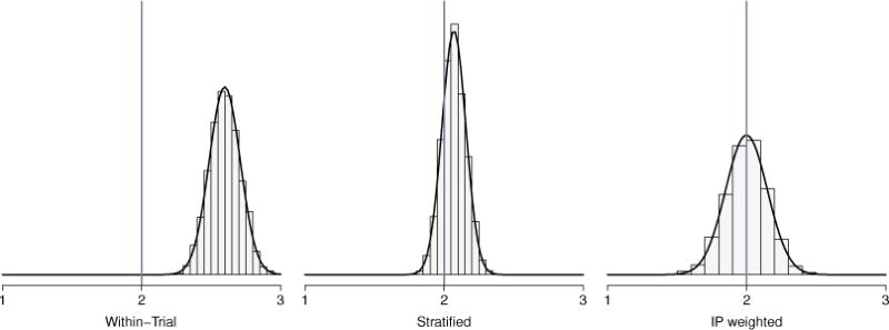
Comparison of the distributions of within-trial estimator ${\widehat{\mathrm{\Delta }}}_T$, stratified estimator ${\widehat{\mathrm{\Delta }}}_S$, and inverse probability of sampling weighted estimator ${\widehat{\mathrm{\Delta }}}_{\mathit{IPSW}}$, based on 5,000 simulated data sets where the sampling score model is correctly specified and Δ = 2 with one continuous covariate, β = (−7, 0.6) and α = 1 (scenario 4).

Simulations were also performed with the sampling score model misspecified. A second covariate was generated for each member of the target population and the true sampling score was w_i = {1 + exp(−β₀ −β₁Z_1i − β₂Z_2i)}⁻¹. For the first two scenarios, Z_2i ∼ Bernoulli(0.6), and for scenarios 3 to 6, Z_2i ~ N(0, 1). For those included in the randomized trial (S_i = 1), X_i was generated as Bernoulli(0.5) and the outcome Y was generated according to Y_i = ν₀+ν₁Z_1i+ν₂Z_2i+ξX_i+α₁Z_1iX_i+ α₂Z_2iX_i+ε_i, ε_i ∼ N(0, 1). For scenarios 1 to 4, (ν₀, ν₁, ν₂, ξ, α₁, α₂) = (0, 1, 1, 2, 1, 1). For scenarios 5 to 6, (ν₀, ν₁, ν₂, ξ, α₁, α₂) = (0, 1, 1, 2, 2, 2). The estimated sampling scores were computed based on a misspecified logistic regression with Z_1i as the only covariate, i.e., ${\widehat{w}}_i={\{1+\exp (-{\widehat{\beta }}_0-{\widehat{\beta }}_1{Z}_{i1})\}}^{-1}$. Two sampling score models were considered: Scenario 1, 3, and 5 set β = (−7, 0.4, 0.4); Scenario 2, 4, and 6 set β = (−7, 0.6, 0.6). Based on the distribution of Z_i = (Z_1i, Z_2i) in the target population, the truth was Δ = 2.8 for scenarios 1 and 2 and Δ = 2 for scenarios 3 through 6.

Comparisons between the IPSW and stratified estimators when the sampling score model was misspecified are summarized in Appendix C Table 1. The bias was reduced by approximately half when either the IPSW or the stratified estimator was employed as compared to the within-trial estimator. The sandwich-type estimator of the variance of the IPSW estimator performed reasonably well when the sampling score model was misspecified; however, CI coverage was below the nominal level.

Lastly, simulations were also performed with reduced overlap in the distribution of Z in the trial and target population. Specifically, the simulation study described above with correct specification of the sampling score model was repeated, except that β₁ = 1 in scenarios 1, 3, and 5, and β₁ = 2 in scenarios 2, 4, and 6. Thus, there was a stronger association between the covariate Z₁ and trial participation than in the original set of simulations, leading to greater differences in the covariate distributions between trial participants and the cohort. For example, in scenario 1, P (Z₁ = 1|S = 1) = 0.40 and P (Z₁ = 1|S = 0) = 0.20 when β₁ = 1, compared to P (Z₁ = 1|S = 1) = 0.26 and P (Z₁ = 1|S = 0) = 0.20 when β₁ = 0.4. Results from this last simulation study are summarized in Appendix C Table 2. The IPSW estimator was unbiased for all scenarios, with the corresponding CI coverage approximating the nominal level except in scenarios 4 and 6. The stratified estimator was biased (although less than the within trial estimator) and the corresponding CIs did not cover at the nominal level except in scenario 1. Because of the reduced overlap in the covariate distributions between the trial and cohort, both the IPSW and stratified estimators were more variable relative to the simulation results in Table 1.

5. Applications

5.1. Trials and Cohorts

In this section, the methods described in Section 3.1 are applied to generalize results from two different ACTG randomized clinical trials, ACTG 320 and ACTG A5202. Two different target populations are considered, namely all women currently living with HIV in the US and all people currently living with HIV in the US.

The ACTG 320 trial examined the safety and efficacy of adding a protease inhibitor (PI) to an HIV treatment regimen with two nucleoside analogues. A total of 1,156 participants were enrolled in ACTG 320 between January 1996 and January 1997 and were recruited from 33 AIDS clinical trial units and 7 National Hemophilia Foundation sites in the US and Puerto Rico. These participants were HIV-positive, highly active antiretroviral therapy (HAART) naive, and had CD4 T cell counts ≤ 200 cells/mm³ at screening. Of the 1,156 participants, 200 were women (Hammer et al., 1997). Among ACTG 320 participants, 116 (10%) were missing the outcome of CD4 count at week 4, so they are excluded from the analysis below. The baseline characteristics of the ACTG 320 participants are shown in Table 2.

Table 2.

Characteristics of WIHS participants, CNICS participants, and ACTG 320 participants at baseline.^a

Variable	WIHS (m = 493)	ACTG 320 Women (n = 200)	CNICS (m = 6,158)	ACTG 320 Men and Women (n = 1,156)
Male sex - %	0	0	80	83
Race or ethnic group - %
White, non-Hispanic	18	31	40	52
Black, non-Hispanic	55	48	44	28
Hispanic	25	21	12	18
Asian/Other	2	1	5	2
Median age - yr (Q1-Q3)b	40 (35-45)	36 (30-42)	41 (34-47)	38 (33-44)
Age group - no. %
[16, 30) yr	7	23	12	12
[30, 40) yr	43	44	34	47
[40, 50) yr	40	27	37	30
[50, ·) yr	10	7	17	11
Injection drug use - %	37	18	20	16
Median CD4 countc (Q1-Q3)	108 (41-172)	82 (26-139)	89 (27-172)	75 (23-137)
Baseline CD4 count - %
(0, 50) cells/mm3	30	36	36	39
[50, 100) cells/mm3	17	22	17	22
[100, 200) cells/mm3	37	37	30	32
[200, ·) cells/mm3	16	6	17	7

^am is the number of participants in the cohort study. n is the number of participants in the trial.

^bQ1 is the first quartile and Q3 is the third quartile.

^cOne ACTG 320 participant was missing CD4 cell count.

The ACTG A5202 trial assessed equivalence of abacavir-lamivudine (ABC-3TC) or tenofovir disoproxil fumarate-emtricitabine (TDF-FTC) plus efavirenz or ritonavir-boosted atazanavir. A total of 1,857 participants were enrolled in A5202 between September 2005 and November 2007 and were recruited from 59 ACTG sites in the US and Puerto Rico. These participants were HIV-positive, antiretroviral (ART) naive, and had viral load > 1,000 copies/ml at screening. Of the 1,857 participants, 322 were women (Sax et al., 2009, 2011). Among A5202 participants, 417 (22%) were missing the outcome of CD4 count at week 48, so they are excluded from the analysis below. The baseline characteristics of the A5202 participants are shown in Table 3.

Table 3.

Characteristics of WIHS participants, CNICS participants, and ACTG A5202 participants at baseline.^a

Variable	WIHS (m = 1,012)	ACTG A5202 Women (n = 322)	CNICS (m = 12,302)	ACTG A5202 Men and Women (n =1,857)
Male sex - %	0	0	82	83
Race or ethnic groupb - %
White, non-Hispanic	17	18	45	40
Black, non-Hispanic	58	53	38	33
Hispanic	22	26	12	23
Asian/Other	3	3	5	3
Median age - yr (Q1-Q3)c	39 (33-44)	39 (31-46)	39 (31-46)	38 (31-45)
Age group - %
[16, 30) yr	12	18	20	22
[30, 40) yr	43	34	34	34
[40, 50) yr	34	33	32	31
[50, ·] yr	11	15	14	14
Injection drug use - %	38	6	17	9
Hepatitis B/C - %	35	8	18	9
AIDS diagnosis - %	37	19	23	17
CD4 countd - %
(0, 50) cells/mm3	10	19	16	18
[50, 100) cells/mm3	6	7	7	8
[100, 200) cells/mm3	16	17	14	17
[200, 350) cells/mm3	29	40	27	35
[350, ·) cells/mm3	39	16	36	22
Median CD4 count (Q1-Q3)	290 (162-423)	226 (87-313)	271 (109, 427)	230 (90-334)
Viral load - %
[0, 50, 000) cp/ml	55	58	52	54
[50, 000, 100, 000)  cp/ml	14	19	15	21
[100, 000, 300, 000)  cp/ml	19	12	18	11
[300, 000, 500, 000) cp/ml	5	3	6	4
[500, 000, ·) cp/ml	7	8	8	10
Median log10 viral load (Q1-Q3)	4.61 (4.04-5.11)	4.58 (4.07-4.93)	4.64 (3.95-5.18)	4.66 (4.33-5.01)

^am is the number of participants in the cohort study. n is the number of participants in the trial.

^bFive A5202 participants were missing race.

^cQ1 is the first quartile and Q3 is the third quartile.

^dOne A5202 participant was missing CD4 cell count.

Data from two cohort studies, WIHS and Center for AIDS Research Network of Integrated Clinical Systems (CNICS), are used in the analysis below to generalize the ACTG 320 and A5202 trial results. Participants in WIHS and CNICS were considered to be representative samples of the target populations, i.e., all women living with HIV in the US and all people living with HIV in the US, respectively. A total of 4,129 women (1,065 HIV-uninfected) were enrolled in WIHS between October 1994 and December 2012 at six US sites (Bacon et al., 2005). The CNICS captures comprehensive and standardized clinical data from point-of-care electronic medical record systems for population-based HIV research (Kitahata et al., 2008). The CNICS cohort includes over 27,000 HIV-infected adults (at least 18 years of age) engaged in clinical care since January 1995 at eight CFAR sites in the US.

For generalizing results from ACTG 320, the analysis included cohort participants who were HIV-positive, HAART naive, and had CD4 cell counts ≤ 200 cells/mm³ at the previous visit (m = 493 women and m = 6,158 men and women combined). For generalizing results from A5202, the analysis included cohort participants who were HIV-positive, ART naive, and had viral load > 1,000 copies/ml at the previous visit (m = 1,012 women and m = 12,302 men and women combined). Table 2 displays the characteristics of the women in the WIHS sample and the participants in the CNICS sample used to generalize results from ACTG 320. Likewise, the characteristics of the women in the WIHS sample and participants in the CNICS sample used to generalize results from ACTG A5202 are displayed in Table 3.

5.2. Analysis

The IPSW and stratified estimators were employed to generalize the difference in the average change in CD4 from baseline between treatment groups observed among women in the trials to all women currently living with HIV in the US and among all participants in the trials to all people currently living with HIV in the US. Based on Centers for Disease Control and Prevention (2012) estimates, the size of the first target population was assumed to be 280,000 women and the size of the second target population was assumed to be 1.1 million people.

The population average treatment effect was estimated using the IPSW estimator in (1). To estimate the sampling scores, the data from the ACTG trial (i.e., 320 and A5202) and cohort (i.e., WIHS or CNICS) were analyzed together, with S = 1 for those in the ACTG trial and S = 0 for those in the cohort. In the model to estimate the sampling scores, the outcome was trial participation and the possible covariates for ACTG 320 included sex, race/ethnicity, age, history of injection drug use (IDU), and baseline CD4 and for ACTG A5202 included sex, race/ethnicity, age, history of IDU, hepatitis B/C, AIDS diagnosis, baseline CD4 and baseline log₁₀ viral load. The variable hepatitis B/C was binary, indicating infection with hepatitis B or hepatitis C or both. Variables associated with trial participation, the outcome, or effect modifiers, as well as all pairwise interactions, were included in the sampling score model. Sex was not included as a covariate in analyses generalizing the trial results among women.

5.3. Results

Estimates of the mean differences based on the within-trial estimator among women and all participants are given in Table 4. Among all participants and among just women in ACTG 320, there was a significant difference in the change in CD4 from baseline to 4 weeks between the PI and non-PI groups. Among women in A5202 at week 48, those randomized to ABC-3TC had an average change in CD4 cell count comparable to those randomized to a regimen with TDF-FTC. Among all participants in A5202, those randomized to ABC-3TC had an average change in CD4 cell count slightly higher than those randomized to a regimen with TDF-FTC, but this did not achieve statistical significance.

Table 4.

Estimated difference in mean change in CD4 cell count^a and corresponding 95% confidence intervals (CIs) in two target populations (all men and women combined and all women living with HIV in the US) based on data from ACTG trials, the WIHS, and CNICS.^b

Cohort	m	Trial	n	Difference in Mean Change (95% CI)
				${\widehat{\mathrm{\Delta }}}_T$	${\widehat{\mathrm{\Delta }}}_S$	${\widehat{\mathrm{\Delta }}}_{\mathit{IPSW}}$
WIHS	493	320c	200	24 (7, 41)	38 (17, 59)	46 (23, 70)
WIHS	1,012	A5202d	322	1 (−35, 37)	−19 (−62, 25)	35 (−45, 115)
CNICS	6,158	320	1,156	19 (12, 25)	18 (9, 26)	17 (9, 25)
CNICS	12,302	A5202	1,857	6 (−8, 20)	7 (−18, 32)	−2 (−31, 28)

^aFor 320, the outcome was change in CD4 cell count from baseline to week 4. For A5202, the outcome was change in CD4 cell count from baseline to week 48.

^bT = within trial; S = stratified; ISPW = inverse probability of sampling weighted.

^cFor 320, the treatment contrast was protease inhibitor (X = 1) vs. no protease inhibitor (X = 0).

^dFor A5202, the treatment contrast was abacavir-lamivudine (X = 1) vs. tenofovir disoproxil fumarate-emtricitabine (X = 0) plus efavirenz or ritonavir-boosted atazanavir.

Table 4 also displays the results for the two ACTG trials generalized to both target populations. In the target population of all women living with HIV in the US, the IPSW estimate was approximately double the within-trial estimate ( ${\widehat{\mathrm{\Delta }}}_{\mathit{IPSW}}=46$ compared to ${\widehat{\mathrm{\Delta }}}_T=24$), suggesting that the within-trial result may underestimate the effects of PIs in all HIV-infected women in the US. The IPSW estimator also indicated a much stronger protective effect of ABC-3TC (vs. TDF-FTC) in the target population of all HIV-infected women in the US ( ${\widehat{\mathrm{\Delta }}}_{\mathit{IPSW}}=35$ compared to ${\widehat{\mathrm{\Delta }}}_T=1$, providing evidence that this particular ART combination may increase CD4 cell counts more on average than what was observed in the trial. In the target population of all people living with HIV in the US, the IPSW estimates were comparable to the within-trial effect estimates, suggesting that both the effect of PIs and the effect of the ART combination ABC-3TC (vs. TDF-FTC) from the trials may be generalizable to all people living with HIV in the US. In summary, these results suggest the ACTG trial results are more generalizable for US men with HIV than US women with HIV.

6. Discussion

In this paper, we considered generalizing results from a randomized trial to a specific target population using inverse probability of sampling weights. The IPSW estimator was shown to be consistent and asymptotically normal and a consistent sandwich-type estimator of the variance was provided. In a simulation study, the IPSW outperformed the stratified estimator when the sampling score was correctly specified. The IPSW was unbiased for all scenarios and the CIs exhibited coverage approximately at the nominal level, except when there was limited overlap in the distribution of covariates in the trial as compared to the target population. With a continuous covariate, the stratified estimator exhibited bias and the corresponding CI had poor coverage, particularly in the presence of stronger effect modification.

In the illustrative example, the ACTG 320 and A5202 trial results appear to be generalizable to all people living with HIV in the US. On the other hand, the within-trial effect estimates among women in the two ACTG trials were not comparable to the effect estimates in the target population of women. This lack of comparability may be explained by differences in the distribution of certain effect modifiers between the trial and the target population. Figures 1-4 in Appendix D show within-trial subgroup effect estimates and CIs for both trials. Among women in A5202, the results in Figure 3 of Appendix D suggest hepatitis B/C, IDU, and age were possible effect modifiers. These three covariates were also associated with trial participation among women, and thus may explain why the A5202 within-trial effect estimate among women was not similar to the IPSW effect estimate in the target population of women. In particular, women with hepatitis B/C were less likely to participate in A5202 and tended to have a greater mean change in CD4. Thus by accounting for hepatitis B/C, we would expect the IPSW estimate to be greater than the within-trial estimate. Likewise, women who were younger or had a history of IDU were also less likely to participate in A5202 and tended to have a greater mean change in CD4 than older women or those without a history of IDU, respectively. Results from both ACTG A5202 and ACTG 320 were not sensitive to the specification of the size of the target population, although some results were sensitive to the specification of the sampling score model (results not shown). In the data example, a complete case analysis was performed; however, in practice, one would want to address the possibility that the missingness was not completely at random.

When applying these methods, the analysis is subject to the following considerations. First, the ignorable trial participation mechanism is a key assumption which supposes participants in the ACTG trials are no different from individuals in WIHS and CNICS with respect to the treatment-outcome relationship conditional on observed covariates. However, it is plausible that there exist unmeasured covariates associated with trial participation and the outcome which confound the association between treatment and outcome even after conditioning on the observed covariates. The methods considered in this paper also assume there are no variations of treatment. Within the context of the HIV treatment trial analysis, this assumption supposes antiretroviral treatment adherence rates were similar among those in the target population and participants in the ACTG trials. This assumption could be assessed if data related to adherence was collected in WIHS, CNICS, and the ACTG trials. The no variations of treatment assumption additionally supposes there are no other behavioral responses or contextual effects (Ding and Lehrer, 2015) of study participation that would not remain if the treatment were adopted in the target population.

In addition, the sampling score model was assumed to be correctly specified (e.g., correct covariate functional forms). Because some degree of model misspecification is inevitable, sensitivity analysis of inferences about the treatment effect in the population to the sampling score model specification is recommended. Similarly, the stratified estimator (Tipton et al., 2014; O’Muircheartaigh and Hedges, 2013) requires that individuals sharing the same stratum of the sampling score distribution can be identified. This estimator may be biased when there is residual confounding within strata and, in general, is not a consistent estimator of the PATE (Lunceford and Davidian, 2004).

The inferential methods considered in this paper assume the cohort to be a random sample (i.e., representative) of the target population. In the HIV application, participants in WIHS (CNICS) are assumed to constitute a random sample of women (men and women) living with HIV in the US. This assumption would be violated if cohort participation is associated with individual characteristics, such as age, living in an urban area, income, employment status, etc. In the context of the HIV application, this assumption might be considered more plausible if the target population were instead defined with greater specificity, e.g., as all women (and men) living with HIV who are in care at the geographical locations which have sites in the cohort studies. If the cohort is not considered representative of the target population, one possibility is weighting the cohort data to the distribution of covariates in a census (e.g., Centers for Disease Control and Prevention (CDC) estimates). A limitation of this approach is that the census may not have covariate information as rich as the cohort data. The CDC estimates used to quantify the size of the target population in the example were for all people living with HIV. Use of surveillance studies that report on the number of ART and HAART naive HIV patients in the US could further sharpen the information about the target population.

In this paper, we consider randomized trials where individuals are independently randomized to treatment or control. Future research could entail extensions to cluster randomized trials wherein clusters of individuals are independently randomized to treatment or control, with all individuals in the same cluster receiving the same randomization assignment. Causal inference methods for individually randomized studies are not necessarily valid for cluster randomized trials (Middleton and Aronow, 2015), such that the methods considered in this paper may not be directly applicable to cluster randomized trials.

Future research could also entail using machine learning methods (Westreich et al., 2010), maximum entropy (Hartman et al., 2015), or flexible regression methods such as Bayesian adaptive tree regression (Chipman et al., 2010) instead of weighted logistic regression to estimate the sampling scores. The IPSW estimator considered in this paper may be highly variable when there is limited overlap in the distribution of the covariates in the trial as compared to the target population. Thus, alternative estimators should be developed for settings where there is limited covariate distribution overlap. Formal sensitivity analysis methods could be developed to assess the extent to which violations of key assumptions, such as the ignorable trial participation mechanism assumption, potentially affect inference about the treatment effect in the target population. Alternatively, bounds could be derived (as in Gechter (2015)) under weaker assumptions which only partially identify the population average treatment effect. For the methods considered in this manuscript, no information on the exposure or outcome is required from the cohort study. In settings where the outcome data is available in the cohort, approaches similar to Hotz et al. (2005) and Hartman et al. (2015) could be developed to test the ignorable trial participation mechanism assumption.

Additional extensions might be considered based on the types of data typical of biomedical, public health, and econometric studies. For example, time-to-event endpoints are common in HIV/AIDS trials, so extensions to accommodate right censored outcomes could be considered. Lastly, in some settings such as infectious disease studies, the treatment or exposure of one individual may affect the outcome of another individual; extensions of existing generalizability methods, such as using inverse probability of sampling weights, to allow for interference would have utility in such settings.

References

- Allcott H. Social norms and energy conservation. Journal of Public Economics. 2011;95:1082–1095. [Google Scholar]
- Allcott H. Site selection bias in program evaluation. The Quarterly Journal of Economics. 2015;130:1117–1165. [Google Scholar]
- Allcott H, Mullainathan S. Tech rep. National Bureau of Economic Research; 2012. External validity and partner selection bias. (Working Paper Number 18373). [Google Scholar]
- Bacon MC, von Wyl V, Alden C, Sharp G, Robison E, Hessol N. The Women’s Interagency HIV Study: An observational cohort brings clinical sciences to the bench. Clinical and Diagnostic Laboratory Immunology. 2005;12:1013–1019. doi: 10.1128/CDLI.12.9.1013-1019.2005. [DOI] [PMC free article] [PubMed] [Google Scholar]
- Carroll RJ, Ruppert D, Stefanski LA, Crainiceanu CM. Measurement Error in Nonlinear Models: A Modern Perspective. New York: CRC Press; 2010. [Google Scholar]
- Chipman HA, George EI, McCulloch RE. BART: Bayesian additive regression trees. The Annals of Applied Statistics. 2010;4:266–298. [Google Scholar]
- Cole SR, Stuart EA. Generalizing evidence from randomized clinical trials to target populations: The ACTG 320 trial. American Journal of Epidemiology. 2010;172:107–115. doi: 10.1093/aje/kwq084. [DOI] [PMC free article] [PubMed] [Google Scholar]
- Centers for Disease Control and Prevention. Diagnoses of HIV infection and AIDS in the United States and dependent areas. HIV Surveillance Report. 2012;17 [Google Scholar]
- Ding W, Lehrer SF. Estimating treatment effects from contaminated multi-period education experiments: The dynamic impacts of class size reductions. The Review of Economics and Statistics. 2010;92:31–42. [Google Scholar]
- Ding W, Lehrer SF. Tech rep. Queen’s University; 2015. Estimating context-independent treatment effects in education experiments. (Working Paper Number 3788). [Google Scholar]
- Gandhi M, Ameli N, Bacchetti P, Sharp GB, French AL, Young M. Eligibility criteria for HIV clinical trials and generalizability of results: The gap between published reports and study protocols. AIDS. 2005;19:1885–1896. doi: 10.1097/01.aids.0000189866.67182.f7. [DOI] [PubMed] [Google Scholar]
- Gechter M. Generalizing the results from social experiments: Theory and evidence from Mexico and India. Department of Economics, Pennsylvania State University; 2015. Unpublished manuscript. [Google Scholar]
- Greenblatt RM. Priority issues concerning HIV infection among women. Women’s Health Issues. 2011;21:S266–S271. doi: 10.1016/j.whi.2011.08.007. [DOI] [PubMed] [Google Scholar]
- Greenland S, Pearl J, Robins JM. Causal diagrams for epidemiologic research. Epidemiology. 1999;10:37–48. [PubMed] [Google Scholar]
- Hammer SM, Squires KE, Hughes MD, Grimes JM, Demeter LM, Currier JS. A controlled trial of two nucleoside analogues plus indinavir in persons with HIV infection and CD4 cell counts of 200 per cubic millimeter or less. New England Journal of Medicine. 1997;337:725–733. doi: 10.1056/NEJM199709113371101. [DOI] [PubMed] [Google Scholar]
- Hartman E, Grieve R, Ramsahai R, Sekhon JS. From sample average treatment effect to population average treatment effect on the treated: Combining experimental with observational studies to estimate population treatment effects. Journal of the Royal Statistical Society: Series A (Statistics in Society) 2015;178:757–778. [Google Scholar]
- Heckman JJ, Urzua S, Vytlacil E. Understanding instrumental variables in models with essential heterogeneity. The Review of Economics and Statistics. 2006;88:389–432. [Google Scholar]
- Hernan MA, VanderWeele TJ. Compound treatments and transportability of causal inference. Epidemiology. 2011;22:368–377. doi: 10.1097/EDE.0b013e3182109296. [DOI] [PMC free article] [PubMed] [Google Scholar]
- Hirano K, Imbens GW, Ridder G. Efficient estimation of average treatment effects using the estimated propensity score. Econometrica. 2003;71:1161–1189. [Google Scholar]
- Hotz VJ, Imbens GW, Mortimer JH. Predicting the efficacy of future training programs using past experiences at other locations. Journal of Econometrics. 2005;125:241–270. [Google Scholar]
- Keiding N, Louis TA. Perils and potentials of self-selected entry to epidemiological studies and surveys. Journal of the Royal Statistical Society: Series A (Statistics in Society) 2016;179:319–376. [Google Scholar]
- Kitahata MM, Rodriguez B, Haubrich R, Boswell S, Mathews WC, Lederman MM. Cohort profile: The Centers for AIDS Research Network of Integrated Clinical Systems. International Journal of Epidemiology. 2008;37:948–955. doi: 10.1093/ije/dym231. [DOI] [PMC free article] [PubMed] [Google Scholar]
- Lunceford JK, Davidian M. Stratification and weighting via the propensity score in estimation of causal treatment effects: A comparative study. Statistics in Medicine. 2004;23:2937–2960. doi: 10.1002/sim.1903. [DOI] [PubMed] [Google Scholar]
- Middleton JA, Aronow PM. Unbiased estimation of the average treatment effect in cluster-randomized experiments. Statistics, Politics and Policy. 2015;6:39–75. [Google Scholar]
- Muller S. Tech rep A Southern Africa Labour and Development Research Unit. Cape Town: SALDRU, University of Cape Town; 2014. Randomised trials for policy: A review of the external validity of treatment effects. (Working Paper Number 127). [Google Scholar]
- O’Muircheartaigh C, Hedges LV. Generalizing from unrepresentative experiments: A stratified propensity score approach. Journal of the Royal Statistical Society: Series C (Applied Statistics) 2013;63:195–210. [Google Scholar]
- Pearl J, Bareinboim E. External validity: From do-calculus to transportability across populations. Statistical Science. 2014;29:579–595. [Google Scholar]
- Robins JM, Mark SD, Newey WK. Estimating exposure effects by modelling the expectation of exposure conditional on confounders. Biometrics. 1992;48:479–495. [PubMed] [Google Scholar]
- Rosenbaum PR, Rubin DB. The central role of the propensity score in observational studies for causal effects. Biometrika. 1983;70:41–55. [Google Scholar]
- Rubin DB. Discussion of “Randomization analysis of experimental data in the Fisher randomization test” by D. Basu. Journal of the American Statistical Association. 1980;75:591–593. [Google Scholar]
- Sax PE, Tierney C, Collier AC, Daar ES, Mollan K, Budhathoki C, Godfrey C, Jahed NC, Myers L, Katzenstein D, et al. Abacavir/lamivudine versus tenofovir DF/emtricitabine as part of combination regimens for initial treatment of HIV: Final results. Journal of Infectious Diseases. 2011;204:1191–1201. doi: 10.1093/infdis/jir505. [DOI] [PMC free article] [PubMed] [Google Scholar]
- Sax PE, Tierney C, Collier AC, Fischl MA, Mollan K, Peeples L, Godfrey C, Jahed NC, Myers L, Katzenstein D, et al. Abacavir–lamivudine versus tenofovir–emtricitabine for initial HIV-1 therapy. New England Journal of Medicine. 2009;361:2230–2240. doi: 10.1056/NEJMoa0906768. [DOI] [PMC free article] [PubMed] [Google Scholar]
- Scott AJ, Wild C. Fitting logistic models under case control or choice based sampling. Journal of the Royal Statistical Society: Series B (Methodological) 1986;48:170–182. [Google Scholar]
- Seaman SR, White IR. Review of inverse probability weighting for dealing with missing data. Statistical Methods in Medical Research. 2013;22:278–295. doi: 10.1177/0962280210395740. [DOI] [PubMed] [Google Scholar]
- Stuart EA, Bradshaw CP, Leaf PJ. Assessing the generalizability of randomized trial results to target populations. Prevention Science. 2015;16:475–485. doi: 10.1007/s11121-014-0513-z. [DOI] [PMC free article] [PubMed] [Google Scholar]
- Stuart EA, Cole SR, Bradshaw CP, Leaf PJ. The use of propensity scores to assess the generalizability of results from randomized trials. Journal of the Royal Statistical Society: Series A (Statistics in Society) 2011;174:369–386. doi: 10.1111/j.1467-985X.2010.00673.x. [DOI] [PMC free article] [PubMed] [Google Scholar]
- Tipton E. Improving generalizations from experiments using propensity score sub-classification: Assumptions, properties, and contexts. Journal of Educational and Behavioral Statistics. 2013;38:239–266. [Google Scholar]
- Tipton E, Hedges L, Vaden-Kiernan M, Borman G, Sullivan K, Caverly S. Sample selection in randomized experiments: A new method using propensity score stratified sampling. Journal of Research on Educational Effectiveness. 2014;7:114–135. [Google Scholar]
- Westreich D, Cole SR. Invited commentary: Positivity in practice. American Journal of Epidemiology. 2010;171:674–677. doi: 10.1093/aje/kwp436. [DOI] [PMC free article] [PubMed] [Google Scholar]
- Westreich D, Lessler J, Funk MJ. Propensity score estimation: Neural networks, support vector machines, decision trees (cart), and meta-classifiers as alternatives to logistic regression. Journal of Clinical Epidemiology. 2010;63:826–833. doi: 10.1016/j.jclinepi.2009.11.020. [DOI] [PMC free article] [PubMed] [Google Scholar]
- Wooldridge JM. Inverse probability weighted M-estimators for sample selection, attrition, and stratification. Portuguese Economic Journal. 2002;1:117–139. [Google Scholar]
- Wooldridge JM. Inverse probability weighted estimation for general missing data problems. Journal of Econometrics. 2007;141:1281–1301. [Google Scholar]
Associated Data
This section collects any data citations, data availability statements, or supplementary materials included in this article.