Development of an attenuation correction method for direct x‐ray fluorescence (XRF) imaging utilizing gold L‐shell XRF photons

Abstract

Purpose

This work proposes a semiempirical correction method for attenuation of x‐ray fluorescence (XRF) photons and/or an excitation beam during direct XRF imaging (i.e., mapping) of gold nanoparticle (GNP) distribution utilizing gold L‐shell XRF photons.

Methods

The current method was first devised by finding the two following relationships: (a) ratio of gold XRF peak intensity (L _α at ~9.7 keV and L _β at ~11.4 keV) vs pathlength of XRF photons; (b) XRF photon counts produced (N _xrf ) vs scattered photon counts produced (N _scat ). Monte Carlo simulations were performed using the Geant4 tool kit to characterize the aforementioned relationships for different tissue‐like media. The applicability of the method was tested experimentally by acquiring 2D L‐shell XRF images of custom‐made phantoms using an experimental benchtop x‐ray fluorescence computed tomography setup.

Results

The results show that the ratio of gold L‐shell XRF peak intensities allowed an estimation of the pathlength of XRF photons, thus can be utilized to correct for attenuation of XRF photons after emission. The results also demonstrate that N _scat , through a proportionality $N_{\mathit{xrf}}\propto N_{\mathit{scat}}^T$ where the exponent T depends on the energy of scattered photons, could be used to correct for attenuation of an excitation beam prior to producing XRF photons. The corrected XRF signal was found independent of the densities of tissue‐like media present along the passage of an excitation beam or emitted XRF photons.

Conclusions

The current results suggest that the developed attenuation correction method plays an essential role for the detection of GNPs on the order of parts‐per‐million, and also for the determination of GNP concentration/location within the imaging object made of tissue‐like media, without any prior knowledge of the imaging object shape, under the conditions deemed relevant to biomedical applications of gold L‐shell XRF‐based imaging.

1. Introduction

Recent experimental studies have demonstrated the feasibility of performing direct x‐ray fluorescence (XRF) imaging (i.e., mapping)^{1, 2} or (rotational) x‐ray fluorescence computed tomography (XFCT)³ of gold nanoparticle (GNP) distribution within small biological samples (e.g., animal tumors less than 1.0 cm in diameter or thickness) using a benchtop polychromatic x‐ray source for excitation of gold L‐shell XRF photons (~9.7 and ~11.4 keV). Compared to its counterpart based on gold K‐shell XRF photons (~67 and ~68.8 keV),^{4, 5, 6, 7} this approach referred to as benchtop L‐shell XRF imaging or XFCT has been shown to provide a much lower GNP (or gold) detection limit, typically on the order of parts‐per‐million (ppm).^{1, 2} This drastic improvement in the detection limit (e.g., by two orders of magnitude) can be attributed to much lower scatter background as well as the availability of x‐ray detector with much higher detection efficiency/energy resolution around gold L‐shell XRF peaks, all of which immensely facilitate the extraction of gold L‐shell XRF peaks from the Compton scatter background.

Despite its high sensitivity, benchtop L‐shell XRF imaging suffers from higher attenuation of gold L‐shell XRF photons compared to its counterpart utilizing gold K‐shell XRF photons. For an accurate quantification of the GNP distribution within the imaging object, therefore, it is necessary to properly correct for attenuation of L‐shell XRF photons as well as an excitation (or incident) x‐ray beam prior to excitation of L‐shell XRF photons.^{1, 2, 8, 9} In previous imaging studies with L‐shell XRF photons, attenuation correction was achieved through either transmission CT images⁸ or the calculation of the ratio of XRF‐to‐Compton scatter counts.^{1, 2} Compared to a relatively straightforward CT image‐based approach (for XFCT), the latter approach (for direct XRF imaging) is based on the fact that the Compton scatter has little dependence on the material density at this energy range; thus, measured Compton scattered photon counts can be used to correct for the attenuation of the excitation beam.^{10, 11} This approach, however, was proposed mainly to correct for self‐absorption in small samples encountered in XRF analysis. Also, it was pointed out that a simple XRF‐to‐Compton scatter ratio might not be sufficient to correct even for self‐absorption, suggesting the use of a power law to further improve the approach.¹² Consequently, when applied to benchtop L‐shell XRF imaging that deals with relatively larger imaging objects with varying shapes (i.e., a wide range of photon pathlengths from the detector's perspective), attenuation correction methods utilizing simple XRF‐to‐Compton scatter ratios become less accurate. In practice, this problem directly hinders accurate imaging of GNP distribution under the realistic scenarios of benchtop L‐shell XRF imaging (or XFCT)¹³ (e.g., ex vivo or in vivo imaging of GNP‐laden subcutaneous xenograft tumors) in which transmission CT imaging is either unavailable or impractical.

The primary goal of this investigation was to develop a robust method that can overcome the aforementioned difficulties in correcting for attenuation of XRF photons as well as an excitation x‐ray beam during L‐shell XRF imaging under the pencil beam (or slit beam) geometry. Due to the difficulty in precisely controlling the key parameters (e.g., pathlengths of XRF photons) experimentally, the currently proposed method was first developed using a Monte Carlo (MC) model of an experimental benchtop XFCT setup. Subsequently, the proposed method was validated experimentally by using L‐shell XRF data obtained from GNP‐loaded symmetrical and asymmetrical phantoms. Additionally, the GNP (or gold) detection limit achievable during L‐shell XRF imaging was determined using the current MC model under the conditions deemed relevant to biomedical imaging, as a function of depth within the phantoms.

2. Materials and methods

2.A. Experimental details

2.A.1. Benchtop XFCT system

The current benchtop XFCT setup (Fig. 1) consisted of a tungsten‐target x‐ray source (MXR‐160/22, COMET Technologies USA, Inc., San Jose, CA, USA) and a silicon drift x‐ray detector (SDD) (XR‐100SDD, Amptek Inc., Bedford, MA, USA) for excitation of XRF photons and detection of them (at 90° with respect to the excitation beam direction), respectively. The source was operated at 60 kVp tube voltage and 45 mA tube current with a focal spot size of 5.5 mm (DIN EN 12543). The beam was filtered using 0.07 mm Cu followed by 0.8 mm Al. This filtration was chosen (based on measurements using different combinations of filter material and thickness) to completely suppress tungsten L _β peak which would overlap with gold L _α peak at 9.7 keV (See Section 3.A for the related result). The filtered excitation beam was collimated by a 5.0‐mm‐thick lead block with an aperture size of 0.5 mm × 1.0 mm, placed ~8.5 cm away from the tungsten‐target. The centers of the imaging phantoms were positioned at 15 cm from the tungsten‐target, where the beam size measured using radiochromic films was 2.0 mm (width) × 4.0 mm (height). The SDD was placed at 4.64 cm from the center of imaging phantoms. For direct XRF imaging/mapping of the phantoms [Fig. 1(a)], the SDD was placed behind a 2.54‐cm‐thick stainless steel detector collimator with a 1.0‐mm‐diameter aperture.

Figure 1.

Top view of the current benchtop XFCT setup. (a) Direct XRF imaging/mapping mode with an inset illustrating the pathlengths of a slit‐type excitation beam (d _exc ) and emitted XRF & scattered photons (d _em ) within the GNP‐loaded phantom, (b) Top view of three phantoms used in the current study: 1.0 cm × 1.0 cm × 1.0 cm cubic phantom (left), arbitrary‐shaped phantom with 5.0‐mm‐diameter inner cavity (middle), calibration phantom with 1.8‐mm inner cavity (right). All phantoms have the same height of 1.0 cm. [Color figure can be viewed at wileyonlinelibrary.com]

2.A.2. Phantoms

The phantoms [Fig. 1(b)] used in this study were custom‐made of polymethyl methacrylate (PMMA, density of 1.18 g cm⁻³) using 3D printers. Three types of phantoms were used for the studies: (a) cylindrical phantoms [Fig. 1(b) right] of 1.8 mm in inner diameter (wall thickness of 0.3 mm) and 1.0 cm in height, an arbitrary‐shaped phantom [Fig. 1(b) middle] consisted of an inner cavity of 0.5 cm in diameter and 1.0 cm in height, and a cubic phantom [Fig. 1(b) left] of dimensions 1.0 cm × 1.0 cm × 1.0 cm and wall thickness of 0.3 mm.

2.A.3. GNP solutions

Varying concentrations of GNPs (AuroVist™—15 nm, Nanoprobes Inc., Yaphank, NY, USA) ranging 10–1000 ppm (i.e., 10 μg Au/mL—1 mg Au/mL) were prepared in phosphate‐buffered saline (PBS) using a serial dilution method from a stock solution of 4.0 wt. % (as provided by the manufacturer). During the preparation of GNP solutions, volumetric measurements were performed using Clip‐Tip variable volume Single Channel Pipettes (1–10 μL with inaccuracy ±1.0%, 10–100 μL with inaccuracy ±0.8%, and 100–1000 μL with inaccuracy ±0.6%, Model 4701140N, ThermoFisher Scientific, Waltham, MA, USA).

2.A.4. Measurement of the excitation beam spectra

The excitation beam spectra from the x‐ray source were measured by placing the detector, in conjunction with a 25.0‐cm‐thick lead collimator (the length of the collimator was kept exceptionally long to avoid saturating the detector by a direct beam) of gradually decreasing hole‐diameter, along the excitation beam axis at ~1.5 m distance away from the tungsten‐target. For these measurements, a CdTe x‐ray detector (XR‐100T‐CdTe, Amptek Inc., Bedford, MA, USA) was used, as the photon counting efficiency of the SDD decreases sharply at energies >10 keV and reaches ~10% at 30 keV. The beam was measured either unfiltered or filtered via 0.07 mm Cu followed by 0.8 mm Al. The acquired raw x‐ray spectra (counts vs channels) were first converted into energy spectra (counts vs energy) using the calibration curves obtained in‐house using isotope‐based check sources and XRF‐producing elements. The acquired x‐ray spectra were also corrected for the photon counting efficiency of the CdTe detector as well as for the so‐called escape events¹⁴ using an MC‐based stripping correction algorithm described elsewhere.¹⁵

2.A.5. Phantom scanning and data acquisition

For the system calibration, XRF spectra (including the scattered photon background) were measured from cylindrical phantoms [Fig. 1(b), right] filled with 10–1000 ppm GNP solutions using 60 s acquisition time for each phantom. To determine the parameters required for the proposed attenuation correction method, a cubic phantom [Fig. 1(b), left] filled with 1000 ppm GNP solution was scanned using the current benchtop XFCT setup. To test the applicability of the proposed attenuation correction method under a more realistic condition, an arbitrary‐shaped phantom [Fig. 1(b), middle] was filled with 1000 ppm GNP solution and scanned. The phantom scans were performed using only translational movements of the phantom and detectors in perpendicular directions (Fig. 1). Both the detector and the phantom were translated (Fig. 1) in 1.0‐mm steps using motorized stages with 60 s acquisition time at each position. For example, the data acquisition time required for the complete scan of an arbitrary‐shaped phantom was (14 × 14 × 60 s=) 196 min.

2.B. Formulation of the attenuation correction method

2.B.1. Formulation

Considering the experimental conditions presented with the direct XRF imaging/mapping mode [Fig. 1(a)] of the current benchtop XFCT system, the three assumptions described below can be made for the attenuation correction method proposed in this study. First, the detected XRF/scatter x‐ray spectra include at least two L‐shell XRF peaks (mixture of one/several lines) whose peak intensities differ only by the fraction f of the photon emission rates and the associated attenuation coefficients.¹⁶ This assumption is true if both XRF peaks are emitted from the same element. Second, the XRF photons from the two XRF peaks are emitted from the same physical location in the imaging area, so that they travel the same pathlength through the media between the point of emission and the detector. This condition can be approximately valid if the beam size is narrow enough (compared to the object/sample size), i.e., the proposed attenuation correction method is limited to the narrow pencil/slit type excitation beam geometry. Third, the attenuation coefficients for the two XRF peak energies are significantly different. This is mostly true for energies below 30 keV, hence the proposed attenuation correction method is generally limited to L‐shell XRF imaging in the case of gold/GNPs.

Let N _α and N _β be the detected XRF photon counts from two gold L‐shell XRF peaks L _α (sum of all inseparable L _α peaks, e.g., L _α1 and L _α2 for gold) and L _β (sum of all inseparable L _β peaks, e.g., L _β1 to L _β4 for gold), respectively and the respective attenuation coefficients are μ _α and μ _β . Also, let d _exc is the pathlength (inside the imaging object) of an excitation beam before hitting the detection line (field of view of the detector collimator) and d _em is the pathlength of emitted XRF and Compton scattered photons before exiting the imaging object. Thus, for a fixed d _exc , the ratio of two XRF peak intensities, referred to as R, can then be formulated using Beer–Lambert law as:

$$R=\frac{N_{\alpha }(d_{\mathit{em}},{\mu }_{\alpha },\rho )}{N_{\beta }(d_{\mathit{em}},{\mu }_{\beta },\rho )}=\frac{N_{\alpha }(0)e^{-{\mu }_{\alpha }\rho d_{\mathit{em}}}}{N_{\beta }(0)e^{-{\mu }_{\beta }\rho d_{\mathit{em}}}}=R_0{e}^{-({\mu }_{\alpha }-{\mu }_{\beta })\rho d_{\mathit{em}}}$$ (1)

Here, $N_{\alpha }(0)$ and $N_{\beta }(0)$ refer to the number of L _α and L _β XRF photons emitted at the excitation point (unattenuated after emission) and $R_0$ is the reference XRF peak intensity ratio defined as $R_0=R\left(d_{\mathit{em}}\cong 0\right)=\frac{N_{\alpha }(0)}{N_{\beta }(0)}$. In principle, $R_0=\frac{{\sum }_i{f}_{\alpha i}^L}{{\sum }_j{f}_{\beta j}^L}$, i.e., the ratio of the total relative fluorescence intensities of all L _α peaks to that of all L _β peaks,¹⁶ which can be readily found from x‐ray data tables.^{17, 18, 19} For example, for pure gold, based on the approximate XRF intensities, $R_0=(90+10)/(100+10+25+20)=0.65$. Thus, we can easily calculate d _em by rewriting Eq. (1) as:

$$d_{\mathit{em}}=\frac{1}{\left({\mu }_{\alpha }-{\mu }_{\beta }\right)\rho }ln{R}_0/R$$ (2)

Finally, the measured XRF and scattered photon counts $N_E(d_{\mathit{em}},{\mu }_E,\rho )$ at any energy E can be corrected for attenuation after emission by using the estimated pathlength to obtain the unattenuated photon count $N_E(0)$ as follows:

$$N_E(0)=N_E(d_{\mathit{em}},{\mu }_E,\rho )exp\left(\frac{{\mu }_E}{{\mu }_{\alpha }-{\mu }_{\beta }}ln{R}_0/R\right)$$ (3)

For the attenuation correction of an excitation beam, the relationship between total XRF photon counts produced ($N_{\mathit{xrf}}$) and Compton scattered photon counts produced ($N_{\mathit{scat}}$) can be described by a simple power law $N_{\mathit{xrf}}\propto N_{\mathit{scat}}^T$.¹² This formula, in its actual form is probably most appropriate for extremely thin analytical samples where the XRF/scatter photons, once produced, suffer from insignificant attenuation before reaching the detector. In case of imaging an area of relatively larger size, e.g., ~1 cm × 1 cm, clearly this condition is not met, hence, the photon counts need to be first corrected for attenuation after emission. Thus, the corrected XRF signal (dimensionless) denoted by S, which is the quantity of interest, is given by Eq. (4).

$$S=\frac{N_{\alpha }\left(0\right)+N_{\beta }\left(0\right)}{N_{\mathit{scat}}^T\left(0\right)}$$ (4)

The procedure that needs to be employed to estimate the parameters of the attenuation correction method are summarized as follows:

XRF/scattered photon counts

The energy ranges over which N _α and N _β are accumulated must be spectrally separated, e.g., 9.4–10.0 keV and 11.0–12.0 keV, respectively for gold. The background counts (Compton scattered photon counts plus electronic noise) at the XRF energies need to be estimated using an appropriate fitting function (which depends on filtering, electronic noise, etc.) and subtracted from N _α and N _β . N _scat can be determined at an energy where it is statistically the most significant, e.g., N _scat  = N _30keV (accumulated over 29.5–30.5 keV) for the current excitation beam and detection geometry.

Attenuation coefficients

μ _α , μ _β , and μ _scat need to be estimated from the reference data or experimentally (over the chosen energy ranges) for water at the gold L‐shell XRF energies as the GNP solutions or GNP‐loaded tumors are mostly water‐like. As noted in Eqs. (1) and (3), if the imaged media is denser than water, the reduced photon count $N_E\left(d_{\mathit{em}},\rho ,{\mu }_{\alpha }\right)$ is compensated by a resultant smaller value of R.

Exponent T

T can be determined by finding a correlation between the unattenuated scattered photon counts (at the chosen scattered photon energy) and the unattenuated XRF photon counts, over varying excitation beam intensity or attenuation pathlength (d _exc ). In practice, the photon spectrum containing such unattenuated photon counts can be obtained experimentally or via MC simulation by irradiating a calibration phantom [e.g., 1.8‐mm‐diameter cylindrical phantom used in the current study, Fig. 1(b)], which is small enough so that the attenuation after photon emission can be ignored, after passing the excitation beam through varying thicknesses of a known tissue‐like material. Once the unattenuated photon counts have been obtained, T can finally be determined from a power law fit to the curve (XRF vs scattered photon counts over varying excitation beam intensity or d _exc ). The results based on the approach described above are presented in Section 3.A.4.

For a given data acquisition time or dose, GNP concentration C, and pathlengths d _exc and d _em , the statistical uncertainty in S can be estimated using the error propagation formula for uncorrelated variables²⁰ as shown in Eq. (5):

$$u_S^2(C,d_{\mathit{exc}},d_{\mathit{em}})=\sum _i{\left(\frac{\partial S}{\partial N_i}{\sigma }_{N_i}\right)}^2+C^2{\sigma }_m^2$$ (5)

Here, N _i refers to N _α , N _β , and N _scat , and ${\sigma }_{N_i}$ refers to their associated uncertainties ${\sigma }_{N_{\alpha }},{\sigma }_{N_{\beta }}$ and ${\sigma }_{N_{\mathit{scat}}}$, respectively, following Poisson statistics (square root of the corresponding counts). The σ _m refers to the uncertainty in the slope of the calibration curve (m), which is generally a linear equation ($S=mC$).

2.B.2. Comparison with other attenuation correction methodologies

The ability to correct XRF images for attenuation was tested in four different ways: (a) using a priori information of the phantom geometry/structure, (b) using a conventional approach based on the XRF‐to‐Compton ratio, (c) using the XRF‐to‐Compton ratio raised to power T, and (d) using the XRF peak ratio‐based method proposed in this study (Section 2.B.1). The performance of each attenuation correction method was evaluated based on the absolute photon counts and the image flatness ($=\frac{N_{\mathit{max}}-N_{\mathit{min}}}{N_{\mathit{max}}+N_{\mathit{min}}}\times 100\%)$ over the central 3 mm × 3 mm region.

2.C. Monte Carlo studies

2.C.1. Monte Carlo model

A MC model (Fig. 2) of the benchtop XFCT system was developed using the Geant4 (release 10.3) toolkit.^{21, 22, 23} The MC model simulated the following processes: generation of x‐rays from the tungsten‐target, filtration of these x‐rays, and irradiation of GNP‐loaded phantoms followed by detection of XRF (and scattered) photons. All dimensions and materials used in the model matched those of the actual components within the current benchtop XFCT system. The detectors were modeled using CdTe and Si materials. For the CdTe detector, the stripping correction algorithm¹⁵ for escape events was applied in the excitation beam spectra measurements. To match the energy resolution of the measured spectra, the simulated spectra were convoluted with the detector response functions (Gaussian with exponential tail), following the approach previously developed.¹⁵ At the tungsten or gold L‐shell XRF energies (~9.7 keV), the response of both detectors was nearly Gaussian (~190 eV full width at half maximum (FWHM) for Si and ~522 eV FWHM for CdTe at 9.7 keV) with little hole tailing for CdTe.

Figure 2.

Geant4 model of the XRF imaging system where simulation was performed in stages of x‐ray generation via bombardment of a 60 keV electron beam onto W‐target and filtration using Cu and Al filter. The filtered pencil beam (1.8‐mm diameter) passed through attenuating media was used to excite GNP solution (1.8‐mm inner diameter and height) surrounded by attenuating media. [Color figure can be viewed at wileyonlinelibrary.com]

The particles were transported using the Penelope electromagnetic physics list. Photoelectric effect, Compton scattering, and Rayleigh scattering were included for photon transport, whereas multiple scattering, Coulomb scattering, ionization, and bremsstrahlung x‐ray production were included for electron transport. Different production thresholds or range cuts were applied to different components within the current MC model, while ensuring that photons produced with their energy above 1.0 keV were always transported.

2.C.2. Validation of x‐ray spectra

The unfiltered/filtered x‐rays were scored [Fig. 2(a)] over a circular disk of 1 mm² at a distance 1.5 m away from the focal spot on the W‐target. One hundred billion particle histories were used for these simulations. For the production and detection of XRF photons from GNPs [Fig. 2(b)], filtered spectra scored at the previous simulation were used for excitation ignoring the additional attenuation in air over 1.5 m compared to that encountered within 15 cm (focal spot‐to‐phantom distance).

2.C.3. Investigation of photon attenuation

To investigate attenuation of an excitation beam and emitted XRF photons, irradiation of cylindrical PMMA tubes (1.8 mm inner diameter) filled with GNP solutions (1000 ppm) by the 60 kVp 1.8‐mm‐diameter filtered pencil beam was simulated. The excitation beam and/or the emitted photons were transmitted through one of the following materials (placed in front of the GNP tube for an excitation beam or placed between the GNP tube and the detector for emitted photons): adipose tissue (density of 0.92 g cm⁻³), water (density of 1.0 g cm⁻³), and blood (density of 1.06 g cm⁻³), with a thickness (i.e., pathlength d _exc or d _em ) ranging 0–1.0 cm. The scored XRF photon counts experienced attenuation in different media and were corrected for attenuation using Eq. (4) with ρ and μ's for water, regardless of the media traversed.

2.C.4. Determination of the detection limit

Additional simulations were performed to score x‐ray spectra at varying GNP concentrations at different pathlengths (d _em  = d _exc for simplicity). Based on these data, the detection limit, defined here as the GNP concentration at which the XRF signal [Eq. (4)] can be measured with at least 68% confidence, was estimated at different pathlengths.

To find the correlation between the number of simulated particles and acquisition time in the benchtop XFCT system, 1.8‐mm (inner) diameter (1.0‐cm height) tube filled with 1000 ppm GNP solutions were excited using the increasing numbers of particles and the detected XRF photon counts were correlated. It was observed that 60 billion filtered simulated particles resulted in the same XRF photon counts as measured in the benchtop XFCT system for 60 s irradiation. To determine the detection limits, GNP tubes were excited using 60 billion filtered particles. Hence, the detection limits obtained from MC simulations should be comparable to what would be expected from 60 s irradiation in the benchtop XFCT system.

3. Results

3.A. Monte Carlo studies

3.A.1. Monte Carlo model validation

The photon spectra obtained from the current MC model were first compared with those from measurements with the 60 kVp beam at three stages as shown in Fig. 3: unfiltered (except inherent filtration through the Be window) beam [Fig. 3(a)] measured using the CdTe detector, filtered (Cu plus Al filter) beam [Fig. 3(b)] measured using the CdTe detector, and photon spectra (XRF + scattered) from a 1.8‐mm‐diameter cylindrical tube containing 1000 ppm GNP solution irradiated by the filtered beam measured using the SDD [Fig. 3(c)]. All simulated spectra including the XRF peak positions agreed with the measured spectra reasonably well (R > 0.95). In the case of SDD‐measured spectrum, some discrepancies can be observed at higher energies (>40 keV) most probably due to poor efficiency of the Si detector > 30 keV [Fig. 3(c)]. The validated MC model enabled a series of controlled studies, for example, precisely varying the pathlengths of an excitation beam as well as emitted XRF photons, which is difficult to perform experimentally.

Figure 3.

Comparison between measured and MC‐calculated photon spectra (normalized by the total area under the spectra). (a) unfiltered 60 kVp beam measured using CdTe detector along the excitation beam axis, (b) 60 kVp beam filtered using ~0.07 mm Cu and 0.8 mm Al measured using CdTe detector along the excitation beam axis, and (c) photon (XRF + scatter) spectrum from a cylindrical tube containing 1000 ppm GNP solution, as measured by SDD placed perpendicular to the excitation beam axis. [Color figure can be viewed at wileyonlinelibrary.com]

3.A.2. Spectrum analysis

The simulated photon spectra from GNP solutions excited by the 60 kVp filtered beam and attenuated by water (Section 2.C) are shown in Fig. 4, where Fig. 4(a) shows the spectra at a few exemplary pathlengths of d _exc or d _em and Fig. 4(b) shows the decrease in the scored XRF (N _α and N _β ) and scattered photon counts (N _30 keV ) as a function of d _exc and d _em . Here, in order to minimize the Poisson noise, the scattered photon counts (N _30 keV ) were estimated around the photon energy (30 keV) corresponding to the maximum scattered photon counts under the current experimental condition. The monotonic reduction (within uncertainty) of XRF photon counts due to the attenuation of an excitation beam can be characterized in terms of a decrease in the scattered photon counts (quantified in Section 3.A.4). The exponential decrease in the detected photon counts (for a given excitation beam intensity), after passage through different pathlengths in water (quantified for other materials in Section 3.A.3), can be characterized by the attenuation coefficients (5.71 ± 0.05) cm⁻¹, (3.47 ± 0.04) cm⁻¹, and (0.35 ± 0.01) cm⁻¹ for $L_{\alpha }$, $L_{\beta }$ and 30 keV (Compton), respectively, as expected theoretically.

Figure 4.

(a) Simulated XRF and scattered photon spectra showing a decrease in detected photon counts due to the attenuation of an excitation beam and emitted XRF photons as a function of the respective pathlengths d _exc or d _em in water, considering d _exc  = 0.2, 0.4, or 0.6 mm for d _em  = 0 and d _em  = 0.2, 0.4, or 0.6 mm for d _exc  = 0. (b) Decrease in XRF or scattered photon counts as a function d _exc (top) or d _em (bottom). [Color figure can be viewed at wileyonlinelibrary.com]

3.A.3. Attenuation of XRF and scattered photons

Figure 5(a) shows the independence of XRF peak intensity ratio R [Eq. (1)] on GNP concentration and pathlength of an excitation beam (d _exc ) in water, while Fig. 5(b) shows the dependence of R on pathlength of emitted photons (d _em ) within different media. R is independent of GNP concentration or d _exc , with the weighted (by standard deviation of data points) mean value of R ₀  = 0.69 ± 0.06, as would be expected theoretically (Section 2.B). R decays exponentially as a function of d _em with faster rates within denser media. The estimated decay constants (1.2 ± 0.1 cm⁻¹ in adipose tissue, 2.2 ± 0.2 cm⁻¹ in water, and 2.4 ± 0.2 cm⁻¹ in blood where the values following ± indicate the fitting uncertainty) are essentially identical to the values of $({\mu }_{\alpha }-{\mu }_{\beta })\rho$ for the respective media, agreeing with the formulation shown in Eq. (1). Hence, $d_{\mathit{em}}$ can be calculated directly from $R(d_{\mathit{em}},\rho )$ using Eq. (2) and XRF photons can be corrected for attenuation after emission using Eq. (3).

Figure 5.

Independence of XRF peak intensity ratio R on GNP concentration and pathlength of an excitation beam (d _exc ) in water (left), and dependence of R on pathlength (d _em ) of emitted XRF photons and the traversed medium (right). [Color figure can be viewed at wileyonlinelibrary.com]

3.A.4. Attenuation of an excitation beam

The XRF photon counts (total counts from two gold L‐shell peaks), unattenuated after emission, are shown in Fig. 6 as a function of corresponding scattered photon counts (in the range 29.5–30.5 keV), where only the excitation beam was attenuated in media over varying pathlengths ($d_{\mathit{exc}}=0-1.0\text{cm})$. The data were fitted using a power law formulae of the type $y=a{x}^T$ and, within the fitting uncertainty, T (1.73 ± 0.10 in adipose tissue, 1.76 ± 0.20 in water, and 1.76 ± 0.18 in blood) was independent of the material density for the tested tissue‐like media. Based on the regression analysis, the relationship observed between the unattenuated XRF vs unattenuated scattered photon counts can also be established as linear as the adjusted R ² was comparable for the two fitting (on average R ²  = 0.983 for power law and 0.980 for linear fitting). Besides, the values of T calculated for different GNP concentrations were found to be constant. Further analysis showed that T was inversely proportional to the mass attenuation coefficient at the energy of scattered photon counts N _scat , varying from 1.0 to 2.0 for the energy range 20–30 keV agreeing with Livingstone.¹²

Figure 6.

Correlation (fitted using $y=a{x}^T)$ between unattenuated XRF and scattered photon counts (cumulative counts in the range 29.5–30.5 keV), where only the excitation beam was attenuated in media over varying pathlengths (0–1.0 cm). Note, as indicated in the plot, the maximum and minimum photon counts occur at d_exc = 0 and 1 cm, respectively. The error bars indicate the standard deviation of counts. [Color figure can be viewed at wileyonlinelibrary.com]

3.A.5. Corrected XRF signal

The corrected XRF signals for different media are shown in Fig. 7. Within the estimation uncertainty, they were found independent of the material density and the pathlength travelled. Despite the uncertainty of the corrected signal being large for d _em  > 0.5 cm (pathlength at which the total XRF photon counts are attenuated by >90%), the corrected XRF signal was constant (the standard deviation (1σ) of the mean XRF signal is 1.3% among 54 data points).

Figure 7.

Corrected XRF signal for different pathlengths of an excitation beam (d _exc ) or emitted XRF photons (d _em ) travelled through different tissue‐like media. [Color figure can be viewed at wileyonlinelibrary.com]

3.A.6. GNP (or gold) detection limit vs pathlength

Figure 8 shows the estimated GNP detection limits potentially achievable at different pathlengths using the current benchtop XFCT system. Here it is assumed that GNPs are located inside water‐like materials and detected with 60 s acquisition time under the current experimental conditions. The detection limit at a given $d_{\mathit{exc}}=d_{\mathit{em}}$ was determined as explained earlier (Section 2.C.4). As would be expected, the detection limit increases exponentially as the pathlength of the excitation/emitted photon increases, thus sets the limit of imaging area accordingly at a given GNP concentration.

Figure 8.

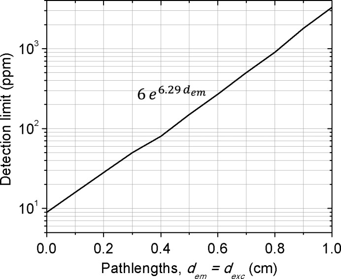
GNP (or gold) detection limit (with 68% confidence) as a function of pathlength when d _exc  = d _em under the current experimental conditions. The results were obtained from MC simulations based on the current experimental setup with a single detector (Fig. 1).

3.B. Experimental studies

3.B.1. Determination of parameters for attenuation correction

To test the applicability of the proposed attenuation correction method for experimental L‐shell XRF imaging, the required parameters (μ's, R ₀ , and T) were determined first based on a scan of a 1.0 cm × 1.0 cm × 1.0 cm phantom filled with 1000 ppm GNP solution using the current benchtop XFCT system. Figure 9 shows the results where all images span 1.0 cm × 1.0 cm cross‐section of the phantom (d _em and d _exc increasing in the left‐to‐right and the bottom‐to‐top directions, respectively). Details about the determination of parameters and their use in the attenuation correction process are presented below.

Figure 9.

Estimation of parameters of the attenuation correction method using a 1.0 cm × 1.0 cm × 1.0 cm phantom filled with 1000 ppm GNP solution. Uncorrected photon counts: (a) N _α , (b) N _β , and (c) N _{30 keV} . The XRF peak intensity ratio R = N _α /N _β is shown in (d). After correction for attenuation of emitted photons: (e) total XRF photon counts and (f) scattered photon counts. The optimum XRF‐to‐scatter ratio found based on (e)–(f) and Eq. (4) is shown in (g). The corrected XRF signal is shown in (h) and its distribution is shown in (i) along with total uncorrected XRF photon counts. [Color figure can be viewed at wileyonlinelibrary.com]

The raw images of photon counts N _α [Fig. 9(a)], N _β [Fig. 9(b)] and N _30keV [Fig. 9(c)] display the exponential attenuation of emitted XRF and scattered photon counts with increasing d _em . Decrease in XRF and scattered photon counts due to attenuation of an excitation beam can be realized noticing a distorted shape of the contours along d _exc . The average photon counts (averaged over all rows) over the d _em range of 0.2–0.8 cm (avoiding the edges) were fitted using exponential functions and the estimated linear attenuation coefficients (${\mu }_{\alpha }=(5.5\pm 0.5){\text{cm}}^{-1}$, ${\mu }_{\beta }=(3.5\pm 0.2){\text{cm}}^{-1}$, and ${\mu }_{30keV}=(0.4\pm 0.1){\text{cm}}^{-1}$) agreed with the commonly accepted values.

As was demonstrated from the simulated data (Fig. 5), the XRF peak intensity ratio R [Fig. 9(d)] decreases with an increase in d _em but stays constant along d _exc . The average value of R over the first column (d _em  ≈ 0) defined as R ₀ was 0.79 ± 0.04. One can also estimate R ₀ based on a single measurement from a calibration phantom [Fig. 3(c)].

The total XRF and scattered photon counts, corrected for attenuation after emission, are shown in Figs. 9(e) and 9(f), respectively. Since the GNP distribution was uniform in this phantom, S in [Eq. (4)] was calculated based on these corrected images with different T and the image flatness was found minimum at $T=1.73$ [Fig. 9(g)], agreeing with that estimated from MC simulations (Section 3.A.4).

Finally, the corrected XRF signal is shown in Fig. 9(h). Distributions of the corrected XRF and uncorrected XRF counts, both normalized to their respective mean values, are shown in Fig. 9(i). In comparison with a biased (decaying) exponential‐type distribution of counts before correction, the corrected signals display an unbiased Gaussian distribution (with a standard deviation of 0.19 ± 0.01, where the value following ± indicates fitting uncertainty). Therefore, one can scan such a simple control phantom to estimate the attenuation correction parameters to characterize a particular configuration of the system and use them for subsequent imaging.

3.B.2. System calibration

Figure 10 shows the measured and MC‐simulated calibration curves of XRF signal as a function of GNP concentration down to 10 ppm. The experimental data were acquired using 60 s acquisition time and the MC‐simulated data were obtained using 60 billion filtered particles. The error bars for experimental data show standard deviation of the mean signal based on five repeated measurements, whereas those for MC data show estimated statistical uncertainty (Section 2.B). Linear response (R ²  > 0.98) was observed for both sets of data, with calibration factor of (8.9 ± 0.4) × 10⁻⁵ ppm⁻¹ for experiment and (9.5 ± 0.2) × 10⁻⁵ ppm⁻¹ for simulation.

Figure 10.

Calibration of corrected XRF signal as a function of GNP concentration (for measurements, acquisition time was 60 s and for MC simulation, 60 billion filtered particles were used). For measurements, the error bars indicate standard deviation (1σ) of mean corrected signal based on five repeated measurements and for simulation, they indicate estimated uncertainty using error propagation as in Eq. (5). [Color figure can be viewed at wileyonlinelibrary.com]

3.B.3. Determination of GNP distribution

Figure 11 illustrates the applicability of the proposed attenuation method under a more realistic condition (e.g., XRF imaging of a small superficial animal tumor) — when the shape of the imaging object is asymmetrical (or difficult to know in advance) and high spatial resolution is desired. Figures 11(a)–(e) show the results of direct XRF imaging, i.e., GNP maps, uncorrected for attenuation, corrected using a priori or known true geometry of the phantom, corrected for attenuation using the XRF‐to‐Compton ratio, corrected using the XRF‐to‐Compton ratio raised to power T (=1.73), and corrected using the currently proposed method, respectively. The mean photon counts at the central region and the associated flatness are summarized in Table 1 . Overall, if the image corrected using a priori information is considered a true XRF map, the two attenuation correction methods based on the XRF‐to‐Compton ratio are found ineffective. For example, they result in a decreased image intensity (~85% of photon counts are lost) or a worse image flatness (about thrice worse than the true XRF map). When the image is corrected using the proposed XRF peak ratio‐based method, the mean photon counts are within 5% of the true XRF map and the image flatness is only ~20% worse.

Figure 11.

Imaged GNP distribution (1000 ppm) inside the phantom as shown in Fig. 1 (the horizontal and vertical axes show the image dimensions in millimeters and the colorbar indicates photon counts). The outer shape of the phantom from solid work drawing is delineated by the asymmetric contour and the inner cylindrical hole of 5.0 mm diameter is shown with a circular contour at the center. (a): the uncorrected image, (b): the image corrected using a priori shape of phantom (using the asymmetric outer contour), (c): the image corrected for attenuation using XRF‐to‐Compton ratio, (d): the image corrected using the XRF‐to‐Compton ratio raised to power T (=1.73), and (e): the image corrected using the proposed method. For all cases, normalized (to its maximum value in the image) Compton photon counts were used for correction. [Color figure can be viewed at wileyonlinelibrary.com]

Table 1.

Effectiveness of the tested attenuation correction methods based on the central 3 mm × 3 mm region of Fig. 11. The values following ± in photon counts indicate the standard deviation of mean counts. The image corrected using a priori information was considered as the Expected image

Correction method	Photon counts		Flatness
	Observed	Observed/expected	Observed	Observed/expected
No correction	774 ± 81	12%	14.4%	2.9
A priori information	6731 ± 206	100%	5.0%	1.0
XRF‐to‐Compton	928 ± 91	14%	14.1%	2.8
(XRF‐to‐Compton)1.73	1074 ± 103	16%	14.9%	3.0
XRF peak ratio	6414 ± 214	95%	6.0%	1.2

4. Discussion

The proposed attenuation correction method was demonstrated to work well for direct L‐shell XRF imaging, in terms of determining the spatial distribution and concentration of GNPs, regardless of the material densities of tissue‐like media. Especially, it can be emphasized that the current investigation was performed under the conditions relevant to possible biomedical applications of direct L‐shell XRF imaging. For example, the current results suggested that the GNP (gold) detection limit less than ~10 ppm over a few mm depths (i.e., at superficial locations within an imaging object involving near zero attenuation, from a practical point of view) would be achievable, while limiting the data acquisition time no more than 60 s at each position/projection which is deemed acceptable for ex vivo imaging of tumor samples and might also allow in vivo imaging of superficial animal tumors dependent on the spatial resolution requirement. Due to significant attenuation of gold L‐shell XRF photons, however, it will be necessary to use at least two (or multiple) opposing detectors or rotate the imaging object in case of a single detector system, in order to achieve the ppm‐level detection limit throughout the imaging object (e.g., animal tumor) during ex vivo or in vivo imaging studies.

The higher the x‐ray energy the less the rate of change of attenuation coefficient as a function of energy. For example, the mass attenuation coefficient decreases by less than 10% with 1 keV increase in the x‐ray energy >20 keV in water. Therefore, if both XRF peaks of the material in question (e.g., gold) are centered at the energy much greater than 20 keV, the currently proposed method will likely become inaccurate, as it will be difficult to realize the change in the XRF peak intensity ratio beyond measurement uncertainty. In principle, in the case of GNPs (or gold), a combination of K‐ and L‐shell XRF peaks can be utilized for an estimation of the XRF peak intensity ratio, provided that they can be simultaneously detected without temporal fluctuations in the detection efficiency. For example, a CdTe detector may be used for this purpose when GNP‐containing objects are irradiated by photons with their energy greater than the K‐edge of gold (~81 keV).

The currently proposed attenuation correction method is developed primarily for the pencil or slit beam‐based direct L‐shell XRF imaging (mapping), in which it is relatively straightforward to determine the exact pathlengths of XRF photons. For L‐shell XFCT involving different beam/detection geometries in conjunction with rotations of the imaging object, the detected XRF photons at each projection might not have been emitted from the same physical location in the imaging object. Thus, they might have travelled the different pathlength through the media between the point of emission and the detector. These situations essentially contradict the second assumption made for the derivation of the proposed attenuation correction method (Section 2.B.1.). Consequently, in the case of (rotational) L‐shell XFCT, the calculated pathlength of emitted XRF photons, i.e., d _em [Eq. (2)], would be at best an estimation of the average pathlength traversed by the emitted XRF photons. In practice, the severity of the effect described above, from the perspective of (rotational) L‐shell XFCT, would depend on a number of factors such as the beam/detection geometries, the size/shape of the imaging object, the location of XRF photon emission (or distribution of XRF‐producing elements) within the imaging object, and the XFCT image reconstruction algorithm. Since further investigation regarding all of these aspects is much beyond the scope of the current study, the applicability of the currently proposed attenuation correction method for (rotational) L‐shell XFCT cannot be ascertained at this time but may be thoroughly investigated in the future.

While x‐ray dose from ex vivo or in vivo imaging of small superficial animal tumors is generally less of concern, it is worth providing some estimation of x‐ray dose necessary to accomplish, for example, direct XRF imaging as described in the current study. Similar to a previous study,⁴ x‐ray dose due to a slit beam irradiation was estimated using the ion‐chamber measured dose rate of a 3‐cm‐diameter cone‐beam (per the AAPM TG‐61 formalism²⁴). The ion‐chamber measured dose rate was modified by applying correction factors derived from the MC model described earlier (Section 2.C) for the beam attenuation (within the phantom/imaging object) and the decreased dose rate due to a slit‐type collimation. In the case of the cubic phantom, the dose delivered to the phantom center by the current slit beam was (~0.1 cGy/s × 60 s) = ~6 cGy. Thus, assuming no overlap during the phantom translation (and negligible divergence in the slit beam), the average dose delivered across each slice of the phantom to complete the 2D XRF mapping (using 10 detector positions for each beam/phantom translation) was roughly 60 cGy. This level of dose is deemed acceptable for the currently envisioned in vivo imaging scenarios, although the number and spatial resolution of 2D XRF maps are limited by the allowable total scan time (ideally less than 1 h for in vivo imaging of animals under anesthesia). As necessary, the dose can be reduced further simply by employing more detectors. Overall, as was the case for K‐shell XFCT,^{5, 25} the issues discussed here could motivate the development of L‐shell XFCT adopting the cone‐/fan‐beam geometry in conjunction with array or pixelated detectors.

5. Conclusions

In this study, a semiempirical method has been developed to accomplish the attenuation correction for XRF photons as well as an excitation beam during XRF imaging utilizing gold L‐shell XRF photons under the conditions deemed relevant for biomedical imaging applications. The current results demonstrate that the proposed method is capable of correcting for attenuation of photons under the given conditions, independent of the material densities of tissue‐like media, and works for field of views of at least 7.0 mm × 7.0 mm area, without requiring any prior knowledge of the shape of an imaging object. The present investigation also shows that, in conjunction with the proposed method, it is possible to detect less than ~10 ppm of GNPs (or gold) over a few mm depths within the imaging object based on gold L‐shell XRF measurements using a direct XRF imaging mode of the current benchtop XFCT system.

References

- 1. Manohar N, Reynoso FJ, Cho SH. Experimental demonstration of direct L‐shell x‐ray fluorescence imaging of gold nanoparticles using a benchtop x‐ray source. Med Phys. 2013;40:080702. [DOI] [PMC free article] [PubMed] [Google Scholar]
- 2. Ricketts K, Guazzoni C, Castoldi A, Gibson A, Royle G. An x‐ray fluorescence imaging system for gold nanoparticle detection. Phys Med Biol. 2013;58:7841. [DOI] [PubMed] [Google Scholar]
- 3. Bazalova‐Carter M, Ahmad M, Xing L, Fahrig R. Experimental validation of L‐shell x‐ray fluorescence computed tomography imaging: phantom study. J Med Imaging. 2015;2:043501. [DOI] [PMC free article] [PubMed] [Google Scholar]
- 4. Cheong SK, Jones BL, Siddiqi AK, Liu F, Manohar N, Cho SH. X‐ray fluorescence computed tomography (XFCT) imaging of gold nanoparticle‐loaded objects using 110 kVp x‐rays. Phys Med Biol. 2010;55:647–662. [DOI] [PubMed] [Google Scholar]
- 5. Jones BL, Manohar N, Reynoso F, Karellas A, Cho SH. Experimental demonstration of benchtop x‐ray fluorescence computed tomography (XFCT) of gold nanoparticle‐loaded objects using lead‐ and tin‐filtered polychromatic cone‐beams. Phys Med Biol. 2012;57:N457–N467. [DOI] [PMC free article] [PubMed] [Google Scholar]
- 6. Kuang Y, Pratx G, Bazalova M, Meng BW, Qian JG, Xing L. First demonstration of multiplexed x‐ray fluorescence computed tomography (XFCT) imaging. IEEE Trans Med Imaging. 2013;32:262–267. [DOI] [PMC free article] [PubMed] [Google Scholar]
- 7. Manohar N, Reynoso FJ, Diagaradjane P, Krishnan S, Cho SH. Quantitative imaging of gold nanoparticle distribution in a tumor‐bearing mouse using benchtop x‐ray fluorescence computed tomography. Sci Rep. 2016;6:22079. [DOI] [PMC free article] [PubMed] [Google Scholar]
- 8. Bazalova M, Ahmad M, Pratx G, Xing L. L‐shell x‐ray fluorescence computed tomography (XFCT) imaging of Cisplatin. Phys Med Biol. 2013;59:219. [DOI] [PMC free article] [PubMed] [Google Scholar]
- 9. Long L, Yang H, Qing X, et al. Attenuation correction of L‐shell X‐ray fluorescence computed tomography imaging. Chin Phys C. 2015;39:038203. [Google Scholar]
- 10. Andermann G, Kemp JW. Scattered X‐rays as internal standards in X‐ray emission spectroscopy. Anal Chem. 1958;30:1306–1309. [Google Scholar]
- 11. Bui C, Confalonieri L, Milazzo M. Use of compton scattering in quantitative XRF analysis of stained glass. Int J Radiat Appl Instrum Part A Appl Radiat Isot. 1989;40:375–380. [Google Scholar]
- 12. Livingstone L. A modified background‐ratio method for x‐ray fluorescence analysis of soil and plant materials. X‐Ray Spectrom. 1982;11:89–98. [Google Scholar]
- 13. Schuemann J, Berbeco R, Chithrani DB, et al. Roadmap to clinical use of gold nanoparticles for radiation sensitization. Int J Radiat Oncol Biol Phys. 2016;94:189–205. [DOI] [PMC free article] [PubMed] [Google Scholar]
- 14. Redus RH, Pantazis JA, Pantazis TJ, Huber AC, Cross BJ. Characterization of CdTe detectors for quantitative X‐ray spectroscopy. IEEE T Nucl Sci. 2009;56:2524–2532. [Google Scholar]
- 15. Ahmed MF, Yasar S, Cho SH. A Monte Carlo model of a benchtop X‐ray fluorescence computed tomography system and its application to validate a deconvolution‐based x‐ray fluorescence signal extraction method. IEEE Trans Med Imaging. 2018;37:1–1. 10.1109/TMI.2018.2836973 [DOI] [PMC free article] [PubMed] [Google Scholar]
- 16. Jenkins R. Quantitative X‐ray Spectrometry. Boca Raton, FL: CRC Press; 1995. [Google Scholar]
- 17. Haynes WM. CRC Handbook of Chemistry and Physics. Boca Raton, FL: CRC Press; 2014. [Google Scholar]
- 18. Campbell JL, Wang JX. Interpolated Dirac‐Fock values of L‐subshell x‐ray‐emission rates including overlap and exchange effects. At Data Nucl Data Tables. 1989;43:281–291. [Google Scholar]
- 19. Kaye G, Laby T. Physical and Chemical Constants and Some Mathematical Functions, 15th ed. London, UK: Longmans; 1995. [Google Scholar]
- 20. Taylor J. Introduction to Error Analysis, The Study of Uncertainties in Physical Measurements. Sausalito, CA: University Science Books; 1997. [Google Scholar]
- 21. Agostinelli S, Allison J, Amako KA, et al. GEANT4—a simulation toolkit. Nucl Instrum Methods Phys Res, Sect A. 2003;506:250–303. [Google Scholar]
- 22. Allison J, Amako K, Apostolakis J, et al. Geant4 developments and applications. IEEE T Nucl Sci. 2006;53:270–278. [Google Scholar]
- 23. Asai M, Dotti A, Verderi M, Wright DH, Geant 4 Collaboration . Recent developments in Geant4. Ann Nucl Energy. 2015;82:19–28. [Google Scholar]
- 24. Ma CM, Coffey C, DeWerd L, et al. AAPM protocol for 40–300 kV x‐ray beam dosimetry in radiotherapy and radiobiology. Med Phys. 2001;28:868–893. [DOI] [PubMed] [Google Scholar]
- 25. Jones BL, Cho SH. The feasibility of polychromatic cone‐beam x‐ray fluorescence computed tomography (XFCT) imaging of gold nanoparticle‐loaded objects: a Monte Carlo study. Phys Med Biol. 2011;56:3719. [DOI] [PubMed] [Google Scholar]