

Abstract
In behavioral, educational and medical practice, interventions are often personalized over time using strategies that are based on individual behaviors and characteristics and changes in symptoms, severity, or adherence that are a result of one’s treatment. Such strategies that more closely mimic real practice, are known as dynamic treatment regimens (DTRs). A sequential multiple assignment randomized trial (SMART) is a multi-stage trial design that can be used to construct effective DTRs. This article reviews a simple to use ‘weighted and replicated’ estimation technique for comparing DTRs embedded in a SMART design using logistic regression for a binary, end-of-study outcome variable. Based on a Wald test that compares two embedded DTRs of interest from the ‘weighted and replicated’ regression model, a sample size calculation is presented with a corresponding user-friendly applet to aid in the process of designing a SMART. The analytic models and sample size calculations are presented for three of the more commonly used two-stage SMART designs. Simulations for the sample size calculation show the empirical power reaches expected levels. A data analysis example with corresponding code is presented in the appendix using data from a SMART developing an effective DTR in autism.
Keywords: Adaptive interventions, Dynamic treatment regimes, Sequential multiple assignment randomized trial, Inverse-probability-of-treatment weighting, sample size
1. Introduction
Across a wide spectrum of the behavioral, educational and health sciences, there is considerable interest in developing personalized interventions. In practice, especially for chronic disorders or diseases, clinicians see individuals repeatedly and often employ strategies which adapt treatment over time based on the individual’s (non-)response, adherence, side effects, or other characteristics and behaviors, with the long-term goal of more favorable outcomes for a greater number of individuals. The strategies leading to such tailored intervention sequences are called dynamic treatment regimens (DTRs [33, 41], also known as adaptive interventions [9, 34] or adaptive treatment strategies [21, 31]). These strategies offer a guideline for clinical decision making. DTRs provide a sequence of decision rules that specify whether, how, and/or when to alter the type, dosage, or delivery of the intervention at critical decision points based on individual characteristics and behaviors [32]. DTRs are particularly useful when individuals vary in their responses to treatment, when the effectiveness of an intervention may change over time, in the presence of comorbidities, when relapse is common, and when there are issues with adherence [24]. DTRs apply not only to disorders or diseases treated with medication, but also to any practice (behavioral, prevention, or educational) that may require a sequence of interventions. In all of these cases, an intervention is likely to be adapted based on the individual’s changing status with the goal of improving outcomes in the long term.
A DTR consists of intervention options, critical decision points at which an individual is assessed and treatment decisions can be made, and tailoring variable(s). Intervention options may include behavioral therapy, medication, modes of transport, dose levels of an intervention, or discontinuation of an intervention. At each decision point, a tailoring variable allows for the personalization of the intervention. Tailoring variables include individual and intervention level information available just prior to the critical decision point that can be used to specify who receives which subsequent intervention. For practical purposes, we focus on DTRs with two critical decision points, but any number of critical decision points can exist.
To illustrate a concrete example of a DTR, consider an intervention for children with autism who are minimally verbal [19]. First, the child receives a particular behavioral intervention (joint attention and joint engagement and enhanced milieu training) and is then assessed at 12 weeks for response to this treatment. At this critical decision point, if there is a 25% or greater improvement on at least 50% of the 14 communicative functions assessed (specific measures of behavior regulation, social interaction, and joint attention), then treatment continues as is for an additional 12 weeks. If there is not at least 25% improvement in 50% of the communicative functions, then a speech generating device is added to the intervention. Note that in this DTR, intervention options consist of joint attention and joint engagement and enhanced milieu training and a speech generating device; the critical decision points are at baseline and 12 weeks where the tailoring variable is based on threshold of communicative functions achieved. This intervention is adaptive or dynamic due to the tailoring of intervention options based on response at 12 weeks.
DTRs can be embedded within a sequential multiple assignment randomized trial (SMART) [22, 23, 31]. A SMART allows for individuals to be randomized at two or more stages based on intermediate outcomes in order to inform the construction of DTRs. The development of DTRs from SMARTs is useful for building an evidence base for personalized intervention sequences.
While there have been a number of SMARTs in the field, particularly interventions for mental health disorders, these trials are relatively under-utilized considering that many educational practices, behaviorial interventions and illnesses require tailored sequences. One reason for the lack of SMART designs is the relative novelty of the design and therefore lack of available software for design and analysis. Software, however, is becoming increasingly available for SMART designs, especially for analysis, including sample code for the analysis of continuous outcome data [34], an R package to analyze survival outcomes ([47], [49]) and R packages to develop highly tailored DTRs ([13, 17, 27, 50, 51]). Less common are available code and applets to design SMARTs. Currently, there are sample size calculators for pilot studies [2] and trials with survival outcomes [14, 25]. Other sample size calculations exist [10, 36, 39], but lack software for their implementation.
The goal of this article is to provide guidance on the design and analysis of three of the most common SMART designs where the primary aim of the trial is to compare two DTRs with a binary end of study outcome. This paper differs from other similar manuscripts [36, 39] as it focuses on binary outcomes, applies a simple-to-use ‘weighted and replicated’ data analytic method, provides a user-friendly sample size calculator via a website, provides code for analysis in standard software, and is applicable to a multitude of variations on a two-stage SMART design.
2. SMARTs
SMARTs are multi-stage trials where the participant may be randomized at two or more stages. All participants are followed throughout the entire course of the study to investigate questions about DTRs. Most SMARTs have a pre-determined (i.e. by design) set of DTRs embedded within it. A common question in a SMART is to compare outcomes between the embedded DTRs. SMARTs can be used to address a variety of other questions useful for developing and evaluating DTRs [4, 24, 34].
A specific example of a SMART is shown in Figure 1 to develop effective DTRs for children with autism [19]. This SMART includes the example DTR given in the introduction as one of its three embedded DTRs. In the SMART, initially, all children are randomized to one of two intervention options, joint attention and joint engagement (J) and enhanced milieu teaching (E) or J+E plus a speech generating device (S). Children are assessed for response to the first-stage intervention at 12 weeks using a series of communicative function tests. Early response is defined to be 25% or greater improvement on at least 50% of the 14 communicative functions at 12 weeks. If the child responds early he/she continues first-stage intervention (J+E or J+E+S). If the child does not respond at 12 weeks and received J+E at the first stage, he/she is re-randomized into a more intensive version of J+E or switched to J+E+S. If the child does not respond at 12 weeks and received J+E+S at first, then he/she receives an intensified version of that first-stage intervention. Children are not re-randomized if they began with J+E+S. In this SMART there are three embedded DTRs where each DTR contains two intervention paths including a first-stage intervention followed by a second-stage intervention for early responders and a second-stage intervention for late responders. Two of the DTRs in Figure 1 overlap because they both include the group of subjects who responded early and continued J+E. The two DTRs differ, however, because one DTR includes late responders who received an intensified version of the first-stage treatment and the other DTR includes those who received the speech generating device.
Figure 1.
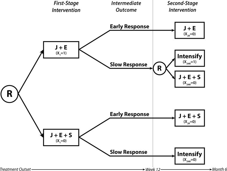
SMART design from an autism trial [19] including 3 embedded DTRs. The R inside a circle denotes randomization; J denotes joint attention and joint engagement; E denotes enhanced milieu teaching; S denotes speech generating device; X1 denotes coding for first-stage intervention; X2R and X2NR denote coding for second-stage intervention for responders and non-responders, respectively.
In general, we write DTRs as triplets of the form (x1, x2R, x2NR), where x1 is the recommended first-stage intervention, x2R the recommended second-stage intervention for responders, and x2NR the recommended second-stage intervention for non-responders. The three embedded DTRs in Figure 1 are (J+E, J+E, Intensify), (J+E, J+E, J+E+S), and (J+E+S, J+E+S, Intensify).
2.1. Common SMART designs
We present three of the most common two-stage SMART designs in Figure 2 and use dummy coding to denote the intervention options (likewise we could have used contrast or other coding). We consider only two-stage trials since, currently, most investigators developing DTRs are interested in implementing two-stage SMARTs. The designs shown only include two intervention options for randomization at the first and second stages. However, the methods presented easily extend to SMARTs with three or more stages or where individuals are randomized between three or more interventions options at any stage. The three SMART designs differ by the number of embedded DTRs since second-stage randomization can depend on first-stage intervention and tailoring variable status. We denote the tailoring variable as a binary measure of response (not necessarily the same binary overall outcome at the end of the study) and refer to those who have the potential of re-randomization as responders or non-responders. The tailoring variable, however, could be defined differently as any dichotomous intermediate outcome (e.g. adherence vs. non-adherence; for examples from SMARTs in the field, see [24]).
Figure 2.

Three common SMART designs. Design I includes 8 embedded DTRs, design II includes 4 embedded DTRs, and design III includes 3 embedded DTRs. The R inside a circle denotes randomization; X1 denotes coding for first-stage intervention; X2R and X2NR denote coding for second-stage intervention for responders and non-responders, respectively. The tailoring variable is trial-specific with intermediate outcome denoted here by response and non-response.
Design I, shown in Figure 2, is a general design where all individuals are re-randomized, but specific second-stage intervention can depend on the first-stage intervention and/or response status. This design has been used in practice investigating the development of DTRs in the treatment of drug dependent pregnant women [18] and alcohol dependence [38]. Within this general SMART design, there are eight embedded DTRs. For example, one such DTR is to first treat with x1 = 1 followed by x2R = 1 if response and x2NR = 1 if no response (DTR denoted by (1,1,1)). A person who follows any particular pathway in this SMART design is consistent with two embedded DTRs. For example, a non-responder to x1 = 1 who received x2NR = 0 could follow either of the following DTRs: (1,1,0) or (1,0,0).
In another common SMART design, design II in Figure 2, randomization in the second stage depends on the intermediate outcome. In this figure, only non-responders are re-randomized. One may also consider the design where responders and non-responders are switched such that only responders are re-randomized. This may occur in trials, for example in oncology, where the second-stage intervention is a maintenance intervention and there are no further options for those who do not respond to the first-stage intervention. Examples of design II in practice include investigations of the treatment of ADHD [40], acute myelogenous leukemia [45, 46], small-cell lung cancer [48], neuroblastoma [29, 30], diffuse large cell lymphoma [15], multiple myeloma [28], and metastatic malignant melanoma [5]. There are four DTRs embedded in this design: (1,0,1), (1,0,0), (0,0,1), and (0,0,0). In this trial, responders to the first-stage intervention are consistent with two DTRs. This aspect of the design must be accounted for in the analysis of the trial.
SMART design III in Figure 2 is a general depiction of the autism trial [19]. In this design, only one set of participants are re-randomized, depending on first-stage intervention and response status. This design may be appropriate when randomization is not ethical or feasible depending on first-stage intervention. In the autism trial, the investigators felt that it was inappropriate to take away the speech generating device from children who had received it, and that the only suitable second-stage intervention option for slow responders which used the device was intensified first-stage intervention. This SMART contains three embedded DTRs, denoted (1,0,1), (1,0,0), and (0,0,0). Another example of this design is a cluster randomized SMART investigating adaptive implementation strategies to improve mental health outcomes among adults with mood disorders [20].
3. Analysis of SMARTs with binary endpoint
3.1. Modeling
We briefly review logistic regression methods for comparing two DTRs and the implementation of the models for the analysis of SMART data with a binary endpoint. We point the readers to the analysis of SMART data with a continuous outcome for more details [34]. For simplicity, we focus on saturated logistic regression models for each of the three SMART designs presented earlier.
Let Y be a binary outcome indicating success (Y = 1) or failure (Y = 0). Let p = p(x1, x2R, x2NR) denote the probability of success (Y = 1) at the end of the intervention had all participants followed the DTR denoted by (x1, x2R, x2NR). We denote the vector of the proportions of success for all DTRs as p.
We note that baseline covariates may be added to the saturated logistic models, but any covariates measured after the initial randomization should not be included as they can lead to bias [42] (see [34] for more details). Baseline covariates may be included in the models or used instead in the estimation of weights (time-varying covariates may also be used to estimate weights) for the DTR groups [7]. We do not include them here for simplicity and since we do not use these variables in the derivation of the sample size equation.
For SMART design I, the saturated logistic model can be specified as:
| (1) |
where the β is a vector of unknown parameters and logit [24]. For example, based on this logistic model, we may be interested in comparing the DTRs from Figure 2 (1,1,1) versus (0,1,1). For this comparison, the difference in log-odds between the two DTRs reduces to the linear combination of regression coefficients: β1 + β4 + β5 + β7. Similarly, other contrasts may be formed to compare other pairs of DTRs.
For SMART design II, the logistic model can be written as:
| (2) |
and for SMART design III, the logistic model is:
| (3) |
These models differ from previously proposed regression models for data from SMARTs by Bembom and van der Laan [6, 7] by including an interaction term between first- and second-stage intervention indicators and the estimation of standard errors (see Section 3.2). The interaction between first- and second-stage interventions allows for non-additive intervention effects including the possibility of synergistic (or antagonistic) effects between the first- and second-stage interventions.
3.2. Review of Estimation
In most cases, estimation methods for comparing DTRs with SMART data differ from that with data from a standard RCT due to sequential randomizations. Thus, we briefly review an estimation procedure to analyze data from a SMART with a binary outcome using logistic regression and standard software [34, 37]. The method involves weighting and, in order to implement it with standard software, a replicating data step. We assume consistency and sequential ignorability which we have by SMART design.
The ‘weighted and replicated’ estimation method weights and replicates observations to account for the restricted randomization by design. Many SMART designs include restricted randomization by only randomizing some of the trial participants to specific intervention options (e.g., in design II only non-responders are re-randomized to receive intensified or additional therapy), unequal randomization between interventions at the first and/or second stage, or randomization to different numbers of interventions (for example, non-responders could receive one of three possible interventions, whereas responders could receive one of two possible interventions) [34]. When any of these three scenarios occur, there is under- or over-representation of certain groups of individuals due to the design of the trial. To account for this, inverse-probability-of-treatment weighting is used [16]. Each observation is weighted inversely proportional to its probability of receiving its own DTR. The weights are known; they are obtained from the assigned randomization probability to the first- and second-stage intervention options.
For the most commonly used and presented designs, weights are not needed for design I if all individuals are randomized at the first- and second-stages with equal probability, but are needed for designs II and III regardless of equal randomization, since not all participants are randomized at the second-stage. For example, for design III, only the non-responders to intervention X1 = 1 are randomized twice, so their weight is 1/(0.5*0.5)=4. Since the responders to X1 = 1 and all those who received X1 = 0 were only randomized once, their weight is 1/0.5=2. We note that we have used the known randomization probabilities as the weights in the estimation process, but weights may be estimated using trial data and baseline covariates. This leads to greater efficiency [42].
After observations are weighted, the observations that are consistent with more than one DTR are replicated in order to estimate and compare the effects of the DTRs simultaneously using standard software [34]. Data from a SMART includes the specific intervention path (sequence) followed by each participant. Replication modifies the data to include each DTR followed by the participant. For example, in design III, only the responders to intervention X1 = 1 are replicated since they are consistent with two DTRs; we set X2NR=1 for one observation and X2NR=0 for the other.
Once the weights and new data structure with replication have been appropriately applied, estimation may be done using any standard software package that incorporates generalized estimating equations (GEE) estimators (e.g. SAS, STATA, SPSS, R). Although weights are known from the randomization probabilities, the weights assigned to each individual depends on intermediate response status. The observed rate of response may vary from trial to trial, so the robust asymptotic variance estimators are used to account for this sample-to-sample variation in the distribution of weights and for the replication of individuals in the new data structure [34]. More details on the estimating equations are given in Appendix A.
3.3. Hypothesis Testing
There are several different metrics and tests to compare groups when the data is binary (e.g. differences in proportions, test of ratios or odds ratios, score or wald tests). Assuming researchers will use the logistic regression ‘weighted and replicated’ estimation procedure presented above to test hypotheses about DTRs of interest, we support the Wald test of a combination of coefficients from the model since it is commonly applied to test hypotheses.
For the Wald test, interest is in the odds ratio of the two DTRs defined by the odds of one DTR divided by the odds of the other DTR, where we denote the DTR used in the denominator as the reference DTR. Since our regression equations are in the log odds scale, the hypothesis test can be written as a difference in log odds of the two DTRs of interest. We denote c as a vector specifying the linear combination of regression coefficients indicating the difference in the log odds of the two DTRs of interest, such that the hypothesis test for comparing the log odds of two DTRs can be written as H0 : cTβ = 0 versus HA : cTβ ≠ 0.
For example, consider the analysis of a SMART with design III comparing DTRs denoted by (1,0,1) and (0,0,0) in Figure 2. The log odds for each group are β0 + β1 + β2 and β0, respectively, such that the hypothesis test is defined as above where c = (0, 1, 1).
To test this hypothesis, we can use the Wald test. Since a comparison of two DTRs will result in a one degree of freedom test, we present the Z-statistic. Thus, the test is specified as
where denotes the estimates of the regression coefficients and denotes the estimated covariance matrix of .
4. Sample Size
4.1. Sample Size Calculation
Once science has guided the specific SMART design of interest, a binary variable has been chosen as the primary outcome, and an analytic plan has been specified, often, the next step is to size the trial to have sufficient power to find an effect of interest. The sample size for any clinical trial is a balance between having enough participants to find a clinically and statistically significant effect, but not having so many participants that resources are wasted or many are exposed to a possibly suboptimal intervention. Just as in any trial, a SMART should be powered based on its primary objective. If stage-specific intervention questions (e.g. a comparison of first-stage interventions averaging over response and second-stage interventions) are of primary interest and embedded DTR development is secondary, SMARTs may be powered similar to a standard RCT [35]. If, however, a comparison of embedded DTRs (beginning with different interventions) is of primary interest, sample size calculations specific to a SMART must be considered.
We provide sample size formulae for the case where researchers are interested in a primary aim comparison of two DTRs that begin with different interventions. For example, the autism SMART could have been powered to find the difference between the DTR with the least aggressive interventions, (J+E, J+E, Intensify), versus the DTR with the most aggressive interventions, (J+E+S, J+E+S, Intensify). We present the sample size calculation as a modification to the standard sample size formula for logistic regression as detailed in [11, 12]. A more complete derivation of the sample size based on the Wald test statistic is provided in Appendix A.
In the derivation of the sample size formula, we make several assumptions. We assume that the variability of the outcome around the strategy log odds among responders and non-responders is no more than the variance of the strategy log odds [35] and a large enough sample size with success probability bounded away from 0 and 1 for the usual assumptions of the Wald test to hold. We present the sample size formula in general form in equation 4, where the probabilities of randomization can take any value at the first and second stage and the probabilities of response can differ between first-stage treatments.
Let α be the significance level of the hypothesis test, Z1 − α/2 is the standard normal 1 − α/2 percentile, and Zq is the qth quantile (the power of the study, typically 0.8 or 0.9). We present the sample size calculation using the expected proportions of the DTRs of interest, but one can elicit any of the other effect sizes (e.g. odds ratio, rate ratio or relative risk, phi coefficient) depending on the experience and comfort of the investigators and some additional information (e.g. the proportion of success for one DTR or for pathways that make up one DTR) and calculate the others (see Section 4.2). Further, the sample size is presented for the entire SMART.
The total sample size of a SMART comparing the proportions between two DTRs of interest can be written as:
| (4) |
where A and B depend on the design, p1 and p2 are the proportions of success of the DTRs of interest, and is the odds ratio (i.e. effect size) of two DTRs of interest. We can elicit the two proportions of interest or one proportion and the OR. Table 1 gives the values of A and B by design and pairwise DTR comparison of interest. For example, for design III, if interest is in comparing DTR (1, 0, 1) versus (0,0,0), and .
Table 1.
Values A and B in the sample size calculation comparing two embedded DTRs from a SMART.
| Conservative Estimate of A or B | |||||||
|---|---|---|---|---|---|---|---|
| Design | DTR | A or B | rk = 0, k = 0, 1 | rk = 1, k = 0, 1 | |||
| I | (1,1,1) |
|
|
|
|||
| (1,1,0) |
|
|
|
||||
| (1,0,1) |
|
|
|
||||
| (1,0,0) |
|
|
|
||||
| (0,1,1) |
|
|
|
||||
| (0,1,0) |
|
|
|
||||
| (0,0,1) |
|
|
|
||||
| (0,0,0) |
|
|
|
||||
| II | (1,0,1) |
|
|
||||
| (1,0,0) |
|
|
|||||
| (0,0,1) |
|
|
|||||
| (0,0,0) |
|
|
|||||
| III | (1,0,1) |
|
|
||||
| (1,0,0) |
|
|
|||||
| (0,0,0) |
|
|
|||||
π1 is the probability of randomization to X1 = 1; π2R|1 and π2R|0 are the probabilities of randomization to X2R = 1 given X1 = 1 and X1 = 0, respectively; π2NR|1 and π2NR|0 are the probabilities of randomization to X2NR = 1 given X1 = 1 and X1 = 0, respectively; and r1 and r0 indicate hypothesized response rates to first-stage interventions X1 = 1 and X1 = 0, respectively. Conservative estimates for design I depend on the DTRs of interest and the values of π2R|k, π2NR|k for k = 0, 1, such that in some situations rk = 1, k = 0, 1 gives the conservative estimate and in others rk = 0, k = 0, 1 gives the conservative estimate. For designs II and III, conservative estimates are all given by rk = 0, k = 0, 1.
A and B are given if estimation of several parameters can be elicited: probability of response to first-stage treatments (P(R = 1|X1 = 1) = r1, P(R = 1|X1 = 0) = r0), probability of randomization to first-stage treatment (P(X1 = 1) = π1), and probability of randomization to second-stage treatments (P(X2R = 1|X1 = 1, R = 1) = π2R|1, P(X2NR = 1|X1 = 1, R = 0) = π2NR|1, P(X2R = 1|X1 = 0, R = 1) = π2R|0, P(X2NR = 1|X1 = 0, R = 0) = π2NR|0).
The probabilities of randomization will be known prior to the start of the SMART and thus can be provided, but the probabilities of response may be difficult to for investigators to have a good guess prior to the trial. Investigators may choose to provide a grid of potential sample sizes or power for differing response values. Alternatively, if the probability of non-response is high such that a substantial proportion of participants will be re-randomized in second stage, but investigators cannot provide a guess for the value of r, a conservative value may be used for the sample size. For design I, if π2R|k = π2NR|k = 0.5, k = 0, 1, the values of rk, k = 0, 1 are unnecessary and the conservative estimates of sample size are equal to the non-conservative estimates. If, however, in design I there is unequal randomization at the second-stage for responders or non-responders, a guess of rk, k = 0, 1 is necessary or a conservative value must be calculated. For design I, the conservative value of r depends on the DTRs of interest and the values of π2R|k and π2NR|k, for k = 0, 1. For example, if π2R|k = π2NR|k < 0.5, k = 0, 1, then rk = 1, k = 0, 1 provides conservative estimates of sample size when DTRs (1,1,0) or (0,1,0) are of interest, but rk = 0 provides conservative estimates when DTRs (1,0,1) or (0,0,1) are of interest. Our applet is preprogrammed to select the correct conservative value. Otherwise, one can calculate both A or B for rk = 0 and rk = 1 for k = 0, 1 and choose the larger value for implementation. Thus, for design I, conservative values overestimate the sample size only when there is unequal randomization to second-stage treatments (on the order of a 20% sample size increase). For designs II and III, conservative estimates of the sample sizes all assume the probability of response is 0. These estimates are the most conservative for design II (on the order of 15-30% increase in sample size) and lesser so, but still conservative for design III (on the order of 10-13% increase in sample size). Thus, a better guess of the probability of response from previous studies or pilot work can lead to sample size savings, particularly for cases of unequal randomization probabilities and designs II and III.
For the special case where the probability of randomization is always 50%, there are two treatment options at every randomization, and the probability of response to both first-stage treatments is equal (i.e. P(R = 1|X1 = 1) = P(R = 1|X1 = 0) = r), the sample size formula simplifies to the standard sample size formula for a 2-arm comparison ([8]) multiplied by a SMART-specific design effect (DE) as follows:
| (5) |
where is the odds ratio (i.e. effect size) of two DTRs of interest and DE denotes a design effect which is specific to the implemented trial design. Table 2 presents the specific design effects associated with the three common SMART designs shown in Figure 2 where r denotes the estimate of the probability of response to first-stage intervention, if provided, which is assumed to be equal among first-stage interventions. If the investigator does not believe response probabilities to the firststage interventions are equal, but cannot provide a good estimate for both to use equation 4, the lowest probability of response between the first-stage interventions should be used to yield conservative estimates. If the probability of response cannot be estimated at all, a conservative sample size calculation is given when r=0 [35].
Table 2.
The design effect included in the sample size calculation comparing two proportions of embedded DTRs from a SMART when all of the probabilities of randomization are 50%, there are only two treatment options at every randomization, and the probability of response to first-stage treatments is equal.
| Design | Design Effect DE | |||
|---|---|---|---|---|
| Probability of Response provided | Conservative Estimate | |||
| I | 2 | 2 | ||
| II | 2 − r | 2 | ||
| III |
|
|
||
r indicates a hypothesized response rate to first-stage interventions.
4.2. Elicitation of Sample Size Parameters
The information needed to calculate this sample size may be elicited from investigators in many different ways. For example, the investigators may supply p1 and p2 and the various probabilities of randomization (π1, π2R|1, π2NR|1, π2R|0, π2NR|0), and the probabilities of response (r1, r0) for the direct calculation of the sample size using equation 4. It may be difficult to obtain the probabilities of success for the DTRs (i.e., p1 and p2), so that eliciting the probabilities of success of the intervention pathways (i.e. (x1, x2R) and (x1, x2NR)) may instead be more intuitive. Proportions of success for each pathway may be more readily available from previous studies or observational data.
For design III, this would entail providing the expected probability of the outcome for the subgroups who receive intervention x1 = 1, respond and receive intervention X2R = 0; receive X1 = 1, do not respond and receive X2NR = 1; receive X1 = 1, do not respond and receive X2NR = 0; receive X1 = 0, respond and receive X2R = 0; and receive X1 = 0, do not respond and receive X2NR = 0. In terms of the autism trial, if we were to calculate the sample size before the trial began, we would ask the researchers if they could estimate the probability of response to J+E (r1) and the proportion who would have high communication at 6 months for the following groups:
children who start with J+E, respond early and remain on J+E,
children who start with J+E, are slow to respond and receive intensified J+E at week 12,
children who start with J+E, are slow to respond and add a speech generating device to J+E at week 12,
children who start with J+E+S, respond early and remain on J+E+S, and
children who start with J+E+S, are slow to respond and receive intensified J+E+S at week 12.
The probability of the outcome may be constructed for each DTR from these estimates and the estimated probability of response to first-stage intervention (or a conservative estimate of no response, r=0).
Once the effect size, power, and significance of the test is given, these calculations can be coded using standard software modified by the design effect. For ease of implementation with details about SMART design and the calculation, we have created a user-friendly applet (found at http://sites.google.com/a/umich.edu/kidwell/) that requests the inputs of interest and outputs sample size or power for a SMART with design I through III or allows the investigator to create their own SMART design (i.e., allowing additional treatment arms and variations of SMART designs). In this calculator, we give a choice of the initial information given—odds ratio, probabilities of DTRs or probabilities of pathways—for ease of use. The applet has also been coded to produce sample size calculations for comparing two DTRs with continuous outcomes based on results from Oetting et al. [35].
5. Evaluation of Sample Size Calculation using Simulations
5.1. Simulation Results of Empirical Power
In this section we present results from simulations to test our sample size calculation using the presented Wald test. We calculated sample size to compare the following two DTRs in designs I, II and III: (1,0,1) and (0,0,0). Power was set to 0.8 and type I error to 0.05 using given weights based on equal randomization to interventions at the first and second stages. We specified different values for the proportion of success for DTRs 1 and 2 to evaluate the sample size needed to find moderate effect sizes: odds ratios of 2 and 2.5. We set the probability of response to the first-stage treatments equal and also explored if they differed. Empirical power was estimated by the proportion of times out of the 5,000 simulations that the null hypothesis was correctly rejected. We estimated the sample size and power as if the researchers could specify all of the parameters using Table 1 column 3 (i.e. the various probabilities of randomization and response) and also if response could not be estimated so that the conservative estimates would be given using Table 1 columns 4–5.
From Table 3, sample sizes increase when the odds ratio of the two DTRs of interest is closer to 1.0 and the probability of response is closer to 0 as expected. Power for the Wald test is generally equal to the expected power of 0.80 and may be slightly conservative for large effect sizes when all of the trial parameters are specified. For design I, the conservative estimates were equal to the fully specified estimates due to the balance of the design and equal probabilities of randomization to first- and second-stage treatments. For design II, the conservative estimates were that of design I and considerably overestimated the sample size. The conservative sample size also overestimated the number needed for design III, but on the order of 5% increase in power.
Table 3.
Empirical power of the sample size calculation for a two-sided test at 0.05 level with desired power of 80% for odds ratios of 2 and 2.5.
| Design | p1 | p2 | OR | r1 | r0 | All specified | Conservative | ||
|---|---|---|---|---|---|---|---|---|---|
| N | Power | N | Power | ||||||
| I | 0.54 | 0.70 | 2.0 | 0.30 | 0.30 | 574 | 0.805 | 574 | 0.805 |
| 0.41 | 0.64 | 2.5 | 0.30 | 0.60 | 317 | 0.807 | 317 | 0.807 | |
| 0.29 | 0.44 | 2.0 | 0.30 | 0.30 | 583 | 0.812 | 583 | 0.812 | |
| 0.29 | 0.50 | 2.5 | 0.30 | 0.60 | 335 | 0.808 | 335 | 0.808 | |
| II | 0.54 | 0.70 | 2.0 | 0.30 | 0.30 | 488 | 0.814 | 574 | 0.868 |
| 0.41 | 0.64 | 2.5 | 0.30 | 0.60 | 246 | 0.812 | 317 | 0.897 | |
| 0.29 | 0.44 | 2.0 | 0.30 | 0.30 | 496 | 0.810 | 583 | 0.867 | |
| 0.29 | 0.50 | 2.5 | 0.30 | 0.60 | 262 | 0.800 | 335 | 0.902 | |
| III | 0.54 | 0.70 | 2.0 | 0.30 | 0.30 | 379 | 0.815 | 418 | 0.850 |
| 0.41 | 0.64 | 2.5 | 0.30 | 0.60 | 213 | 0.804 | 236 | 0.842 | |
| 0.29 | 0.44 | 2.0 | 0.30 | 0.30 | 403 | 0.805 | 451 | 0.856 | |
| 0.29 | 0.50 | 2.5 | 0.30 | 0.60 | 232 | 0.816 | 260 | 0.853 | |
p1 denotes the proportion of success of one (reference) DTR (1,0,1), p2 denotes the proportion of success for the other DTR (0,0,0), N is the total sample size, r1 and r0 (relevant only for the all specified sample size calculation) is the probability of response to first-stage treatment X1 = 1 and X1=0, respectively. We have assumed equal probability of randomization at stages 1 and 2. ‘All specified’ and ’Conservative’ designate using A and B in Table 1 columns 3 and 4, respectively.
From Table 4, unequal randomization at the first-stage and in both stages increased the necessary sample size compared to that from Table 3, considering other trial parameters equal. The empirical power remained around expected for all designs, but was slightly increased in designs II and III. The conservative estimates changed for design I when both first and second-stage randomization probabilities changed and increased substantially for designs II and III similar to results from Table 3. Results considering other unequal randomization schemes were similar.
Table 4.
Empirical power of the sample size calculation for a two-sided test at 0.05 level with desired power of 80% for odds ratios of 2 (p1 =0.54, p2=0.70) and 2.5 (p1=0.41, p2=0.64).
| All specified | Conservative | ||||||||
|---|---|---|---|---|---|---|---|---|---|
| Design | OR | r1 | r0 | π2R|1 | π2NR|1 | N | Power | N | Power |
| I | 2.0 | 0.3 | 0.3 | 0.50 | 0.50 | 668 | 0.809 | 668 | 0.809 |
| 2.5 | 0.3 | 0.6 | 0.50 | 0.50 | 362 | 0.808 | 362 | 0.808 | |
| 2.0 | 0.3 | 0.3 | 0.67 | 0.67 | 641 | 0.808 | 769 | 0.863 | |
| 2.5 | 0.3 | 0.6 | 0.67 | 0.67 | 346 | 0.805 | 421 | 0.878 | |
| II | 2.0 | 0.3 | 0.3 | – | 0.50 | 568 | 0.819 | 668 | 0.891 |
| 2.5 | 0.3 | 0.6 | – | 0.50 | 271 | 0.823 | 362 | 0.905 | |
| 2.0 | 0.3 | 0.3 | – | 0.67 | 525 | 0.814 | 618 | 0.872 | |
| 2.5 | 0.3 | 0.6 | – | 0.67 | 246 | 0.816 | 333 | 0.912 | |
| III | 2.0 | 0.3 | 0.3 | – | 0.50 | 403 | 0.798 | 432 | 0.840 |
| 2.5 | 0.3 | 0.6 | – | 0.50 | 222 | 0.821 | 239 | 0.835 | |
| 2.0 | 0.3 | 0.3 | – | 0.67 | 368 | 0.813 | 382 | 0.825 | |
| 2.5 | 0.3 | 0.6 | – | 0.67 | 201 | 0.816 | 210 | 0.826 | |
N is the total sample size, r1 and r0 (relevant only for the all specified sample size calculation) is the probability of response to first-stage treatment X1 = 1 and X1=0, respectively, π2R|1 is the probability of randomization to second-stage intervention for responders to X1 = 1 and π2NR|1 is the probability of randomization for non-responders to X1 = 1. Randomization to first-stage intervention is unequal such that π1 =0.67 or about two thirds of participants are randomized to X1 = 1. All other randomization probabilities (π2R|0, π2NR|0) were equal and set to 0.5 if applicable to the design. All specified and Conservative designate using A and B in Table 1 columns 3 and 4 or 5, respectively.
We caution users against using this sample size calculation in some settings (which are unlikely to occur) and are due to the aberrant behavior of the Wald statistic for large effect sizes [1]. Unstable results may occur with a large effect size (i.e a large odds ratio) since the resulting sample size will be low. This is particularly a problem if estimations are not accurate in terms of the probability of response to the firststage intervention (or if there is drop out), since this may result in the number of people in each treatment pathway being too small to allow for the estimation of DTR effects. We believe that in most scientific settings, however, effect sizes of interest will be relatively modest so that the sample size calculator is relevant to many trials and generally robust to realistic assumptions.
6. Discussion
This manuscript reviews a ‘weighted and replicated’ estimation method of analysis. It also presents a sample size calculator for three common types of SMART designs where the primary objective is to compare two embedded DTRs (beginning with different treatments) on a binary outcome. Easy to use software to implement the sample size calculation and to guide investigators is available at http://sites.google.com/a/umich.edu/kidwell/ and sample R and SAS code for analysis of SMART data is given in the appendix. Since analysis can be executed using standard software and the sample size estimate is adapted from a standard Wald test, we hope that more investigators will view SMARTs as an approachable trial design and a possible addition to their trial toolkit to explore relevant intervention questions. This will enable the investigation of more tailored intervention sequences that are currently in use or that could be used in a trial setting and provide rigorous evidence for successful and realistic DTRs that enhance clinical practice.
Our sample size calculation differs from others which have recently been presented for continuous outcomes and extend to binary outcomes. First, our calculation differs from that of [39] because it allows for three types of two-stage SMART designs (as opposed to only design II and the online calculator version extends to other designs), and allows for any randomization allocations at stages 1 and 2 (as opposed to equal randomization to 2 treatments). Second, our sample size equation differs slightly from the one presented in [36]. The main calculation in [36] was for continuous outcomes but can extend to binary outcomes. The calculation by [36] was presented for various SMART designs (designs I, II and a three arm version of design II), but excluded design III, the design of the autism trial. Their calculation lacked easy-to-use software to implement the calculation for any design. In addition, our variance calculation comparing two embedded DTRs differs (and is somewhat simpler) and thus gives slightly different sample sizes. Further, our test is tied to the Wald test from ‘weighted and replicated’ regression so that standard software can be used.
Note that if the primary interest is in more than one pairwise comparison between DTRs, the proposed calculation and the corresponding applet can be used applying a Bonferroni (or one’s favorite multiple comparison) correction. All pairwise comparisons of interest with the correction can be computed and the largest sample size from these calculations would be chosen as the final sample size for the trial.
The sample size calculation given in equation 4 does not assume any particular number of treatments in each stage, but the specific A and B values given in Table A2 assumes only two treatments. A or B is given by depending on the DTR (x1, x2R, x2NR). Thus, the values of A and B can easily be extended to account for any number of treatments at any stage by introducing additional probabilities of response and randomization. The sample size calculation can also be extended to more than two stages, but we do not present additional details here due to the added complexity of defining the DTRs of interest and lack of three-or-more-stage SMARTs in the field.
The sample size calculation presented here does not allow for additional information concerning the relationship between a baseline covariate and the outcome; this is an area for future work. Further, we have noted the potential problems using the Wald test and, thus, small sample size corrections for the ‘weighted and replicated’ model and subsequent sample size calculations are also a future research endeavor.
Acknowledgments
Funding
The development of this article was funded by the following grants: ME-1507-31108, P50DA039838, R01DA039901, R01HD073975, R03MH09795401, and 5T32CA08365412.
All statements in this presentation, including its findings and conclusions are solely those of the authors and do not necessarily represent the views of the PCORI, its Board of Governors, or Methodology Committee.
APPENDIX A. Derivation of Sample Size Formula
We derive the sample size formula for a SMART design with a binary outcome and the goal of comparing two embedded DTRs beginning with different initial treatments using logistic regression and the Wald test. We have modified results from Oetting [35] and Demidenko [11, 12] to the setting of a SMART with estimation from generalized estimating equations with a binary outcome.
Consider a two-stage SMART design and suppose we are interested in sizing the trial for a pairwise comparison of two embedded DTRs, each with a different initial intervention. We continue using notation established in Sections 3 and 4 where x1 is an indicator of the first-stage intervention, x2R is an indicator of second-stage intervention for responders, and x2N R is an indicator of second-stage intervention for non-responders. We write DTRs in the form (x1, x2R, x2N R)·
First, we present the estimating equations such that solves the following equations:
| (A1) |
where I {subject i has data consistent with (x1, x2R, x2N R)}=1 if subject i has data consistent with DTR (x1, x2R, x2N R) and 0 otherwise, pi(x1, x2R, x2N R) is design dependent and defined as in Section 3.1 and Wi denotes the inverse-probability-of-treatment weights that are a function of X1, X2R, X2NR and R (an indicator of response).
In large samples, has a mean zero normal distribution with variable covariance matrix
and pi (x1, x2R, x2N R).
Let denote the variance of . In practice, we estimate by replacing the expectations in D and M with their empirical means and replacing β with . Let denote the so-called ‘plug-in’ estimate of . For additional details, see [34, 43].
Consider any of the logistic models presented in Section 3.1. We wish to test the null hypothesis H0: cTβ = 0 versus the alternative hypothesis HA: cTβ ≠ 0, where c is a vector indicating a linear combination of the difference in coefficients identifying the two DTRs of interest. For sample size purposes, we assume that under the alternative, cTβ = log(OR), where OR is the hypothesized odds ratio between the two DTRs of interest. As stated in Section 3.3 to test this null hypothesis versus the alternative that the two DTRs have different outcomes, we use the Wald test with 1 degree of freedom which can be written as the following Z-test:
To find the required sample size, n, for a two-sided test with type I error α and power q, we solve the following equation
for n where z1−α/2 is the standard normal (1 − α/2)th quantile.
Without loss of generality, letting the odds ratio of the two DTRs of interest, OR, be greater than 1, P{Z < −z1−α/2|cTβ = log(OR)} is negligible. So, P{Z > z1−α/2|cTβ = log(OR)} is equal to
By Slutsky’s theorem, we have well approximates for large n and we know that follows a standard normal distribution in large samples. Thus, we have
| (A2) |
Solving for n in equation A2, we have:
The final step is to express cD−1 MD−1c as a function of known or easily elicited quantities. To do this, we assume: for R = 0 and R = 1 (i.e. the variability of the outcome around the DTR log odds among responders and non-responders is no more than the variance of the DTR log odds), it is possible to show that
where i and B are given in Table 1 and p1 and p2 are the proportion of participants with Y = 1 at the end of the trial for the two DTRs of interest.
Hence, our sample size equation is
APPENDIX B. Sample Code for Implementing the ‘Weighted-and-Replicated’ Estimator in SAS and R using the Autism SMART Study (Design III) as an Example
The data should be in a format such that each individual is a row and columns include information about each individual. Columns should include individual ID, baseline covariates, first-stage intervention indicator (using format of 1 and 0), tailoring variable indicator (example, response or not), any other intermediate covariates, second-stage intervention indicator (using format of 1 and 0 for interventions) and overall outcome (0 or 1). In the sections below, we denote the tailoring variable indicator by R, first-stage intervention indicator by X1, and second-stage intervention indicator by X2.
B.1. In SAS
⋆Weight and replicate in data step;
DATA data;
 SET data;
 IF R = 1 and X1 = 1 THEN DO;
  ob = 1; X2 = 0; weight = 2; OUTPUT;
  ob = 2; X2 = 1; weight = 2; OUTPUT;
 END;
 ELSE IF R = 0 and X1 = 1 THEN DO;
  ob = 1; weight = 4; OUTPUT;
 END;
 ELSE IF X1 = 0 THEN DO;
  ob = 1; weight = 2; OUTPUT;
 END;
RUN;
DATA data2;
 SET data;
 * Create indicators to differentate {J+E, J+E, INTENSIFY} vs.;
 * {J+E, J+E, J+E+S} vs. {J+E+S, J+E+S, INTENSIFY}.;
 * X1 helps differentiate X1 = 1, {J+E, J+E, INTENSIFY} and;
 * {J+E, J+E, J+E+S}, from X1 = 0, {J+E+S, J+E+S, INTENSIFY}.;
 * But we need to differentiate the two sequences with X1 = 1 using X2.;
 X1X2 = X1*X2;
 *X2 is missing for observations following {J+E+S, J+E+S, INTENSIFY},;
 * so we reset missingess to zero.;
 IF X1X2 =. THEN X1X2 = 0;
 * We can now differentiate between all embedded DTRs:;
 * {J+E, J+E, INTENSIFY} is X1 = 1 and X1X2 = 1 ;
 * {J+E, J+E, J+E+S} is X1 = 1 and X1X2 = 0 ;
 * {J+E+S, J+E+S, INTENSIFY} is X1 = 0 and X1X2 = 0 ;
RUN;
⋆Logistic regression with sandwich error and estimation of overall
success rate for each DTR;
PROC GENMOD data = data2;
 CLASS id;
 MODEL outcome = X1 X1X2 / dist=bin link=logit;
 SCWGT weight;
 REPEATED subject=id / type=ind;
 * These statements request the logit of the ;
 * probability of success under each DTR. ;
 ESTIMATE ’Logit(p) under {J+E, J+E, INTENSIFY}’ int 1 X1 1 X1X2 1;
 ESTIMATE ’Logit(p) under {J+E, J+E, J+E+S}’ int 1 X1 1 X1X2 0;
 ESTIMATE ’Logit(p) under {J+E+S, J+E+S, INTENSIFY}’ int 1 X1 0 X1X2 0;
 * These statements request pairwise comparisons of DTRs;
 ESTIMATE ’Diff: {J+E, J+E, J+E+S} - {J+E+S, J+E+S, INTENSIFY}’ int 0 X1 1 X1X2 0; RUN;
B.2. In R
We note that if unequal randomization will be implemented for either the first or second stage, the R package geeglm may give an error due to non-integer weights. The package does estimate correctly, but to avoid the error, one can use the package survey with function svyglm.
#Libraries needed
library(geepack) #Required for geeglm function library(doBy) #Required for esticon function
library(aod) #Required for wald.test function
#Weight and Recycle
colnames(data) <- c(“X1”, “R”, “X2”, “Y”, “id”)
data$weight[R == 1] <- 2
data$weight [X1 == 1 & R == 0] <- 4
data$weight [X1 == 0 & R == 0] <- 2
data$toRecycle <- rep(0, dim(data)[1])
data$toRecycle[X1==1 & R==1] <- 1
numNoRecycle <- dim(data[data$toRecycle == 0,])[1]
dataNoRecycle <- cbind(data[data$toRecycle == 0,],
 seq(1, numNotRecycled, by=1)) dataRecycle1 <- data[data$R == 1,]
dataRecycle1$X2 <- 1
numRecycle <- dim(dataRecycle1) [1]
dataRecyclel <- cbind(dataRecycle1,
seq(numNoRecycle + 1, numNoRecycle + numRecycle)) dataRecycle2 <- data[data$toRecycle == 1, ]
dataRecycle2$X2 <- 0
dataRecycle2 <- cbind(dataRecycle2,
seq(numNoRecycle + 1, numNoRecycle + numRecycle))
dataRecycle <- rbind(dataNoRecycle, dataRecycle1, dataRecycle2)
colnames(dataRecycle) <- c(“X1”, “R”, “X2”, “Y”, “id”, “weight”,
“toRecycle”)
#Logistic regression with robust standard errors
sortDataRecycle <- dataRecycle[order(dataRecycle$id), ] glmDataRecycle <- geeglm(Y ~ X1 + X1*X2, id = id, weights = weight,
family = binomial(“logit”), corstr = “independence”, data = sortDataRecycle)
#Wald tests for pairwise comparisons
pairACDvsBFG.wald.chisq <- wald.test(b = coef(glmDataRecycle),
Sigma = vcov(glmDataRecycle),
L = cbind(0, 1, 1))
#Estimation of overall success rate for DTRs of interest
pACD <- exp(esticon(glmDataRecycle, c(1, 1, 1))$Estimate) /
(1 + exp(esticon(glmDataRecycle, c(1, 1, 1))$Estimate)) pBFG <- exp(esticon(glmDataRecycle, c(1, 0, 0))$Estimate) /
(1 + exp(esticon(glmDataRecycle, c(1, 0, 0))$Estimate))
APPENDIX C. Autism Trial Data Analysis
Here, we present the results using the ‘weighted and replicated’ estimation procedure and standard software for the autism SMART study [19]. In this trial, 61 minimally verbal children with autism spectrum disorder between the ages of 5 and 8 were enrolled following the design in Figure 1. For more details about this particular study see [3, 19, 26]. For our illustration, interest is in comparing the proportion of children who achieve a successful level of spoken communication between the three DTRs. The binary outcome is defined as having 40 or greater socially communicative utterances (success) versus fewer than 40 at week 24 of the study. Below, we report estimates of the proportions for each DTR as well as pairwise comparisons between the three DTRs. A sequential type of multiple imputation algorithm was used to replace missing values in the dataset (see [44]).
We estimate the β’s shown in the model in Equation 3, which represents a marginal model with no baseline covariates. For the weights, the slow responders who received J+E are given a weight of 4 and all others are given a weight of 2. Only the early responders to J+E are replicated. Code similar to that used for analysis appears in Appendix B. The results from the model are shown in Table A1. From this model, the proportion of success is estimated to be approximately 30% if all children were to follow the DTR given by (J+E, J+E, Intensify), 39% if all children were to follow the DTRs given by (J+E, J+E, J+E+S), and 75% if all children were to follow the DTR given by (J+E+S, J+E+S, Intensify). Thus, we see in Table A2 which provides odds ratios for the pairwise comparisons, that there are significantly higher odds of success or higher levels of communication for the DTR that begins with J+E+S compared to the DTRs that begin with J+E. There was no significant difference between the DTRs that both began with J+E, so that adding S or intensifying J+E did not result in significantly different proportions of success for slow responding children.
Table A1.
Results (parameter estimates) for ‘weighted and replicated’ regression of the autism SMART. SE denotes standard error. X1 denotes the initial intervention such that X1 = 1 denotes J+E and x1 = 0 denotes J+E+S; X2 denotes the second-stage intervention for non-responders such that x2 = 1 denotes intensify and x2 = 0 denotes adding the speech generating device.
| Parameter | Estimate | Robust SE | 95% Confidence Limits | P-value |
|---|---|---|---|---|
| Intercept | 1.10 | 0.34 | (0.43, 1.78) | <0.01 |
| X1 | −1.54 | 0.42 | (−2.36, −0.71) | <0.01 |
| x1x2N R | −0.42 | 0.45 | (−1.32, 0.47) | 0.35 |
Table A2.
The three pairwise comparisons of dynamic treatment regimens based on the ‘weighted and replicated’ regression of the autism SMART. DTR denotes dynamic treatment regimen, SE denotes standard error. The odds ratio is given as the odds of DTR 1 over the odds of DTR 2.
| DTR 1 | DTR 2 | Odds Ratio | 95% Confidence Limits | P-value |
|---|---|---|---|---|
| (J+E+S, J+E+S, Intensify) | (J+E, J+E, Intensify) | 7.10 | (2.44, 20.67) | <0.01 |
| (J+E+S, J+E+S, Intensify) | (J+E, J+E, J+E+S) | 4.64 | (2.03, 10.61) | <0.01 |
| (J+E, J+E, J+E+S) | (J+E, J+E, Intensify) | 1.53 | (0.63, 3.73) | 0.35 |
Footnotes
Disclosure statement
The authors do not have any conflicts of interest to disclose.
References
- 1.Agresti A. Categorical data analysis. John Wiley & Sons; 2013. [Google Scholar]
- 2.Almirall D, Compton SN, Gunlicks-Stoessel M, Duan N, Murphy SA. Designing a pilot sequential multiple assignment randomized trial for developing an adaptive treatment strategy. Statistics in Medicine. 2012;31:1887–1902. doi: 10.1002/sim.4512. [DOI] [PMC free article] [PubMed] [Google Scholar]
- 3.Almirall D, DiStefano C, Chang YC, Shire S, Kaiser A, Lu X, Nahum-Shani I, Landa R, Mathy P, Kasari C. Longitudinal effects of adaptive interventions with a speech-generating device in minimally verbal children with asd. Journal of Clinical Child and Adolescent Psychology. 2016;35:1595–1615. doi: 10.1080/15374416.2016.1138407. [DOI] [PMC free article] [PubMed] [Google Scholar]
- 4.Almirall D, Nahum-Shani I, Sherwood N, Murphy S. Introduction to smart designs for the development of adaptive interventions: with application to weight loss research. Translational Behavioral Medicine. 2014;4:260–274. doi: 10.1007/s13142-014-0265-0. http://dx.doi.org/10.1007/s13142-014-0265-0 Available at . . [DOI] [PMC free article] [PubMed] [Google Scholar]
- 5.Auyeung SF, Long Q, Royster EB, Murthy S, McNutt MD, Lawson D, Miller A, Manatunga A, Musselman DL. Sequential multiple-assignment randomized trial design of neurobehavioral treatment for patients with metastatic malignant melanoma undergoing high-dose interferon-alpha therapy. Clinical Trials. 2009;6:480–490. doi: 10.1177/1740774509344633. [DOI] [PMC free article] [PubMed] [Google Scholar]
- 6.Bembom O, van der Laan MJ. Statistical methods for analyzing sequentially randomized trials. Journal of the National Cancer Institute. 2007;99:1577–1582. doi: 10.1093/jnci/djm185. [DOI] [PMC free article] [PubMed] [Google Scholar]
- 7.Bembom O, van der Laan MJ. Analyzing sequentially randomized trials based on causal effect models for realistic individualized treatment rules. Statistics in Medicine. 2008;27:3689–3716. doi: 10.1002/sim.3268. [DOI] [PubMed] [Google Scholar]
- 8.Campbell M, Julious S, Altmani D. Estimating sample sizes for binary, ordered categorical, and continuous outcomes in two group comparisons. British Medical Journal. 1995;311:1145–1148. doi: 10.1136/bmj.311.7013.1145. [DOI] [PMC free article] [PubMed] [Google Scholar]
- 9.Collins L, Murphy S, Bierman K. A conceptual framework for adaptive preventive interventions. Prevention Science. 2004;5:185–196. doi: 10.1023/b:prev.0000037641.26017.00. [DOI] [PMC free article] [PubMed] [Google Scholar]
- 10.Dawson R, Lavori P. Sample size calculations for evaluating treatment policies in multi-stage designs. Clinical Trials. 2010;7:643–652. doi: 10.1177/1740774510376418. [DOI] [PMC free article] [PubMed] [Google Scholar]
- 11.Demidenko E. Sample size determination for logistic regression revisited. Statistics in Medicine. 2007;26:3385–3397. doi: 10.1002/sim.2771. http://dx.doi.org/10.1002/sim.2771 Available at . . [DOI] [PubMed] [Google Scholar]
- 12.Demidenko E. Sample size and optimal design for logistic regression with binary interaction. Statistics in Medicine. 2008;27:36–46. doi: 10.1002/sim.2980. [DOI] [PubMed] [Google Scholar]
- 13.Ertefaie A, Deng K, Wagner AT, Murphy SA. qlaci R package for using q-learning to construct adaptive interventions using data from a SMART (Version 1.0) University Park: The Methodology Center, Penn State; 2014. Available at methodology.psu.edu. [Google Scholar]
- 14.Feng W, Wahed AS. Supremum weighted log-rank test and sample size for comparing two-stage adaptive treatment strategies. Biometrika. 2008;95:695–707. [Google Scholar]
- 15.Habermann T, Weller E, Morrison V, Gascoyne R, Cassileth P, Cohn J, Dakhil S, Woda B, Fisher R, Peterson B, Horning S. Rituximab-CHOP verses CHOP alone or with maintenance Rituximab in older patients with diffuse large B-cell lymphoma. Journal of Clinical Oncology. 2006;24:3121–3127. doi: 10.1200/JCO.2005.05.1003. [DOI] [PubMed] [Google Scholar]
- 16.Hernán M, Brumback B, Robins J. Marginal structural models to estimate the causal effect of zidovudine on the survival of hiv-positive men. Epidemiology. 2000;11 doi: 10.1097/00001648-200009000-00012. [DOI] [PubMed] [Google Scholar]
- 17.Holloway ST, Laber EB, Linn KA, Zhang B, Davidian M, Tsiatis AA. Dyn-TxRegime: Methods for Estimating Dynamic Treatment Regimes. 2015 Available at https://CRAN.R-project.org/package=DynTxRegime, R package version 2.1.
- 18.Jones HE, OGrady KE, Tuten M. Reinforcement-based treatment improves the maternal treatment and neonatal outcomes of pregnant patients enrolled in comprehensive care treatment. The American Journal on Addictions. 2011;20:196–204. doi: 10.1111/j.1521-0391.2011.00119.x. http://dx.doi.org/10.1111/j.1521-0391.2011.00119.x Available at . . [DOI] [PMC free article] [PubMed] [Google Scholar]
- 19.Kasari C, Kaiser A, Goods K, Nietfeld J, Mathy P, Landa R, Murphy S, Almirall D. Communication interventions for minimally verbal children with autism: A sequential multiple assignment randomized trial. Journal of the American Academy of Child and Adolescent Psychiatry. 2014;53:635–646. doi: 10.1016/j.jaac.2014.01.019. Available at http://www.sciencedirect.com/science/article/pii/S0890856714001634. [DOI] [PMC free article] [PubMed] [Google Scholar]
- 20.Kilbourne A, Almirall D, Eisenberg D, Waxmonsky J, Goodrich D, Fortney J, Kircher J, Solberg L, Main M, Kyle J, Murphy S, Nord K, Thomas M. Protocol: Adaptive implementation of effective programs trial (adept): cluster randomized smart trial comparing a standard versus enhanced implementation strategy to improve outcomes of a mood disorders program. Implementation Science. 2014;9 doi: 10.1186/s13012-014-0132-x. [DOI] [PMC free article] [PubMed] [Google Scholar]
- 21.Lavori PW, Dawson R. A design for testing clinical strategies: Biased individually tailored within-subject randomization. Journal of the Royal Statistical Society A. 2000;163:29–38. [Google Scholar]
- 22.Lavori PW, Dawson R, J RA. Flexible treatment strategies in chronic disease: Clinical research implications. Biological Psychology. 2000;48:605–614. doi: 10.1016/s0006-3223(00)00946-x. [DOI] [PubMed] [Google Scholar]
- 23.Lavori PW, Dawson R, J RA. Dynamic treatment regimes: Practical design considerations. Clinical Trials. 2004;1:9–20. doi: 10.1191/1740774s04cn002oa. [DOI] [PubMed] [Google Scholar]
- 24.Lei H, Nahum-Shani I, Lynch K, Oslin D, Murphy SA. A “SMART” design for building individualized treatment sequences. Annual Review of Clinical Psychology. 2012;8:21–48. doi: 10.1146/annurev-clinpsy-032511-143152. [DOI] [PMC free article] [PubMed] [Google Scholar]
- 25.Li Z, Murphy SA. Sample size formulae for two-stage random trials with survival outcomes. Biometrika. 2011;98:503–518. doi: 10.1093/biomet/asr019. [DOI] [PMC free article] [PubMed] [Google Scholar]
- 26.Lu X, Nahum-Shani I, Kasari C, Oslin DW, Pelham WE, Fabiano G, Almirall D. Comparing dynamic treatment regimes using repeated-measures outcomes: modeling considerations in smart studies. Statistics in Medicine. 2016;45:442–456. doi: 10.1002/sim.6819. [DOI] [PMC free article] [PubMed] [Google Scholar]
- 27.Lynn KA, Laber EB, Stefanski LA. iqlearn: Interactive q-learning in r. Journal of Statistical Software. 2015;64:1–25. doi: 10.18637/jss.v064.i01. [DOI] [PMC free article] [PubMed] [Google Scholar]
- 28.Mateos MV, Orio A, Martínez-López J, Gutiérrez N, Teruel AI, de Paz R, García-Laraña J, Bengoechea E, Martín A, Mediavilla JD, Palomera L, de Arriba F, González Y, Hernández JM, Sureda A, Bello JL, Bargay J, Peñalver FJ, Ribera JM, Martín-Mateos ML, García-Sanz R, Cibeira MT, Ramos MLM, Vidriales MB, Paiva B, Montalbán MA, Lahuerta JJ, Bladé J, Miguel JFS. Bortezomib, melphalan, and prednisone versus bortezomib, thalidomide, and prednisone as induction therapy followed by maintenance treatment with bortezomib and thalidomide versus bortezomib and prednisone in elderly patients with untreated multiple myeloma: a randomised trial. The Lancet Oncology. 2010;11:934–941. doi: 10.1016/S1470-2045(10)70187-X. [DOI] [PubMed] [Google Scholar]
- 29.Matthay KK, Reynolds CP, Seeger RC, Shimada H, Adkins ES, Haas-Kogan D, Gerbing RB, London WB, Villablanca JG. Long-term results for children with high-risk neuroblastoma treated on a randomized trial of myeloablative therapy followed by 13-cis-retinoic acid: A children’s oncology group study. Journal of Clinical Oncology. 2009;27:1007–1013. doi: 10.1200/JCO.2007.13.8925. [DOI] [PMC free article] [PubMed] [Google Scholar]
- 30.Matthay KK, Villablanca JG, Seeger RC, Stram DO, Harris RE, Ramsay NK, Swift P, Shimada H, Black CT, Brodeur GM, Gerbing RB, Reynolds CP. Treatment of high-risk neuroblastoma with intensive chemotherapy, radiotherapy, autologous bone marrow transplantation, and 13-cis-retinoic acid, The New England. Journal of Medicine. 1999;341:1165–1173. doi: 10.1056/NEJM199910143411601. [DOI] [PubMed] [Google Scholar]
- 31.Murphy S. An experimental design for the development of adaptive treatment strategies. Statistics in Medicine. 2005;24:1455–1481. doi: 10.1002/sim.2022. [DOI] [PubMed] [Google Scholar]
- 32.Murphy S, Almirall D. Dynamic treatment regimens, in Encyclopedia of Medical Decision Making, M.W. Kattan, ed., Sage Publications, Thousand Oaks, CA. 2009:419–422. [Google Scholar]
- 33.Murphy SA, van der Laan MJ, Robins JM, CPPRG Marginal mean models for dynamic regimes. Journal of the American Statistical Association. 2001;96:1410–1423. doi: 10.1198/016214501753382327. [DOI] [PMC free article] [PubMed] [Google Scholar]
- 34.Nahum-Shani I, Qian M, Almirall D, Pelham W, Gnagy B, Fabiano G, Waxmonsky J, Yu J, Murphy S. Experimental design and primary data analysis for developing adaptive interventions. Psychological Methdos. 2012;17:457–477. doi: 10.1037/a0029372. [DOI] [PMC free article] [PubMed] [Google Scholar]
- 35.Oetting AI, Levy JA, Weiss RD, Murphy SA. Statistical methodology for a SMART design in the development of adaptive treatment strategies, in Causality and Psychopathology: Finding the Determinants of Disorders and their Cures, P. Shrout, K. Keyes, and K. Ornstein, eds., chap. 8, American Psychopathological Association, American Psychiatric Publishing, Inc., Arlington, VA. 2011:179–205. [Google Scholar]
- 36.Ogbagaber SB, Karp J, Wahed AS. Design of sequentially randomized trials for testing adaptive treatment strategies. Statistics in Medicine. 2016;35:840–858. doi: 10.1002/sim.6747. http://dx.doi.org/10.1002/sim.6747 Available at . [DOI] [PMC free article] [PubMed] [Google Scholar]
- 37.Orellana L, Rotnitzky A, Robins J. Dynamic regime marginal structural mean models for estimation of optimal dynamic treatment regimes, part i: Main content, International. Journal of Biostatistics. 2010;6 [PubMed] [Google Scholar]
- 38.Oslin D. Managing alcoholism in people who do not respond to naltrexone (EXTEND) 2005 http://clinicaltrials.gov/ct2/show/NCT00115037?term=oslin&rank=8.
- 39.Ghosh BCP, Cheung YK. (chap. Sample size calculations for clustered SMART designs, SIAM).ADAPTIVE TREATMENT STRATEGIES IN PRACTICE: PLANNING TRIALS AND ANALYZING DATA FOR PERSONALIZED MEDICINE. 2015;21:55–70. [Google Scholar]
- 40.Pelham W, Fabiano G. Evidence-based psychosocial treatments for attention-deficit/hyperactivity disorder. Journal of Clinical Child and Adolescent Psychology. 2008;37:184–214. doi: 10.1080/15374410701818681. [DOI] [PubMed] [Google Scholar]
- 41.Robins J. A new approach to causal inference in mortality studies with sustained exposure periods-application to control of the healthy worker survivor effect. Mathematical Modelling. 1986;7:1393–1512. [Google Scholar]
- 42.Robins JM. Association, causation, and marginal structural models. Synthese. 1999;121:151–179. [Google Scholar]
- 43.Scott PSA, Zeger L, Liang Kung-Yee. Models for longitudinal data: A generalized estimating equation approach. Biometrics. 1988;44:1049–1060. Available at http://www.jstor.org/stable/2531734. [PubMed] [Google Scholar]
- 44.Shortreed SM, Laber E, Stroup T Scott, Pineau J, Murphy SA. A multiple imputation strategy for sequential multiple assignment randomized trials. Statistics in Medicine. 2014;33:4202–4214. doi: 10.1002/sim.6223. http://dx.doi.org/10.1002/sim.6223 Available at . . [DOI] [PMC free article] [PubMed] [Google Scholar]
- 45.Stone RM, Berg DT, George SL, Dodge RK, Paciucci PA, Schulman PP, Lee EJ, Moore JO, Powell BL, Baer MR, Bloomfield CD, Schiffer CA. Postremission therapy in older patients with de novo acute myeloid leukemia: A randomized trial comparing mitoxantrone and intermediate-dose cytarabine with standard-dose cytarabine. Blood. 2001;98:548–53. doi: 10.1182/blood.v98.3.548. [DOI] [PubMed] [Google Scholar]
- 46.Stone RM, Berg DT, George SL, Dodge RK, Paciucci PA, Schulman PP, Lee EJ, Moore JO, Powell BL, Baer MR, Schiffer CA. Granulocyte-macrophage colony-stimulating factor after initial chemotherapy for elderly patients with primary acute myelogenous leukemia. New England Journal of Medicine. 1995;332:1671–1677. doi: 10.1056/NEJM199506223322503. [DOI] [PubMed] [Google Scholar]
- 47.Tang X, Melguizo M. DTR: An R package for estimation and comparison of survival outcomes of dynamic treatment regimes. Journal of Statistical Software. 2015;65:1–28. Available at http://www.jstatsoft.org/v65/i07/. [Google Scholar]
- 48.Tummarello D, Mari D, Graziano F, Isidori P, Cetto G, Pasini F, Santo A, Cellerino R. A randomized, controlled phase iii study of cyclophosphamide, doxorubicin, and vincristine with etoposide (CAV-E) or teniposide (CAV-T),followed by recombinant interferon-alpha maintenance therapy or observation, in small cell lung carcinoma patients with complete responses. Cancer. 1997;80:2222–2229. [PubMed] [Google Scholar]
- 49.Wallace M, Moodie E, Stephens D. Dynamic treatment regimen estimation via regression-based techniques: Introducing r package dtrreg. Journal of Statistical Software. 2016 accepted. [Google Scholar]
- 50.Xin J, Chakraborty B, Laber EB. qLearn: Estimation and inference for Q-learning. 2012 Available at https://CRAN.R-project.org/package=qLearn, R package version 1.0.
- 51.Zhang Y. listdtr: List-Based Rules for Dynamic Treatment Regimes. 2016 Available at https://CRAN.R-project.org/package=listdtr, R package version 1.0.