Prediction of Individualized Task Activation in Sensory Modality-Selective Frontal Cortex with ‘Connectome Fingerprinting’

Abstract

The human cerebral cortex is estimated to comprise 200-300 distinct functional regions per hemisphere. Identification of the precise anatomical location of an individual’s unique set of functional regions is a challenge for neuroscience that has broad scientific and clinical utility. Recent studies have demonstrated the existence of four interleaved regions in lateral frontal cortex (LFC) that are part of broader visual attention and auditory attention networks (Michalka et al., 2015; Noyce et al., 2017; Tobyne et al., 2017). Due to a large degree of inter-subject anatomical variability, identification of these regions depends critically on within-subject analyses. Here, we demonstrate that, for both sexes, an individual’s unique pattern of resting-state functional connectivity can accurately identify their specific pattern of visual- and auditory-selective working memory and attention task activation in lateral frontal cortex (LFC) using “connectome fingerprinting.” Building on prior techniques (Saygin, Osher et al., 2011; Osher et al., 2016; Tavor et al., 2016; Smittenaar et al., 2017; Wang et al., 2017; Parker Jones et al., 2017), we demonstrate here that connectome fingerprint predictions are far more accurate than group-average predictions and match the accuracy of within-subject task-based functional localization, while requiring less data. These findings are robust across brain parcellations and are improved with penalized regression methods. Because resting-state data can be easily and rapidly collected, these results have broad implications for both clinical and research investigations of frontal lobe function. Our findings also provide a set of recommendations for future research.

Graphical Abstract

1. Introduction

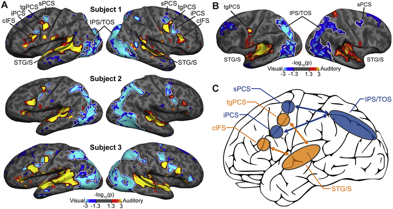
A central challenge for cognitive neuroscience is to determine the functional organization of human frontal cortex (e.g., Petrides and Pandya, 1995). Task-based fMRI approaches and other techniques have yielded considerable insights (e.g., Koechlin et al., 2003; Astafiev et al., 2003; Badre, 2008; Fedorenko et al., 2013; Sallet et al., 2013; Nee & D’Esposito, 2016), but many issues remain unresolved. Recent work has demonstrated that an individual’s unique pattern of functional or structural brain connectivity offers an alternative means to localize functional organization in individuals (Saygin, Osher et al., 2011; Osher et al., 2016; Tavor et al., 2016; Smittenaar et al., 2017; Wang et al., 2017; Parker Jones et al., 2017). Findings from our laboratory (Michalka et al., 2015; Tobyne et al., 2017) revealed multiple visual-selective and auditory-selective lateral frontal cortical areas that are nodes of separate whole-brain sensory modality-selective resting-state networks (Figure 1C). Here, we examine the utility of functional connectivity patterns in predicting the precise functional organization of sensory-selective regions within frontal cortex.

Fig. 1.

Sensory modality-selective attention regions in lateral frontal cortex, as described in Michalka et al., 2015; Noyce et al., 2017; Tobyne et al., 2017. (A) Three representative subjects from Michalka et al. (2015). Within LFC, two visual-selective regions, sPCS and iPCS, are interleaved with two auditory-selective regions, tgPCS and cIFS, bilaterally. The four regions (attend vision (cool colors) vs. attend audition (hot colors)) were observed bilaterally in 90% of individual subjects. (B) Group averaging of auditory vs. visual attention results from Michalka et al. (2015) obscured these regions, due to inter-subject anatomical variation. Group level (N = 9) analysis revealed only a single modality-selective LFC region in each hemisphere (tgPCS in left hemisphere; sPCS in right hemisphere). Only at the individual subject level were all four regions regularly identified (visualized here at p < 0.05, uncorrected). (C) Analysis of resting-state data reveals that the LFC regions form modality-specific functional networks with posterior visual (IPS/TOS) and posterior auditory (STG/S) attention regions. sPCS = superior precentral sulcus; tgPCS = transverse gyrus intersecting the precentral sulcus, iPCS = inferior precentral sulcus; cIFS = caudal inferior frontal sulcus, IPS/TPS = intraparietal sulcus/-transverse occipital sulcus, STG/S < superior temporal gyrus/sulcus.

Although sensory processing is typically considered to be restricted to posterior portions of the cerebral cortex, recent MRI studies demonstrate that specific influences of the visual and auditory sensory modalities extend to multiple regions of lateral frontal cortex (LFC) in humans (Michalka et al., 2015; Braga et al., 2017b; Mayer et al, 2017; Noyce et al., 2017; Tobyne et al., 2017). This focus on sensory modality selectivity complements a broad range of other approaches to understanding the functional organization of human LFC.

Multiple sensory-selective regions in LFC were observed by Michalka et al. (2015) by contrasting sustained attention to visual or auditory stimuli. This revealed two visual-selective regions (superior and inferior precentral sulcus; sPCS and iPCS) interleaved with two auditory-selective regions (transverse gyrus intersecting the precentral sulcus and caudal inferior frontal sulcus; tgPCS and cIFS), in each hemisphere of LFC (Figure 1A). Noyce et al. (2017) replicated these findings using a visual/auditory working memory (VAWM) paradigm. Accurate identification of these small, neighboring regions critically relies on individual subject analysis; while group-averaging methods obscure these regions (Figure 1B), all 8 regions were identified in 90% of individual subjects in both studies (Michalka et al., 2015; Noyce et al., 2017).

Efforts to parcellate human frontal lobe are constrained by the fact that distinct regions are small and their precise location varies across individuals. Functional MRI-based (fMRI) methods also face the challenge that frontal lobe activation requires performance of highly demanding cognitive tasks and acquisition of large amounts of functional data per subject, due to low signal amplitude. The approach of collecting exceedingly large amounts of data on individual subjects has proven successful in several recent fMRI investigations (Laumann et al., 2015; Braga et al., 2017a; Gordon et al., 2017). Despite the power and promise of these and other individual subject analyses (e.g. Michalka et al., 2013; Noyce et al., 2017), ‘deep sampling’ methods are cost prohibitive and their applicability appears limited to highly sophisticated subject pools, due to their significant cognitive and/or time demands. These approaches would be difficult or impossible to employ in clinical populations.

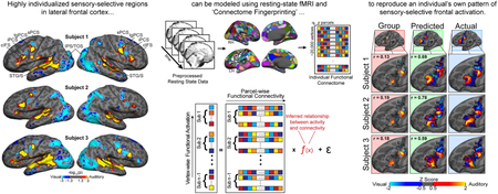
Here, we combine an individual subject approach with a penalized regression-based ‘connectome fingerprinting’ (CF) technique to predict the complex pattern of modality-selective attention areas in LFC. The use of connectivity-based techniques for predicting the functional architecture of the brain is in its infancy; therefore, we also examine the influence of algorithms, cortical parcellation methods, and data quality considerations on prediction accuracy. We show that CF predictions are capable of localizing an individual’s own unique pattern of auditory- and visual-selective functional recruitment using only their functional connectivity. We also present a series of recommendations for optimizing CF prediction techniques that should serve as a blueprint for future research. These methods require only a modest amount of resting-state functional MRI data and a modest subject pool size (N=9 in Michalka et al., 2015, N=14 in Noyce et al., 2015), and thus offer a widely applicable way to examine frontal lobe function in individual subjects.

2. Materials and Methods

2.1. Subject datasets

Two separate datasets from our laboratory were used for this work: 1) visual/auditory sustained attention (VASA) task fMRI (t-fMRI), resting-state fMRI (rs-fMRI) and high resolution structural MRI data from 9 subjects (mean age 27.66 ± 2.7, range 22-31, 5 females) previously published in Michalka et al., (2015), hereafter referred to as VASA9, and 2) visual/auditory working memory (VAWM) t-fMRI, rs-fMRI and anatomical data from 14 subjects (mean age 30 ± 2.8, range 25-35, 6 females) and previously published in Noyce et al. (2017); hereafter referred to as VAWM14. All subjects were healthy, right-handed, native English speakers and were recruited from the Boston University community. The Institutional Review Board of Boston University approved all experimental procedures. All subjects provided written informed consent in accordance with the guidelines set by Boston University.

Both the VASA9 and VAWM14 datasets were used in a series of connectome fingerprinting (CF) analyses investigating the capability of the technique to predict an individual’s unique pattern of task-driven functional recruitment within LFC. Several additional analyses were conducted with the VASA9 dataset to investigate optimal modeling procedures for such small, interleaved and variably located cortical regions. Seven subjects from the VASA9 dataset also participated in the VAWM14 dataset. Noyce et al. (2017) previously compared the VAWM task as a localizer for the VASA task and found that the contrast of auditory vs. visual working memory demands in the VAWM task recruits the same frontal regions as the contrast of sustained attention to auditory vs. visual stimuli in the VASA task. As an established localizer for modality-selective LFC, the VAWM14 dataset was used as a within-subject standard against which to compare CF predictions. A second set of analyses using the VAWM14 dataset validated the ability of CF to predict sensory modality-selective functional recruitment in LFC and also investigated how the amount of rs-fMRI data affected the accuracy of CF-based predictions.

2.2. MRI Acquisition

Both the VASA9 and VAWM14 datasets were acquired at the Center for Brain Science Neuroimaging Facility at Harvard University using a 3-Tesla Siemens Tim Trio MRI scanner (Siemens AG, Erlangen, Germany) equipped with a 32-channel phased array head coil.

VASA9 Dataset.

t-fMRI and rs-fMRI were acquired with a gradient echo echo-planar imaging (GE-EPI) sequence sensitive to blood oxygen level dependent contrast (repetition time (TR)/echo time (TE) = 2600/30 ms, flip angle (FA) = 90°, 42 axial slices, 3 mm slice thickness, in-plane resolution 3.125 × 3.125 mm). rs-fMRI acquisitions were 139 or 256 TRs long. During rs-fMRI acquisitions, subjects were instructed to keep their eyes open, maintain fixation on a centrally presented cross, allow their minds to wander and avoid mental activities such as counting. High-resolution (1.0 × 1.0 × 1.3 mm) T1-weighted (T1w) magnetization-prepared rapid gradient echo (MPRAGE; Mugler et al., 1991) structural images were acquired for cortical surface reconstruction with FreeSurfer (version 5.3; RRID: SCR_001847; Dale et al., 1999; Fischl et al., 1999; Fischl, 2012). An experienced researcher manually corrected the cortical surface reconstructions for errors in tissue segmentation and surface generation.

VAWM14 Dataset.

t-fMRI, rs-fMRI and anatomical acquisitions were carried out in a similar manner to the VASA9 dataset. Eight GE-EPI t-fMRI acquisitions (TR/TE = 2000/30 ms, FA = 80°, 69 axial slices, 6/8 partial Fourier, 2.0 mm isotropic voxels) were acquired. A simultaneous multi-slice (SMS; Feinberg & Setsompop, 2014) acceleration factor of 3 was applied using the blipped-CAIPI technique (Setsompop et al., 2012). Three runs of rs-fMRI data were acquired for 13 of 14 subjects with the same GE-EPI protocol and consisted of 180 TRs (6 minutes) each. Only two runs of the same sequence were acquired on the final subject. During rs-fMRI acquisitions VAWM14 subjects were instructed exactly as in the VASA9 rs-fMRI acquisitions. High resolution (1 mm isotropic) T1w MPRAGE structural images were acquired for surface reconstruction with FreeSurfer using the exact procedures as with the VASA9 dataset. For subjects who participated in both VASA and VAWM studies, a single set of structural images were collected and the resulting cortical surface reconstructions were used in the analysis of both functional data sets.

2.3. Experimental Design

Stimulus display and task timing control for the VASA and VAWM tasks was performed using MATLAB (The MathWorks, Natick, MA) and PsychToolbox (RRID: SCR_002881; Brainard, 1997; Kleiner et al., 2007). Preprocessing and analysis of both task datasets was carried out in individual native surface space using FreeSurfer’s FS-FAST toolset (https://surfer.nmr.mgh.harvard.edu/fswiki/FsFast). Each t-fMRI run was corrected for head movement, slice-time corrected, intensity normalized, registered to native anatomical space with boundary-based registration (Greve & Fischl, 2009), resampled onto the subject’s individual reconstructed cortical surfaces using trilinear interpolation and spatially smoothed with a 3 mm full-width half-maximum (FWHM) 2D Gaussian kernel along the cortical surface. Slice-time correction for the VAWM t-fMRI data accounted for the applied SMS factor of 3. Acquisition time series were analyzed vertex-wise with a general linear model (GLM) by fitting each vertex with regressors that matched the task conditions and orthogonalized confound regressors derived from a singular value deconstruction of the 12 motion parameters calculated during motion correction. A canonical hemodynamic response function modeled by a gamma function (δ = 2.25 s, τ = 1.25) was convolved with each regressor prior to GLM fitting. Following preprocessing and GLM analysis in native surface space, t statistic maps for the contrast of auditory vs. visual attention were resampled to the fsaverage cortical template surface for the CF analyses. The VASA9 dataset group analysis (Figure 1B), which was not conducted in the original Michalka et al. (2015) publication, included the additional higher-level analysis of contrast effect size and variability across subjects using standard FS-FAST methodology. This analysis included variance smoothing (Nichols & Holmes, 2002) but intentionally did not correct for multiple comparisons. Our goal was to assess whether the pattern of interleaved modality-selective LFC regions observable at the individual subject level was also present at the group level, even at a lenient statistical threshold.

2.3.1. VASA Task Design.

Each participant from the VASA9 dataset participated in three to six t-fMRI acquisitions during which they performed a covert visual and auditory sustained attention (VASA) task (Supplemental Figure 1A,B). Both visual and auditory stimuli were simultaneously presented during all trials of each block and the key task manipulation was the attended sensory modality. Subjects were instructed to monitor one of four rapid serially presented streams of letters and numbers (two auditory, two visual) for any one of four target digits (1, 2, 3, or 4). Subjects attended to only one sensory modality at a time, but auditory and visual stimuli were always presented jointly within each trial to balance stimulus presentation across trials. The unattended streams contained only digits to increase the overall difficulty of the task. A visual and auditory cue was simultaneously presented prior to the task block to direct the subject to the relevant stream. Subjects were instructed to press the key on a four button MR-safe keypad that corresponded to an observed target. Each run consisted of 12 blocks that were evenly divided into the six conditions (‘listen left’, ‘listen right’, ‘watch left’, ‘watch right’, ‘passive’ (sensorimotor control), or ‘fixation’ without the stimuli). Six distractor streams (digits 1-6,8,9) were included as flanking stimuli around the covertly attended visual locations (three flankers each) to balance task difficulty in the visual attention condition to the auditory attention condition. Each block contained 40 rapid serial presentations of the 10 stimuli (2 auditory, 2 visual, 6 visual distractors) and lasted 26 seconds. During the sensorimotor control condition, subjects were presented with the four auditory and visual streams, however they contained only digits. Subjects were instructed to press each of the four response keys once at any point during the block.

2.3.2. VAWM Task Design.

VAWM14 subjects each participated in eight t-fMRI acquisitions of a working memory 2-back task, with each acquisition consisting of two blocks of auditory 2-back, two blocks of visual 2-back and two blocks of sensorimotor control (one visual, one auditory). Each block lasted 40 s and consisted of 32 stimulus presentations (Supplemental Figure 1C,D). Eight seconds of fixation were acquired at the beginning, middle and end of each acquisition. Block order was counterbalanced across acquisitions and across subjects. Visual stimuli consisted of male and female faces presented for 1 s, followed by 0.25 s inter-stimulus interval. Male and female faces were presented in separate blocks. Auditory stimuli consisted of diotic recordings of cat and dog vocalizations that lasted 300-600 ms with 1.25 s between stimulus onsets. Cat and dog vocalization were presented in separate blocks. A visually presented cue at the beginning of each block instructed subjects which task condition would follow (visual 2-back, auditory 2-back, visual passive, auditory passive). During active 2-back blocks, subjects were instructed to make a ‘repeat’ button press using an MR-compatible button box if the currently presented stimulus exactly matched the stimulus two presentations prior, or a ‘new’ button press if the stimulus did not match. During passive blocks, no stimuli repeated and subjects were instructed to make a random button press to each presentation.

2.4. rs-fMRI Preprocessing

rs-fMRI preprocessing was carried out in individual native surface space using FreeSurfer’s FS-FAST toolset and custom MATLAB functions developed in the lab. Each acquisition was slice-time corrected (accounting for the SMS factor of 3 in VAWM14 acquisitions), corrected for in-scan subject head motion, intensity normalized, registered to native anatomical space with FreeSurfer’s bbregister, resampled onto the individual’s reconstructed cortical surfaces using trilinear interpolation and spatially smoothed with a 3 mm FWHM 2D Gaussian kernel along the cortical surface. Using MATLAB, the following preprocessing steps (in order) were then carried out on the surface-transformed data: linear interpolation across high-motion time points (> 0.5 mm framewise displacement; Power et al., 2012, 2014; Carp et al., 2013; Hallquist et al., 2013), application of a fourth-order Butterworth temporal bandpass filter (0.009 < f < 0.08 Hz), temporal denoising with ICA-based aCompCor (Behzadi et al., 2007) including 24 motion confound regressors (Friston et al., 1996), and high-motion time point censoring via deletion. For analyses involving temporal concatenation, each run was temporally demeaned prior to concatenating the acquisitions into a single file.

Three runs of a more advanced rs-fMRI protocol, relative to the VASA9 dataset, were acquired for 13 subjects of the VAWM14 dataset. These subjects were used to investigate the effect of increasing the amount (duration) of rs-fMRI data incorporated in the correlation analyses conducted to establish vertex-wise rsFC profiles. For this investigation, preprocessed rs-fMRI acquisitions were individually concatenated into separate files containing 12 or 18 minutes of rs-fMRI data. The effect of increasing the length was tested by comparing prediction accuracy using models trained on 6, 12 or 18 minutes worth of rs-fMRI data. All possible combinations of runs were examined in this analysis. Model performance was averaged across samples for each level of rs-fMRI length. For all other analyses, a single 6-minute rs-fMRI acquisition was used.

2.5. Search Space Definition

Using the VASA9 dataset, we established a search space that contained a set of cortical vertices upon which to make predictions. The four bilateral ROIs identified in Michalka et al. (2015) formed the basis of this search space. Following standard GLM analysis, identification of the 4 bilateral ROIs in individual subject space and then resampling to fsaverage template space (see Experimental Design and Statistical Analysis), the LFC ROIs sPCS, tgPCS, iPCS and cIFS were identified from the contrast of auditory-vs-visual sustained attention after thresholding at p > 0.05, uncorrected (Figure 1A). Separately for each hemisphere, any vertex identified as belonging to any of the four bilateral ROIs, and for any subject, were combined into a single LFC ROI. Thus, the search space included every vertex possibly identified as modality-selective in the original VASA task analysis (Michalka et al., 2015). The search space was iteratively dilated and eroded to fill any small holes in the interior of the search space while not expanding its outer borders. The advantage of this approach is that it provides a relatively parsimonious solution for limiting the area within which to make predictions while also maintaining a large enough search space to ensure that ample variability is incorporated into the model.

2.6. Cortical Parcellations

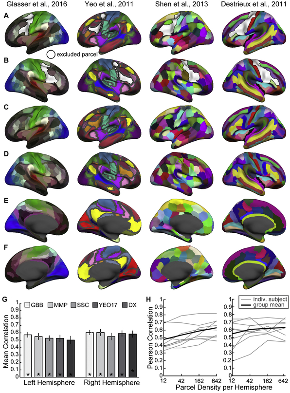
Several previously published cortical parcellations were used to define feature sets for modeling the relationship between connectivity and functional responses. The primary parcellation used to investigate various ‘connectome fingerprinting’ parameters was the Gordon et al., 2016 rsFC boundary-based parcellation (GBB; 333 parcels; downloaded from http://www.nil.wustl.edu/labs/petersen/Resources.html). Other parcellations examined included the Human Connectome Project’s (HCP) Multi-Model Parcellation (MMP; 360 total parcels; Glasser et al., 2016; downloaded from https://balsa.wustl.edu/study/show/RVVG) the Shen et al., 2013 rsFC spectral clustering parcellation (SSC; 268 total parcels; downloaded from https://www.nitrc.org/frs/?group_id=51), the 17 network parcellation of Yeo et al., 2011 (YEO17; 115 total parcels; downloaded from https://surfer.nmr.mgh.harvard.edu/fswiki/CorticalParcellation_Yeo2011) and the curvature-based parcellation of Destrieux et al., 2011 (DX; 150 total parcels; standard FreeSurfer template) (Figure 11A-F). MMP was used to investigate different regression algorithms. It has the most total parcels of any other published parcellation tested and was recently used to investigate the intrinsic connectivity of these same bilateral modality-selective LFC regions using HCP data (Tobyne et al., 2017). The YEO17 and DX parcellations are surfaced-based and available on the fsaverage surface and thus needed no modifications to adapt them for surface-based CF analyses. The GBB parcellation was resampled from fs_LR template surface (Van Essen et al., 2012) space to fsaverage cortical space using the tool ‘wb_command’ (Marcus et al., 2011) and the -label- resample function. The SSC parcellation is downloaded as a volume-based parcellation and required several preparatory steps for resampling to the cortical surface. The SSC volumetric parcellation in MNI152 space and at 2 mm resolution was first sampled to the cortical surface using wb_command’s – volume-to-surface-mapping function and the –enclosing algorithm. The resulting surface parcellation was first dilated and then eroded with wb_command’s –label-dilate and –label-erode functions, respectively, until holes within parcels or gaps between parcels were filled.

Fig. 11.

Visualization of the four group-level parcel-lations tested, in addition to Gordon et al., 2016 (see Fig. 2). (A,B) Left and right hemisphere lateral surfaces indicating the extent of excluded parcels (white), (C,D) unmasked lateral surfaces and (E,F) medial surfaces display the parcels from the various parcellation schemes. Depending upon the hemisphere analyzed, the predictor set include parcels visible on the masked ipsilateral (A or B) and the contralateral unmasked surface (C or D) as well as always included both medial surfaces (E and F). Dark gray shading indicates either unlabeled cortex from the original publication (i.e. the parcellation is made available without these vertices labelled) or non-cortex vertices (i.e. the ‘medial wall’). (G) Parcellation scheme has little effect on model accuracy. No group-based parcellation schemes performed significantly better than the others. GBB and MMP demonstrated slight perfor-mance advantages over SCC, YEO17 and DX parcel-lations, however there were no significant differences between any parcellation type in either hemisphere (left: p¼0.92; right: p¼0.98; one-way ANOVA). (H) Model performance with random parcellations of varying numbers of parcels. Paired t-tests indicated that there is a significant increase in accuracy in the left hemisphere as parcel density increases from 12 to 42 and from 42 to 162.

The correspondence between an individual’s underlying functional anatomy and a parcellation derived from group-level data may be paramount to the level of accuracy the CF modelling procedure can achieve. It is unclear to what degree the various available group-level parcellations correspond to any one individual’s unique functional topography and, furthermore, correspondence is likely to vary across the brain due to the known inter-subject variability in connectivity architecture (e.g., Mueller et al., 2013). In our paradigm, we placed less importance on inference and model coefficient interpretability in favor of optimizing the predictive power of CF modelling. To this end, we hypothesized that the level of correspondence between a subject’s functional topography and a given parcellation may not be of great importance, provided that the possible feature space (i.e. the brain) is sampled densely enough. To test this possibility, we used icosahedrons of four increasing densities (12, 42, 162 and 641 parcels per hemisphere) available from the standard FreeSurfer distribution to parcellate the cortex and serve as a set of ‘random’ features that have no explicit anatomical or functional correspondence with underlying cortical topography (Supplemental Figure 8).

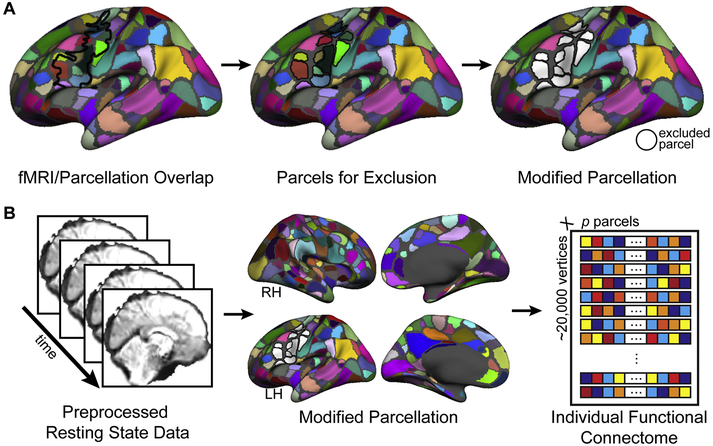
Each hemisphere’s parcellation was separately modified to exclude parcels that overlapped considerably with the search space (Figure 2A,B, Figure 11, Supplemental Figure 8). This was done to ensure that the connectivity pattern of each vertex in the search space was not biased by its inclusion in the mean time course of any target parcel. To designate a set of parcels for exclusion, we first calculated the spatial overlap between each hemisphere’s search space and all parcels of each parcellation. Any parcel that overlapped more than 50% of its area with the search space was removed from the parcellation. For parcellations based upon the FreeSurfer icosahedrons, we additionally masked the medial wall from each hemisphere’s parcellation prior to feature extraction. The number of parcels remaining for each parcellation before and after parcel exclusion, as well as the total number of parcels used as features to predict each hemisphere’s search space, is presented in Supplemental Table 1. All full and modified parcellations tested are presented in Figure 2B, Figure 11, and Supplemental Figure 8.

Fig. 2.

Parcellation modification and individual functional connectome definition. (A) A parcellation was modified by removing parcels that overlapped more than 50% with the search space. The parcellation of Gordon et al. (2016) was used in the primary ana-lyses. (B) For each hemisphere of each individual subject, a functional connectivity matrix (“individual functional connectome”) was defined from resting-state functional data by computing the Pearson correlation between the time course of each vertex of the search space and the average time course of the vertices within each parcel of the modified parcellation.

2.7. Individual Functional Connectome Definition

In order to operationally define an individual’s functional connectome for the search space, vertex-to-parcel functional connectivity was computed for every search space vertex and all non-excluded parcels of a given cortical parcellation. Each parcel’s rs-fMRI time course was first computed by averaging across all vertices within the parcel and was then correlated to that of every vertex within the search space. This was done separately for each hemisphere using the masked set of ipsilateral parcels and the full contralateral set (Figure 2B). This process results in a matrix for each subject’s hemisphere, with dimensions v by p, where v is the number of vertices in the search space and p is the number of parcels across the rest of the brain.

2.8. Multiple Regression Algorithms and Training Procedures

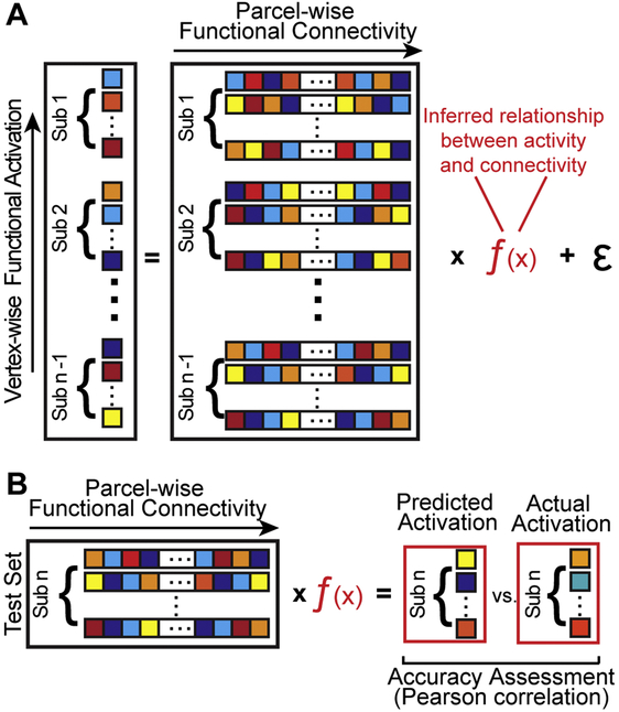
All CF regression models were implemented in MATLAB. Similar to other work (Saygin, Osher et al., 2011; Osher et al., 2016; Tavor et al., 2016; Smittenaar et al., 2016; Wang et al., 2016), a subject’s functional response to the VASA task activation (y) was conceptualized as a standard multiple linear regression problem, or the linear combination of their unique functional connectivity profile (X), which can be measured, and a set of coefficients (β), which must be inferred, plus residual error (Figure 3A), where i = 1, …, n vertices and j = 1, …, p parcels

$$y_i={\beta }_0+{\beta }_1{X}_{i1}+{\beta }_2{X}_{i2}+\cdots +{\beta }_j{X}_{ij}+{\epsilon }_i$$

We employed ridge regression (Hoerl & Kennard, 1970) or Tikhonov regularization as our primary algorithm, which places a penalty on the L2 norm of the regression coefficients. Additionally, ordinary least squares (OLS), ridge or Tikhonov regularization (Hoerl & Kennard, 1970), least absolute shrinkage and selection operator (LASSO; Tibshirani, 1996) and elastic net (Zou & Hastie, 2005) were compared using the VASA9 dataset and GBB-derived functional connectomes (see Supplemental Methods). All models were trained using a nested leave-one-subject-out cross validation procedure (Hastie, Tibshirani & Freidman, 2009) that separated model training and hyperparameter selection from model accuracy assessment (Figure 3A; Supplemental Figure 3). The resulting model is a p × 1 vector where p is the number of parcels. Briefly, for each iteration of the cross-validation procedure, one subject was selected to be left out of the model outer loop. For the OLS model training, the remaining n-1 subjects were used to train the model and there was no inner, nested loop. The OLS model was trained once using n-1 subjects and applied to the left-out subject to test model performance. The process was iterated n times; once for each subject in the dataset. For LASSO, ridge and elastic net regression algorithms, which each possess one or more hyperparameters requiring tuning, one additional subject was selected to be left out and the remaining n-2 subjects were entered into an inner loop. Models were trained on the n-2 subsample across a range of hyperparameters and the resulting models were applied to the inner loop left out subject. This process was iterated n-1 times; leaving each inner loop subject out once. Prior to assessing model performance using the outer loop left out subject, the inner loop models were aggregated and the best performing model across all inner loop models was determine by finding the minimum mean squared error across subjects. The model coefficients corresponding to this model and its associated hyperparameter(s) were then averaged across all nested loop iterations and applied to the outer loop left out subject for final performance assessment. This entire process was carried out n times; leaving each outer loop subject out once.

Fig. 3.

Overview of the connectome fingerprinting model procedure. (A) Functional responses are conceptualized as a linear regression problem from which the inferred relationship between function and connectivity can be esti-mated. A separate CF model was constructed for each subject using only the data from other subjects. Penalized regression methods used a nested leave-one-out cross-validation approach to select parameters. (B) Activation predictions were generated by applying the subject’s unique functional connectome data to the model. Prediction accuracy was assessed by a vertex-wise comparison (correlation) with actual task activation for the subject.

2.8.1. Model Predictions & Accuracy Assessment.

CF model predictions (a vector of length v) of a subject’s pattern of activation across the search space was generated by multiplying the individual’s functional connectome (i.e., vertex-to-parcel connectivity matrix) by the model, f(x), which was constructed leaving out data from that subject (Figure 3B). Each subject of the VASA9 or VAWM14 datasets, depending upon the analysis, was left out once. Accuracy metrics were calculated for each iteration of the leave-one-out cross-validation outer loop and averaged to yield an overall accuracy. Pearson correlation was used to assess the accuracy of the various model specifications was the Pearson correlation between actual and predicted task activation within the search space, for each subject hemisphere. Pearson correlations were normalized with Fisher’s r-to-Z transformation for statistical analysis. Z values were averaged and converted back to correlation values for group-level reporting purposes.

We examined whether our predictive modelling procedures were superior to a group average for predicting an individual’s activation pattern. We tested this by performing a set of leave-one-subject-out group GLM (LOSO-GLM) analyses using the VASA9 and VAWM14 datasets. All subject’s second-level t-fMRI auditory-vs-visual contrast results were first resampled to fsaverage surface space. For each iteration of the LOSO-GLM we selected one subject to be left out and performed a GLM analysis with the remaining subjects using the same procedures as in section 2.3. We performing variance smoothing (3 mm FWHM) as low-N studies are known to benefit from this procedure (Nichols & Holmes, 2002). The resulting t statistic maps for the contrast of auditory attention over visual attention were correlated to the left-out subject’s activation predicted from the CF model for each hemisphere’s search space. Correlation coefficients were Fisher r-to-Z transformed prior to statistical analysis and converted back to correlation for reporting. LOSO-GLM surface overlays were generously thresholded at p < 0.01, uncorrected, before visualization.

We examined whether an individual’s unique pattern of t-fMRI activation is best predicted by their own connectome fingerprint, compared to any other subject’s connectivity distribution. We tested this in the VASA9 and VAWM14 data by calculating the correlation between each subject’s t-fMRI activation pattern (normalized t statistics) and the predicted activation pattern obtained by applying each other subject’s functional connectome to the model. Thus, for each subject, N correlation values were calculated per hemisphere: one using the subject’s own functional connectome and N-1 others using the functional connectome of each of the remaining subjects in the respective dataset. This procedure represents a rigorous test of whether an individual’s own CF conveys a significant advantage over another subject’s CF.

The current standard for accurate reproduction of subject-specific ROIs is to use a separately acquired t-fMRI localizer that is known to recruit the same or similar regions to those of interest to the researcher (e.g. Schwarzlose, Baker and Kanwisher, 2005; Fedorenko et al., 2010; Nieto-Castanon & Fedorekno, 2012). This technique provides an independent method to localize an ROI for further analysis, but has a major drawback in that the localizer task nearly always requires multiple time consuming and expensive t-fMRI acquisitions in addition to the acquisitions for the original task. We compared the performance of the CF prediction method to the task localizer method by using the VAWM task as a separate t-fMRI localizer in seven subjects that overlapped between the VASA9 and VAWM14 datasets. For each of the 7 overlapping subjects we conducted standard GLM analysis of the VAWM task, but with a varying number of input acquisitions (1 run through 8 runs). We performed a bootstrapping procedure that sampled 100 times with replacement from each of the eight possible runs for a given iteration (e.g. 100 separate GLM analyses performed using one run sampled from the possible eight runs; 100 GLM’s sampling two runs sampled from the possible eight runs; etc.). For each subject, the Pearson correlation between their VAWM auditory-vs-visual covert attention contrast (using a variable number of t-fMRI runs) and their VASA auditory-vs-visual covert attention contrast was calculated within each hemisphere’s search space. We then estimated the average number of t-fMRI acquisitions at which the accuracy of the localizer approached the average accuracy from the connectome fingerprinting technique. In this way, the approximate number of t-fMRI acquisitions required to produce results equivalent to the connectome fingerprinting prediction from a single rs-fMRI acquisition could be assessed.

2.9. Statistical Analysis

All statistical analyses were computed with MATLAB (R2016b, The MathWorks, Natick, MA; RRID: SCR_001622). Model performance was tested for significant difference from zero with Student’s t-tests and against the LOSO-GLM analyses with paired t-tests. Significant improvement in model accuracy due to increasing the length of the resting-state time series was tested with paired t-tests. Significant differences between predicted activation and localizer accuracy, model accuracy due to regression algorithm choice or parcellation choice were performed with paired t-tests.

3. Results

3.1. Prediction Accuracy on the VASA9 Dataset

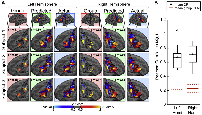
For the VASA9 dataset, we first computed each subject’s functional connectome for the LFC search space in each hemisphere, as the vertex-to-parcel correlations in resting-state fMRI data for each vertex in the LFC search space and each cortical parcel outside the LFC search space (see Methods; Figure 2). This analysis used the GBB cortical parcellation (Gordon et al. 2016). In order to predict each subject’s LFC VASA response pattern at the level of an individual vertex, we first left-out that subject’s data and constructed a CF model from the functional connectome and task activation data of all other subjects (see Methods, Figure 3A). This analysis used Tikhonov regularization (ridge regression) and a nested cross-validation procedure to optimize the regularization coefficient (see Methods, Supplemental Figure 3). The resulting CF model was then applied to the connectome data taken from within the LFC search space of the left-out subject, producing predicted VASA responses for each LFC vertex. We tested the accuracy of the CF predictions by comparing model predictions against that subject’s actual VASA task activation data. CF model accuracy was assessed by a Pearson correlation between actual and CF predicted data (separately for each hemisphere). CF model accuracy was compared against the leave-one-subject-out group-average GLM (LOSO-GLM) prediction, as assessed by Pearson correlation with the actual data. Figure 4A displays the actual, CF prediction and LOSO-GLM results for three representative subjects from the VASA9 dataset. Pearson correlation values are indicated in the CF prediction and LOSO-GLM columns. Predictions made with the GBB parcellation and using the ridge regression algorithm were highly accurate; the predicted activation patterns correlated very strongly with the actual VASA activation patterns, while the LOSO-GLM predictions did not. Results are summarized across the group in Figure 4B. The average Fisher-transformed correlation accuracy was 0.67 in the left hemisphere and 0.71 in the right hemisphere – significantly above the mean LOSO-GLM correlation of 0.18 and 0.22, respectively, and well outside their respective 95% confidence intervals (left: p<0.0001, t(8)=7.47; right: p<0.0001, t(8)=9.42; paired t-tests). Actual individual subject task activation, CF predicted activation, and LOSO-GLM group-average activation results for all VASA9 subjects are depicted in Supplemental Figure 3. For illustrative purposes, the average coefficient strength across subjects for this primary analysis are depicted in Supplemental Figure 4. For our primary analysis, we also calculated the ‘proportion of ground truth’ and Dice Coefficient of overlap as secondary accuracy metrics (see Supplemental Methods). At the threshold used in Figure 4 and Figure 7, all regions were significantly well predicted by the CF procedure (Supplemental Figure 5). Using a simple thresholding procedure to convert the model’s continuous-valued predictions into categorical ROI estimates, Dice coefficients of 0.54, 0.41, 0.37, and 0.50 were obtained for sPCS, tgPCS, iPCS, and cIFS in the left hemisphere and 0.66, 0.45, 0.47, and 0.38 in the right hemisphere, respectively (see Supplemental Figure 6).

Fig. 4.

Connectome Fingerprinting accurately predicts individual subject task activation patterns within modality-selective lateral frontal cortex in the VASA attention task. (A) Actual VASA task activation (blue background), CF predicted activation (green background), and activation predicted by a leave-one-subject-out group GLM (red background) in LFC for three example subjects. The correlation of Actual to CF Predicted and Actual to Group GLM are displayed within the respective panels. Maps were individually normalized within the LFC search space. (B) Model performance, quantified as the Pearson correlation between predicted activation and actual activation, for all subjects from the VASA9 dataset are displayed. Mean correlations (black circle) for the left and right hemispheres was 0.67 and 0.71, respectively (Fisher r-to-Z transformed). CF predictions were significantly better than the application of a LOSO group GLM (red solid lines; dashed red lines = 95% confidence interval) to the left-out subject (left: p < 0.0001, t = 7.47; right: p < 0.0001, t = 9.42; paired t-tests).

Fig. 7.

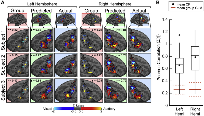
Connectome Fingerprinting accurately predicts recruitment of modality-selective lateral frontal cortex by working memory (VAWM task). (A) Actual (blue background), CF Predicted (green background) and Group GLM (red background) LFC results for three example subjects from the VAWM14 dataset. The correlation of Actual-to-Predicted and Actual-to-Group are displayed within the respective panels. Maps were individually normalized within the LFC search space. (B) Actual-to-Predicted Mean correlations (filled black circle) for the left and right hemispheres was 0.65 and 0.79 respectively (Fisher r-to-Z transformed). CF predictions were significantly better than the application of a leave-one-subject-out group GLM (solid red lines, dashed red lines = 95% confidence interval) to the left-out subject (left: p < 0.0001, t₍₁₃₎ = 4.42; right: p < 0.0001, t₍₁₃₎ = 8.64; paired t-tests).

Our primary analysis in Figure 4 excluded all parcels for which the majority of the parcel fell within our search space (see Methods). We also repeated our analysis for the GBB parcellation, excluding all parcels that had any overlap with the search space. Not surprisingly, exclusion of these regions of small overlap had negligible impact on the findings. A non-significant increase in performance was observed in the left hemisphere (0.6692 vs. 0.6723; p=0.1805; t(8)=−1.47; paired t-test) while a non-significant decrease was observed in right hemisphere (0.7125 vs. 0.7098; p=0.656; t(8)=0.4626; paired t-test).

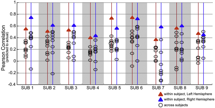
We next examined how well a subject’s own functional connectome relates to their specific VASA response pattern. We compared each subject’s VASA t-fMRI recruitment with predictions built from each other subject’s connectivity patterns (individual functional connectome) in order to assess the predictive specificity of a subject’s unique connectivity pattern. This analysis confirmed that task activation for individual VASA9 subjects were almost always (in 143 out of 144 comparisons) better predicted by their own functional connectome than by any other subject’s functional connectome, with only a single exception from one hemisphere (Figure 5). Thus, the large degree of variability across subjects’ VASA responses is well captured by the unique functional connectome of a single subject.

Fig. 5.

An individual’s LFC functional activation in the VASA task is best predicted by their own func-tional connectome. Each subject’s left (blue triangle) and right (red triangle) hemisphere prediction accu-racy (correlation between actual and predicted acti-vation) is compared to the prediction accuracy obtained using the functional connectome of each other subject (gray circles). Each subject’s own func-tional connectome data outperformed the predictions obtained using other subjects’ functional con-nectomes, with one exception (S9, RH).

3.2. CF Prediction vs. Task Localizer Performance

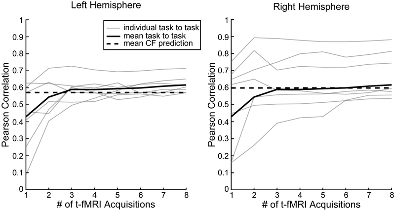
Currently, the most effective and established method for identifying regions of interest (ROIs) in individual subjects is to acquire a separate, within-subject functional localizer task dataset (e.g. Schwarzlose, Baker and Kanwisher, 2005; Fedorenko et al., 2010; Nieto-Castanon & Fedorekno, 2012). We compared the efficacy of the CF technique with the within-subject functional localizer approach. Seven subjects participated in both the VASA9 and VAWM14 datasets. Previously, Noyce et al., 2017 reported that there was a high degree of correspondence in the location of each of the four sensory-selective LFC regions between the VASA and VAWM tasks. Here, we quantified the predictive power of the within-subject task localizer by computing the Pearson correlation between the VASA and VAWM task activation across the LFC search space for these subjects. Our analysis parametrically varied the amount of VAWM task data included in the predictions, from 1 to 8 task runs. Figure 6 displays the comparison between the CF technique and the VAWM localizer task in reproducing the observed pattern of activation from the VASA task. Pearson correlation between VASA and VAWM significantly increased as additional t-fMRI runs were added (left: p<0.0001, F_(2,5)=19.22; right: p=0.05, F_(2,5)=2.25; one-way ANOVA), consistent with an increase in functional signal-to-noise with added task acquisitions. The average curve appears to asymptote at three runs in both hemispheres. The crossing point for the solid and dashed black lines indicates the number of t-fMRI acquisitions at which the VAWM localizer task, on average, equates the performance of the CF technique performed with a single rs-fMRI acquisition. In both hemispheres, the lines crossed first at three acquisitions and, notably, did not diverge much further when t-fMRI acquisition runs four through eight were added. This indicates that a single six-minute rs-fMRI acquisition run produces results on par with three 4.5-minute t-fMRI acquisition runs. In addition, there is minimal gain in acquiring five additional t-fMRI acquisition runs relative to results obtained with the single resting-state acquisition run. To identify an upper-bound on performance, we examined task replicability for the VAWM dataset by conducting separate GLM’s for odd and even runs and correlating their resulting normalized T-statistic maps (i.e. 4 odd runs vs. 4 even runs). Correlation were 0.90 in each hemisphere. This indicates that future advanced in CF methods could potentially achieve greater accuracy.

Fig. 6.

Task localizer accuracy as a function of the number of t-fMRI acquisition runs. The mean accuracy of the VAWM task localizer (thick solid line) increases with number of VAWM t-fMRI acquisition runs used, stabilizing at ~3 acquisitions. Individual subject results are shown in thin solid lines. In both hemispheres, the VAWM localizer requires 3 runs (4.5 minutes each) to equate or surpass the accuracy of the CF predictions (dashed line), which require only a single 6-minute run of rs-fMRI.

3.3. Validation of CF Technique with Visual/Auditory Working Memory Task

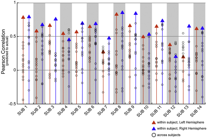
We also examined the ability of the CF technique to predict modality-selective task activation in LFC in a different task, the VAWM working memory paradigm. We examined the VAWM14 dataset using the same CF methods described above for the VASA9 dataset, including using only a single run of rs-fMRI data, but trained the model using VAWM14 data only. Our results verify that CF modelling techniques accurately predict unique patterns of modality selective functional recruitment in LFC at the individual level (Figure 7A). The mean correlation between the CF predictions and actual VAWM responses was 0.57 (p<0.0001, t(13)=9.35) in the left hemisphere and 0.66 (p<0.0001, t(13)=10.28) in the right hemisphere (Figure 7B). Similar to the VASA9 analyses, we found that the CF technique also predicts modality-selective working memory functional recruitment in LFC significantly more accurately than a group analysis (left: p < 0.0001, t(13)=5.09; right: p<0.0001, t(13)=10.52; paired t-tests). To evaluate whether individual subjects within the VAWM14 dataset are best predicted using their own functional connectome, we conducted the same analysis presented in Figure 5 on VAWM14 data. We found that VAWM14 task activation was generally better predicted by a subject’s own functional connectome than by that of any other subject (Figure 8), confirming that this premise holds for both datasets presented here. All actual surfaces, predicted surfaces, and LOSO-GLM surfaces for the VAWM14 dataset are presented in Supplemental Figure 8, for both hemispheres.

Fig. 8.

An individual’s lateral frontal cortex functional activation in the VAWM task is generally best predicted by their own functional connectome. Each subject’s left (blue triangle) and right (red triangle) correlation between actual and predicted is compared to the correlation between their actual and each other subject’s prediction (gray circles).

3.4. Effect of resting state time series length

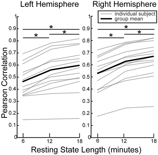
The VAWM14 dataset was used to examine CF model performance changes as the number of resting state acquisitions increased (Figure 9). The majority of VASA9 subjects possessed only 1 run of rs-fMRI data while thirteen of the VAWM14 subjects participated in three runs of a higher resolution and lower TR rs-fMRI acquisition. CF predictions were made using rs-fMRI input equal to 6-, 12-, or 18-minutes of data and compared using paired t-tests. Performance of the CF modelling method significantly increased as time series length was increased from 6-minutes to 12-minutes (left: p<0.0001, t(12)=6.49; right: p<0.0001, t(12)=10.98) and again from 12-minutes to 18-minutes (left: p<0.0001, t(12)=6.66; right: p<0.0001, t(12)=7.64). Model predictions made with 18-minutes of rs-fMRI data were significantly more accurate than those made with 6-minutes (left: p<0.0001, t(12)=6.93; right: p<0.0001, t(12)=10.16).

Fig. 9.

Effect of resting state acquisition length on CF model performance for the VAWM task. Both hemisphere’s demonstrated improvement as additional resting state acquisitions were added to the modelling procedure (all p < 0.0001; paired t-tests with Holm-Bonferroni correction). *p < 0.0001

3.5. Effect of regression algorithm, regularization and parcellation method

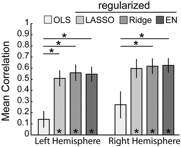
We also evaluated how the specific form of regression algorithm influenced performance of the CF technique. We hypothesized that model performance would benefit from penalized regression algorithms due to the high degree of multicollinearity present in the parcellation-based connectivity distributions. The selected models used were ordinary least squares (OLS), least absolute shrinkage and selection operator (LASSO), ridge regression (ridge), and elastic net (EN). The performance of models trained on the chosen set of linear regression algorithms using MMP-derived CFs is summarized in Figure 10. LASSO, ridge and EN each dramatically outperformed OLS (p>0.001). The performance of models trained with LASSO, ridge or EN regression algorithms were nearly indistinguishable; indicating that the connectivity distributions possess a degree of multicollinearity and the predictions benefit from some amount of regularization.

Fig. 10.

CF model performance for each form of regression algorithm. Only the three penalized regression (‘regularized’) algorithms were significantly different from zero (paired t-test). In both hemispheres, ordinary least squares (OLS) was significantly outperformed by Ridge and EN (left: p<0.0001, F = 10.45; right: p < 0.01, F = 6.09; one-way ANOVA with Tukey’s post-hoc test). LASSO significantly outperformed OLS in the left hemisphere only. LASSO = least ab-solute shrinkage and selection operator. EN = elastic net. *p < 0.01.

We evaluated how the chosen parcellation scheme affected the accuracy of the CF technique with the VASA9 dataset. The full and modified cortical parcellations used for these analyses are displayed in Figure 2B and Figure 11A-F (see Methods for additional explanation). The aggregate performance of models trained using ridge regression and the chosen set of parcellations is reported in Figure 11G. The best performing models used functional connectomes derived from the MMP and GBB parcellations, although the performance difference between parcellations was not significant (Supplemental Table 2). GBB demonstrated a slight numerical advantage for the left hemisphere, while MMP was more accurate in the right.

In addition to evaluating model performance with previously published cortical parcellations, we also tested several ‘random’ surface parcellations with varying numbers of parcels per hemisphere: 12, 42, 162, and 642. The random parcellations are available as surfaces in the standard FreeSurfer release. Performance for the left hemisphere increased with the number of parcels, while performance in the right hemisphere leveled off (Figure 11H). It is unclear whether LH performance would continue to improve at even higher parcel densities. Performance with the Random162 parcellation matched the performance of MPP, GBB, or Shen (non-significant t-tests, all p > 0.1) which have similar numbers of parcels per hemisphere (180, 167 and 134). Performance with the Random42 parcellation matched the performance of the DX and Yeo17 parcellations (non-significant paired t-tests, all p > 0.15), which have 75 and 58 parcels in a hemisphere. These results indicate that CF model performance is largely independent of the specific form of cortical parcellation assumed, so long as a sufficient number of parcels are defined.

4. Discussion

We used a regression-based modelling technique called ‘connectome fingerprinting’ (CF), first introduced by Saygin, Osher et al. (2011) to investigate whether task-free functional connectivity could predict a subject’s actual task activation. Our findings indicate that we can accurately predict the location and magnitude of functional recruitment of sensory modality-selective cognitive regions in lateral frontal cortex (LFC) during demanding attention and working memory tasks using only an individual’s unique functional connectome. Our models significantly outperformed a group analysis and predictions were significantly better when a subject’s own functional connectome was used – as opposed to any other subject’s connectome. Model accuracy was significantly improved using penalized regression but was robust across three different penalized regression paradigms. The specific choice of cortical parcellation had little impact on CF model performance, so long as a sufficient number of parcels were defined. CF predictions made with six minutes of resting state data were as accurate at reproducing a subject’s pattern of functional recruitment as a separate task localizer acquisition requiring more than twice as much data and the performance of a cognitively demanding fMRI task. Moreover, CF predictions improved with the inclusion of additional resting-state data. These findings indicate the capability of CF predictions to succeed in identifying sensory-selective frontal cortical regions, which consist of small functional regions with relatively high inter-subject variability in region location. Our results provide a blueprint for performing effective CF predictions. These updated methodologies may have applications in basic research and in precision medicine.

Connectome Fingerprint LFC predictions are as accurate as an independent task localizer

Several recent publications have revealed strong sensory biases in multiple higher order cognitive regions in lateral frontal cortex (Braga et al., 2013, 2017b; Michalka et al., 2015; Mayer et al., 2017; Noyce et al., 2017). Our results reveal that CF techniques can be used to predict sustained attention and working memory task activation in modality-selective LFC regions. We found that, for both a selective attention task paradigm (VASA) and a working memory task paradigm (VAWM), we could accurately predict both the location and magnitude of task recruitment using a subject’s own resting-state functional connectivity pattern. CF model prediction accuracy was on par with the accuracy obtained from a separately acquired task localizer. Noyce et al. (2017) previously found that LFC regions recruited by the VAWM task have a high degree of overlap with VASA regions – indicating that it is an excellent independent localizer for modality-selective regions in LFC. Predictions made using the CF technique to reproduce an individual’s pattern of activation were as good as would be indicated by the independent VAWM localizer. Furthermore, parametrically manipulating the number of t-fMRI acquisitions that were entered into the second-level GLM analysis revealed that a single 6-minute rs-fMRI acquisition could produce results as accurate as three 4.5-minute t-fMRI acquisitions – a substantial time and money savings.

Mapping lateral frontal cortex represents a significant research endeavor in neuroscience. The functional connectivity of this large section of cortex is highly variable across subjects (Mueller et al., 2013) and robust identification of an individual’s functional topography is a challenge. Much of previous research into LFC has utilized group analyses, which can obscure small, variably located regions due to group averaging effects, as in Figure 1B. For example, Mayer et al. (2016) found that 30 or more subjects were required to reliably localize several auditory- and visual-selective regions (different from those presented here) using a demanding multi-sensory Stroop task. The four bilateral LFC regions investigated here are not visible in group level analysis of this study population (Figure 1B) and demonstrate a high degree of inter-individual variability (Supplemental Figures 3 and 6); however, the pattern of four interleaved sensory-selective regions per hemisphere is fully observable in 90% of subjects. CF analyses have the power to identify these small LFC regions at the individual subject level and predict an individual’s unique topography. This represents a significant step forward in the field’s ability to reliably identify regions in LFC.

As an alternative to group level analyses, several recent publications have introduced the idea of collecting exceedingly large amount of data on individual subject’s: so-called ‘deep sampling’ (Laumann et al., 2015; Braga et al., 2017a; Gordon et al., 2017). This has the benefit of increasing the signal-to-noise for t-fMRI and rs-fMRI but comes at a dramatically increased monetary cost. Collecting such larger amounts of data is beyond the resources of most neuroimaging laboratories. Furthermore, ‘deep sampling’ methods place high demands on subjects, thus greatly limiting the application to clinical populations. CF prediction techniques may provide a happy medium between large group level studies and highly detailed individual studies by leveraging information from individual patterns of activation and connectivity from studies with a more typical sample size.

The realization that a modest amount of rs-fMRI data can be used, and reused, to accurately generate task activation patterns in individuals has a multitude of implications for basic neuroscience research. With properly trained models, researchers could forego the expensive and time-consuming process of acquiring separate task localizers when required to generate independent regions of interest. As the movement towards open science continues, researchers could also produce and accumulate CF models based upon their own in-lab datasets that other research could apply to their own data. This practice would benefit recent calls for greater transparency and openness between researchers (e.g. Poldrack et al., 2017; Nichols et al., 2017) and would facilitate the sharing of results across institutions – perhaps without the infrastructure and hosting requirements (since CF models are highly compressed linking functions between connectivity and t-fMRI with a very small data footprint) encountered by large data sharing initiatives of unprocessed data such as openfMRI (https://openfmri.org), highly preprocessed data such as Brainmap (http://www.brainmap.org) or mixed data such as the Human Connectome Project (https://humanconnectome.org). Future research will need to investigate whether CF techniques remain as accurate when applied across research settings, institutions and MRI scanners. To facilitate such work, we have made our final CF models available for download from sites.bu.edu/fmri/fingerprinting.

CF techniques hold great promise for application in the clinical setting. It is difficult to acquire data in many clinical populations for numerous reasons, including budgetary concerns, patient comfort, and data quality considerations (e.g. movement-induced artifacts). CF techniques could be applied to past and future clinical datasets that acquire only anatomical and rs-fMRI data. Connectome fingerprinting has been used to examine category selectivity in blind individuals (Wang et al., 2017) and to predict language areas in presurgical populations (Parker Jones et al., 2017). Once firmly established and validated, CF techniques could be brought into the clinic directly to study and monitor individual patients; however, much work remains to be done to achieve clinical standards for reliability and accuracy.

Further recommendations for future research and development

Prior CF analyses have employed structural (Saygin, Osher et al., 2011; Osher et al, 2016; Wang et al., 2017; Smittenaar et al., 2017) and functional (Tavor et al., 2016; Parker Jones et al., 2017) connectivity. Here, we used functional connectivity to reveal the fine-scale organization of multiple regions of two intertwined networks (visual-selective and auditory-selective) in frontal cortex. We evaluated how model accuracy changed given a set of regression algorithms and a set of cortical parcellations. Our results indicate that functional connectomes derived from any parcellation that adequately samples the functionally variable regions that make up the cortical surface can be used to make accurate predictions. These findings demonstrate that CF predictions significantly benefit from penalized regression algorithms (Figure 10). Ridge, LASSO and EN regression all produced large and significant gains over OLS regression. This likely arises from features that share similar connectivity profiles (i.e. nodes of the same network). We also found that increasing the amount of rs-fMRI data acquired provided a statistically significant advantage for CF prediction accuracy. Recent ‘deep sampling’ work suggests that approximately 20 minutes of rs-fMRI data is required to stabilize many functional connectivity measures (Gordon et al., 2017). Our work is largely consistent with this finding; however subsequent work should be conducted to extend the amount of rs-fMRI data included in the analysis past the 18-minutes tested here. Despite the accuracy gains with additional rs-fMRI acquisition, we also emphasize that a single 6-minute resting-state acquisition is sufficient to provide highly accurate predictions that are on par with a separate within-subject localizer.

5. Conclusion

In conclusion, we have demonstrated that the connectome fingerprint technique accurately predicted the functional recruitment of modality-selective lateral frontal cortex in selective attention and working memory tasks. Furthermore, these predictions are as accurate as a separately acquired task localizer, but at a substantial time and cost savings. This work is the first to provide a structured investigation of a relatively small space of the possible methodological choices available when performing CF predictions. Despite the promise connectome fingerprinting holds for basic, clinical and applied research the use of machine learning for predicting an individual’s brain topography remains in its infancy. More research and development is urgently needed to maximize the predictive power of connectome fingerprinting and realize its full potential as an investigative and diagnostic tool.

References

- Astafiev SV, Shulman GL, Stanley CM, Snyder AZ, Van Essen DC, Corbetta M (2003) Functional Organization of Human Intrparietal and Frontal Cortex for Attending, Looking, and Pointing. J Neurosci 23(11):4689–4699. [DOI] [PMC free article] [PubMed] [Google Scholar]
- Badre D (2008) Cognitive control, hierarchy, and the rostro-0caudal organization of the frontal lobes. Trends in Cog Sci 12(5): 193–200 [DOI] [PubMed] [Google Scholar]
- Behzadi Y, Restom K, Liau J, Liu TT (2007) A component based noise correction method (CompCor) for BOLD and perfusion based fMRI. NeuroImage 37:90–101. [DOI] [PMC free article] [PubMed] [Google Scholar]
- Braga RM, Buckner RL (2017a) Parallel Interdigitated Distributed Networks within the Individual Estimated by Intrinsic Functional Connectivity. Neuron 95(2):457–471. [DOI] [PMC free article] [PubMed] [Google Scholar]
- Braga RM, Hellyer PJ, Wise RJS, Leech R (2017b) Auditory and Visual Connectivity Gradients in Frontoparietal Cortex. Hum Brain Mapp, 38(1):255–70. [DOI] [PMC free article] [PubMed] [Google Scholar]
- Brainard DH (1997) The Psychophysics Toolbox. Spat Vis 10(4):433–436.9176952 [Google Scholar]
- Carp J (2013) Optimizing the order of operations for movement scrubbing: Comment on Power et al. NeuroImage 76:436–438. [DOI] [PubMed] [Google Scholar]
- Dale AM, Fischl B, Sereno MI (1999) Cortical Surface-Based Analysis. I: Segmentation and Surface Reconstruction. NeuroImage 9(2):179–194. [DOI] [PubMed] [Google Scholar]
- Destrieux C, Fischl B, Dale A, Halgren E (2010) Automatic parcellation of human cortical gyri and sulci using standard anatomical nomenclature. NeuroImage 53:1–15. [DOI] [PMC free article] [PubMed] [Google Scholar]
- Fedorenko E, Duncan J, Kanwisher J (2013) Broad domain generality in focal regions of frontal and parietal cortex. Proc Natl Acad Sci USA 110(41):16616–16621. [DOI] [PMC free article] [PubMed] [Google Scholar]
- Fedorenko E, Hsieh PJ, Nieto-Castañón A, Whitfield-Gabrieli S, Kanwisher N (2010) New method for fMRI investigations of language: defining ROIs functionally in individual subjects. J Neurophysiol 104(2), 1177–1194. http://doi.org/10.1152/jn.00032.2010 [DOI] [PMC free article] [PubMed] [Google Scholar]
- Feinberg DA, Setsompop K (2013) Ultra-fast MRI of the human brain with simultaneous multi-slice imaging. J Magn Reson 229:90–100. [DOI] [PMC free article] [PubMed] [Google Scholar]
- Fischl B (2012) FreeSurfer. Neuroimage 62(2): 774–781. [DOI] [PMC free article] [PubMed] [Google Scholar]
- Fischl B, Sereno MI, Dale AM (1999) Cortical Surface-Based Analysis. II: Inflation, Flatterning, and a Surface-Based Coordinate System. NeuroImage 9(2):195–207. [DOI] [PubMed] [Google Scholar]
- Friston KJ, Willians S, Howard R, Frackowiak RSJ, Turner R (1996) Movement-Related effects in fMRI time-series. Magn Reson Med 35(3):346–355. [DOI] [PubMed] [Google Scholar]
- Glasser MF, Coalson TS, Robinson EC, Hacker CD, Harwell J, Yacoub E, Ugurbil K, Andersson J, Beckmann CF, Jenkinson M, Smith SM, Van Essen DC (2016) A multi-modal parcellation of human cerebral cortex. Nature 536(7615):171–178. [DOI] [PMC free article] [PubMed] [Google Scholar]
- Gordon EM, Laumann TO, Adeyemo B, Huckins JF, Kelley WM, Petersen SE (2016) Generation and Evaluation of a Cortical Area Parcellation from Resting-State Correlations. Cereb Cortex 26(1):288–303. [DOI] [PMC free article] [PubMed] [Google Scholar]
- Gordon EM, Laumann TO, Gilmore AW, Newbold DJ, Greene DJ, Berg JJ, Ortega M, Hoyt-Drazen C, Gratton C, Sun H, Hampton JM, Coalson RS, Nguyen AL, McDermott KB, Shimony JS, Shyder AZ, Schlagger BL, Pertersen SE, Nelson SM, Dosenbach NUF (2017) Precision Functional Mapping of Individual Human Brains. Neuron 95(4):791–807. [DOI] [PMC free article] [PubMed] [Google Scholar]
- Greve DN, Fischl B (2009) Accurate and robust brain image alignment using boundary-based registration. NeuroImage 48(1):63–72. [DOI] [PMC free article] [PubMed] [Google Scholar]
- Hallquist MN, Hwang K, Luna B (2013) The nuisance of nuisance regression: Spectral misspecification in a common approach to resting-state fMRI preprocessing reintroduces noise and oscures functional connectivity. NeuroImage 82:208–225. [DOI] [PMC free article] [PubMed] [Google Scholar]
- Hastie T, Tibshirani R, Friedman J (2009) The Elements of Statistical Learning: Data Mining, Inference, and Prediction, New York, NY: Springer. [Google Scholar]
- Hoerl AE, Kennard R (1970) Ridge regression: Biased estimation for nonorthogonal problems. Technometrics 12:55–67. [Google Scholar]
- Kleiner M, Brainard D, Pelli D (2007) What’s new in Psychtoolbox-3? Perception 36 ECVP Abstract Supplement. [Google Scholar]
- Koechlin E, Ody C, Kouneiher F (2003) The Architecture of Cognitive Control in the Human Prefrontal Cortex. Science 302(5648):1181–1185. [DOI] [PubMed] [Google Scholar]
- Laumann TO, Gordon EM, Adeyemo B, Snyder AZ, Joo SJ, Chen MY, Gilmore AW, McDermott KB, Nelson SM, Dosenbach NUF, Schlaggar BL, Mumford JA, Poldrack RA, Petersen SE (2015) Functional System and Areal organization of a Highly Sampled Individual Human Brain. Neuron 87(3):657–670. [DOI] [PMC free article] [PubMed] [Google Scholar]
- Marcus DS, Harwell J, Olsen T, Hodge M, Glasser MF, Prior F, Jenkinson M, Laumann T, Curtiss SW, Van Essen DC (2011) Informatics and data mining tools and strategies for the Human Connectome Project. Front Neuroinform 5(4). DOI:10.3389.fninf.2011.00004. [DOI] [PMC free article] [PubMed] [Google Scholar]
- Mayer AR, Ryman SG, Hanlon FM, Dodd AB, Ling JM (2017). Look Hear! The Prefrontal Cortex is Strtified by Modality of Sensory Input During Multisensory Cognitive Control. Cereb Cortex 27(5):2831–2840. [DOI] [PMC free article] [PubMed] [Google Scholar]
- Michalka SW, Kong L, Rosen ML, Shinn-Cunningham BG, Somers DC (2015) Short-Term Memory for Space and Time Flexibly Recruit Complementary Sensory-Biased Frontal Lob Attention Networks. Neuron 87(4):882–892. [DOI] [PMC free article] [PubMed] [Google Scholar]
- Mueller S, Wang D, Fox MD, Yeo BTT, Sepulcre J, Sabuncu MR, Shafee R, Lu J, Liu H (2013) Individual Variability in Functional Connectivity Architecture of the Human Brain. Neuron 77:586–595. [DOI] [PMC free article] [PubMed] [Google Scholar]
- Mugler JP, Brookeman JR (1991) Rapid three-dimensional T1-weighted MR imaging with the MP-RAGE sequence. J Magn Reson Imaging 1(5):561–567. [DOI] [PubMed] [Google Scholar]
- Nee DE, D’Esposito M (2016) The hierarchical organization of the lateral prefrontal cortex. eLife 5:e12112 DOI: 10.7554/eLife.12112. [DOI] [PMC free article] [PubMed] [Google Scholar]
- Nichols TE, Das S, Eickhoff SB, Evans AC, Glatard T, Hanke M, Kriegeskorte N, Milham MP, Poldrack RA, Poline J-B, Proal E, Thirion B, Van Essen DC, White T, Yeo BTT (2017) Best practices in data analysis and sharing in neuroimaging using MRI. Nat Rev Neurosci 20:299–303 [DOI] [PMC free article] [PubMed] [Google Scholar]
- Nichols TE, Holmes AP (2002) Nonparametric Permutation Tests For Functional Neuroimaging: A Primer with Examples. Hum Brain Mapp 15(1):1–25. [DOI] [PMC free article] [PubMed] [Google Scholar]
- Nieto-Castanon A, Fedorenko E (2012) Subject-specific functional localizers increase sensitivity and functional resolution of multi-subject analyses. NeuroImage 63(3):1646–1669. [DOI] [PMC free article] [PubMed] [Google Scholar]
- Noyce AL, Cestero N, Michalka SW, Shinn-Cunningham BG, Somers DC (2017) Sensory-Biased and Multiple-Demand Processing in Human Lateral Frontal Cortex. J. Neurosci 37(36):8755–8766. [DOI] [PMC free article] [PubMed] [Google Scholar]
- Osher DE, Saxe RR, Koldewyn K, Gabrieli JDE, Kanwisher N, Saygin ZM (2016) Structural Connectivity Fingerprints Predict Cortical Selectivity for Multiple Visual Categories across Cortex. Cereb Cortex 26:1668–1683. DOI: 10.1093/cercor/bhu303. [DOI] [PMC free article] [PubMed] [Google Scholar]
- Parker Jones O, Voets NL, Adcock JE, Stacey R, Jbabdi S (2017) Resting connectivity predicts task activation in pre-surgical patients. NeuroImage: Clinical 13:378–385. [DOI] [PMC free article] [PubMed] [Google Scholar]
- Petrides M (1995) Functional organization of the human frontal cortex for mnemonic processing. Evidence from neuroimaging studies. Ann N Y Acad Sci 769:85–96. [DOI] [PubMed] [Google Scholar]
- Poldrack RA, Baker CI, Jurnez J, Gorgolewski KJ, Matthews PM, Munafo MR, Nichols TE, Poline J-B, Vul E, Yarkoni T (2017). Scanning the horizon: towards transparent and reproducible neuroimaging research. Nat Rev Neurosci 18:115–126. [DOI] [PMC free article] [PubMed] [Google Scholar]
- Power JD, Barnes KA, Snyder AZ, Schlaggar BL, Petersen SE (2012) Spurious but systematic correlations in functional connectivity MRI networks arise from subject motion. NeuroImage 59:2142–2154. [DOI] [PMC free article] [PubMed] [Google Scholar]
- Power JD, Mitra A, Laumann TO, Snyder AZ, Schlaggar BL, Petersen SE (2014) Methods to detect, characterize, and remove motion artifact in resting state fMRI. NeuroImage 84:320–341. [DOI] [PMC free article] [PubMed] [Google Scholar]
- Power JD, Schlaggar BL, Petersen SE (2015) Recent progress and outstanding issues in motion correction in resting state fMRI. NeuroImage 105:536–551. [DOI] [PMC free article] [PubMed] [Google Scholar]
- Sallet J, Mars RB, Noonan MP, Neubert FX, Jbabdi S, O’Reilly JX, Filippini N, Thomas AG, Rushworth MF (2013) The Organization of Dorsal Frontal Cortex in Humans and Macaques. J Neurosci 33(30):12255–12274. [DOI] [PMC free article] [PubMed] [Google Scholar]
- Saygin ZM, Osher DE, Koldewyn K, Reynolds G, Gabrieli DJE, Saxe RR (2011) Anatomical connectivity patterns predict face selectivity in the fusiform gyrus. Nat Neurosci 15(2):321–327. [DOI] [PMC free article] [PubMed] [Google Scholar]
- Schwarzlose RF, Baker CI, Kanwisher N (2005) Separate Face and Body Selectivity on the Fusiform Gyrus. J Neurosci 25(47):11055–11059. [DOI] [PMC free article] [PubMed] [Google Scholar]
- Setsompop K, Gagoski BA, Polimeni JR, Witzel T, Wedeen VJ, Wald LL (2012) Blipped-Controlled Aliasing in Parallel Imaging for Simultaneous Multislice Echo Planar Imaging With Reduced g-Factor Penalty. Magn Reson Med 67:1210–1224. [DOI] [PMC free article] [PubMed] [Google Scholar]
- Shen X, Tokuglu F, Papademetris X, Constable RT (2013) Groupwise wole-brain parcellation from resting-state fMRI data for network node identification. NeuroImage 82:403–415. [DOI] [PMC free article] [PubMed] [Google Scholar]
- Smittenaar P, Kurth-Nelson Z, Mohammadi S, Weiskopf N, Dolan RJ (2017) Local striatal reward signal can be predicted from corticostriatal connectivity. NeuroImage 159:9–17. [DOI] [PMC free article] [PubMed] [Google Scholar]
- Tavor I, Jones OP, Mars RB, Smith SM, Behrens TE, Jbabdi S (2016) Task-free MRI predicts individual differences in brain activity during task performance. Science 352(6282):216–220. [DOI] [PMC free article] [PubMed] [Google Scholar]
- Tibshirani R (1996) Regression shrinkage and selection via the lasso. J Royal Statist Soc B 58(1):267–288. [Google Scholar]
- Tobyne SM, Osher DE, Michalka SW, Somers DC (2017) Sensory-biased attention networks in human lateral frontal cortex revealed by intrinsic functional connectivity. NeuroImage 162:362–372. [DOI] [PMC free article] [PubMed] [Google Scholar]
- Van Essen DC, Glasser MF, Dierker DL, Harwell J, Coalson T (2012) Parcellations and hemispheric asymmetries of human cerebral cortex analyzed on surface-based atlases. Cereb Cortex 22(10):2241–2262. [DOI] [PMC free article] [PubMed] [Google Scholar]
- Wang X, He C, Peelen MV, Zhong S, Gong G, Caramazza A, Bi Y (2017) Domain Selectivity in the Parahippocampal Gyrus Is Predicted by the Same Structural Connectivity Patterns in Blind and Sighted Individuals. J Neurosci 37(18):4705–4716. [DOI] [PMC free article] [PubMed] [Google Scholar]
- Yeo BTT, Krienen FM, Sepulcre J, Sabuncu MR, Laskari D, Hollinshead M, Roffman JL, Smoller JW, Zollei L, Polimeni JR, Fischl B, Liu H, Buckner RL (2011) The organization of the human cerebral cortex estimated by intrinsic functional connectivity. J Neurophysiol 106(3):1125–1165. [DOI] [PMC free article] [PubMed] [Google Scholar]
- Zou H, Hastie T (2005) Regularization and variable selection via the elastic net. J Royal Statist Soc B 67:301–320. [Google Scholar]
Associated Data
This section collects any data citations, data availability statements, or supplementary materials included in this article.