Compartmental Model Diagrams as Causal Representations in Relation to DAGs

Abstract

Compartmental model diagrams have been used for nearly a century to depict causal relationships in infectious disease epidemiology. Causal directed acyclic graphs (DAGs) have been used more broadly in epidemiology since the 1990s to guide analyses of a variety of public health problems. Using an example from chronic disease epidemiology, the effect of type 2 diabetes on dementia incidence, we illustrate how compartmental model diagrams can represent the same concepts as causal DAGs, including causation, mediation, confounding, and collider bias. We show how to use compartmental model diagrams to explicitly depict interaction and feedback cycles. While DAGs imply a set of conditional independencies, they do not define conditional distributions parametrically. Compartmental model diagrams parametrically (or semiparametrically) describe state changes based on known biological processes or mechanisms. Compartmental model diagrams are part of a long-term tradition of causal thinking in epidemiology and can parametrically express the same concepts as DAGs, as well as explicitly depict feedback cycles and interactions. As causal inference efforts in epidemiology increasingly draw on simulations and quantitative sensitivity analyses, compartmental model diagrams may be of use to a wider audience. Recognizing simple links between these two common approaches to representing causal processes may facilitate communication between researchers from different traditions.

Introduction

Epidemiology aims to understand disease causation in addition to disease associations (Bradford Hill (1965)). Causal directed acyclic graphs (DAGs), developed and popularized by Pearl, Robins, Greenland and others (Greenland, Pearl, and Robins (1999), Hernán, Hernández-Díaz, Werler, and Mitchell (2002), Glymour (2008), Hogan (2009)), have been used broadly in epidemiology since the late 1990s (Joffe, Gambhir, Chadeau-Hyam, and Vineis (2012)). This use of Bayes nets to represent causal processes allows for the determination of conditional independencies of random variables under a proposed causal structure. Compartmental model diagrams, also known as flow diagrams (Forrester (1970)), have long been used to depict causal processes in infectious disease epidemiology (e.g. Kermack and McKendrick (1932)). These diagrams explicitly represent the dynamics of the variables on a DAG, and implicitly specify their joint distributions. Both types of diagrams can depict causal processes (Joffe et al. (2012), Commenges and Gégout-Petit (2009)). The correspondence between the two types of diagrams has been underexplored, however, and many practitioners do not recognize the link between these two approaches. While causal DAGs are useful in reasoning through study design and analytic issues, compartmental model diagrams provide a visual but precise representation of a dynamical system. A compartmental model diagram is a formal object that represents an underlying dynamical system and can also represent a causal structure in the counterfactual framework. We show how to use compartmental model diagrams to parametrically express the same concepts as DAGs. While DAGs more concisely depict causation, mediation, confounding, and collider bias, compartmental model diagrams explicitly depict dynamical relationships and interactions. A compartmental model diagram can aid in translating the causal structure in a DAG into equations that can be analyzed or programmed, or into code for stochastic or deterministic simulation in discrete or continuous time.

Methods and Results

Definitions

Counterfactuals

In the counterfactual framework of causation, each individual has a set of counterfactual outcomes corresponding to potential outcomes under each possible exposure, where outcomes may be conceived of as either deterministic or stochastic. Only the counterfactual outcome corresponding to the exposure received is realized. Suppose random variable Y represents the realized outcome under exposure received. We can also define the random variable Y^a, the counterfactual outcome under treatment a; a is a member of some set of treatments and A is a random variable taking on values in this set. y^a denotes a single realization of Y^a. (For example, y¹ might denote an individual’s counterfactual dementia status in the present if they had diabetes at an evaluation 10 years ago, and y⁰ would denote that individual’s counterfactual dementia status in the present if they had not had diabetes at an evaluation 10 years ago. If the individual did not have diabetes at an evaluation 10 years ago, then y⁰ corresponds to their realized outcome.) In this framework, a causal effect for the ith individual is defined to be $y_i^{a=1}-y_i^{a=0}$, if outcomes are deterministic, and $E[Y_i^{a=1}]-E[Y_i^{a=0}]$, if outcomes are stochastic (Greenland et al. (1999), VanderWeele and Robins (2012)). Individual-level causal risk differences can be averaged over a population to obtain population-level causal risk differences. Equivalently, causal effects can be defined in terms of a risk or odds ratio.

DAGs

We briefly review DAGs; a comprehensive review of DAGs and their use in epidemiology can be found elsewhere (Greenland et al. (1999), Glymour (2008)). In a causal DAG, nodes represent random variables, while arrows represent causal effects. Acyclic graphs are used to depict causal relations, because it is assumed that cause precedes effect. By convention, when we consider an analysis or sample selection that conditions on a variable, we indicate this in a DAG by putting a box around that variable. Similar graphs are frequently used informally to represent conceptual models or statistical patterns, but, with a set of formal rules, the diagrams can be much more informative. Specifically, a causal DAG has the following features (Hernán and Robins (2016, forthcoming)):

1. The lack of arrow between two nodes indicates a lack of a direct causal effect,

2. All common causes of any pair of variables are on the graph, and

3. A variable is a cause of all of its descendants, where descendant is defined as follows: a variable Y is a descendant of a variable X if and only if there is a directed path from X to Y, where a directed path is a path in which all arrows point in the same direction, and, in this case, towards Y and away from X.

We focus on causal DAGs; non-causal DAGs will not be treated further in this paper.

Figure 1 depicts a DAG in which the random variable A causes the random variable Y. This DAG represents the assumption that no common causes of A and Y exist, because none are shown. A DAG implies a set of conditional independencies, determined by the d-separation criteria, which are defined elsewhere and are used to determine which variables on a DAG are statistically independent conditional on other variables (Hernán and Robins (2016, forthcoming), Glymour (2008)). A DAG is said to faithfully represent a set of conditional independencies if and only if that DAG implies those and only those conditional independencies (Hernán and Robins (2016, forthcoming), Spirtes, Glymour, and Scheines (2000)).

Figure 1.

Causal DAG representing that random variable A causes random variable Y, with no common causes of A and Y.

Single world intervention graphs are elaborations of DAGs that depict counterfactuals and thus can be used to infer counterfactual independence relations (Richardson and Robins (2013)). A single world intervention graph can be used to show the DAG in figure 1 also implies Y^a is independent of A, or Y^a ⫫A. For dichotomous A, the two groups corresponding to A = 0 and A = 1 are said to be exchangeable if and only if Y^a⫫A. If, when conditioning on a set of confounders C, A and Y are d-separated, then Y^a ⫫A|C. For dichotomous A, the two groups corresponding to A = 0 and A = 1 are said to be conditionally exchangeable on C if and only if Y^a⫫A|C (Hernán and Robins (2016, forthcoming), Glymour (2008)).

Compartmental Model Diagrams

While the use of Bayes nets to represent causal models has become an important part of statistical analysis of epidemiologic data, there is a long tradition of compartmental model diagrams (also known as flow diagrams) that can represent the values of the joint distributions of the variables in a DAG. Compartmental model diagrams are widely used to depict the flow of individuals or objects through different possible states (e.g. Forrester (1970)), and can be used to represent many types of mathematical structures. We will focus on one of the most common uses: to represent state variables (variables corresponding to the number of individuals in a given state, such as susceptible, infected, and removed/recovered as a function of time) in a stochastic process. State variables are by convention represented as capital letters (e.g. S, I, R) and are functions of time. At times, the time dependence is implied: that is, S(t) is simply written S (e.g. Allen, Brauer, Van den Driessche, and Wu (2008), Edelstein-Keshet (1988)).

The compartments, or nodes, in a compartmental model diagram correspond to numbers of individuals in each of the possible states an individual in the population can inhabit, and the arrows indicate the possible transitions between states. An individual can move from any compartment to any other provided an arrow points from one to the other. The arrow labels on a compartmental model diagram define the waiting time distribution for the corresponding transition. We abbreviate whenever possible: If the diagram represents a continuous-time Markov model (jump process), in which an individual’s instantaneous rates of transition to other states from a given state are independent of how long the individual was in that state and all previous states, arrows will be labeled with per capita flow rates. If the waiting times are deterministic, we can label arrows with those waiting times. In the remainder of the paper, compartmental models diagrams will depict Markov models unless otherwise noted.

Note that while compartmental model diagrams are represented by labeled directed graphs, the graphs are not acyclic in general. Compartmental model diagrams in the literature do not follow a standardized form: some authors represent states as rectangles (e.g. Kermack and McKendrick (1932)), others circles (e.g. Enanoria, Worden, Liu, Gao, Ackley, Scott, Deiner, Mwebaze, Ip, Lietman, and Porco (2015)); some label arrows with total flow rates (e.g. Ackley, Liu, Porco, and Pepperell (2015)), others with per-capita flow rates (e.g. Andersen and Keiding (2002)), and others do not label arrows at all (e.g. Lipsitch, Cohen, Cooper, Robins, Ma, James, Gopalakrishna, Chew, Tan, Samore et al. (2003)). In a compartmental model diagram, some rates may be the sum of positive and negative quantities, in which case they can be conceptualized as flows going in both directions. In addition, rates may be zero, in which case the arrow is omitted. Multiple arrows going from one state to another can always be combined into a single arrow whose label is the sum of the labels on the original multiple arrows, and we assume that any compartmental model diagram has been reduced to this form.

Given a state X in a model with some flow rate λ out of that state into another state, the corresponding stochastic model is formed by assuming that each individual in state X experiences a hazard (i.e. instantaneous flow rate) λ of undergoing the transition to the other state. Two or more arrows out of state X, for example an arrow to Y and and arrow to Z, are assumed to represent processes, which are conditionally independent given state X (Norris (1998)).

Counterfactual waiting times correspond to the amount of time an individual would remain in a given state X conditional on transitioning to each of the possible transitions out of X (Norris (1998), Gillespie (1977)). We call these waiting times counterfactual waiting times since not all corresponding events occur. For an individual in a given state, multiple transitions are often possible from that state. For any stochastic realization of the model for which an individual is in state X, the transition that occurs is the transition with the shortest counterfactual waiting time for that realization. Suppose we have a compartmental model diagram, in which individuals in state X can transition to states Y and Z at average per-individual rates of λ and μ. In such a compartmental model diagram, the probability that an individual who transitions experiences a transition to Y is the standard competing risk formula λ/(λ + μ). For a stochastic realization, each individual i has counterfactual waiting times corresponding to the waiting times to states Y and Z. If the counterfactual waiting time to state Y is shorter than the counterfactual waiting time to state Z, then the individual transitions to Y, and if the counterfactual waiting time to state Y is longer than the counterfactual waiting time to state Z, the individual transitions to Y.

A simple example compartmental model diagram is shown in figure 2. Consider individuals who have been exposed (A = 1) or unexposed (A = 0) to some putative risk factor at baseline. We wish to model the occurrence of a binary outcome variable, Y = 0 or Y = 1, over time. We define four state variables for this system: N_A=a,Y=y for each possible combination of a and y, where a corresponds to a specific value of A (0 or 1) and y corresponds to a specific value of Y (0 or 1). Individuals with A = 0 proceed from a state with Y = 0 (N_A=0,Y=0) to a state with Y = 1 (N_A=0,Y=1) at an average rate of α, whereas individuals with A = 1 proceed from a state with Y = 0 (N_A=1,Y=0) to a state with Y = 1 (N_A=1,Y=1) at an average rate of β. These rates imply that, within a small time step Δt, the number of individuals who transition from a state with A = 0, Y = 0 to a state with A = 0, Y = 1 may be approximated by a binomially-distributed random variable with denominator N_A=0,Y=0 and probability αΔt, and the number of individuals who transition from a state with A = 1, Y = 0 to a state with A = 1, Y = 1 may be approximated by a binomially-distributed random variable with denominator N_A=1,Y=0 and probability βΔt. Compartmental model diagrams with time-constant rates will also imply exponentially distributed waiting times for individuals to transition from one compartment to another.

Figure 2.

Compartmental model diagram showing that individuals with A = 0 proceed from Y = 0 to Y = 1 at a rate of α, whereas individuals with A = 1 proceed from Y = 0 to Y = 1 at a rate of β.

Compartmental model diagrams are depictions of a mechanistic process (Commenges and Gégout-Petit (2009), Aalen, Røysland, Gran, and Ledergerber (2012)). While the precise relationship between mechanism and causation is debated, some have argued that a mechanistic understanding implies a causal understanding (Commenges and Gégout-Petit (2009), Aalen et al. (2012)): “The interventionist and mechanistic viewpoints are by no means entirely separate…. In a sense, mechanisms represent the structure of the world, and the aim of human intervention is to gain understanding of this structure to exploit it for some purpose. The mechanisms in the structure of the world are present whether humans are there to intervene or not, and hence seem to be the more fundamental aspect” (Aalen et al. (2012)). In a compartmental model diagram that fully depicts this underlying mechanism, moving an individual from one compartment to another implies a new trajectory with a potentially different hazard of leaving that compartment. Thus, the compartmental model diagram implies the counterfactual definition of causation and thus is a causal diagram. In addition, all causes are on the graph, since the underlying mechanism is fully depicted, and therefore, all common causes are on the graph. In the practice of epidemiologic modeling, compartmental models may omit some real-world causes of transition either because not all causes are known or because some factors are not thought to significantly affect dynamics. Such a model represents a simplified version of reality that is nonetheless a causal model, even if incomplete or incorrect.

In constructing a compartmental model diagram, certain aspects of the process are included based on an understanding of the underlying causal process. If the rate describing the transition from one state to another is not a function of another variable in the system, then we are indicating that that variable is not causal for that transition. For example, if, in figure 2, α =β, we are indicating that transitions to Y = 1 states are independent of the exposure A, but are nonetheless an important part of the dynamical process. However, if α ≠ β, we are indicating that values of A are causally related to transitioning to Y = 1 states.

Diagrams Related to DAGs

We focus on DAGs in contrast to compartmental model diagrams, but there are several types of causal diagrams related to DAGs that merit exploration: Local independence graphs depict marked point processes. Since these graphs are not required to be acyclic, they can depict feedback between variables (Didelez (2008, 2007)). Single-world intervention graphs display factual and counterfactual random variables on the same graph. These graphs are useful in determining the counterfactual independence relations implied by a DAG (Richardson and Robins (2013)). Chain graphs are graphs with both directed and undirected edges, but do not allow partially directed cycles. Undirected edges are used to model simultaneous responses, feedback relationships, non-causal associations, or uncertainty about the direction of the causal relationship (Lauritzen and Richardson (2002)). Acyclic directed mixed graphs are used to model random variables that have been marginalized over undepicted latent variables. These graphs have both directed and bidirected edges, and do not allow cycles of directed edges. These graphs are closed under marginalization, whereas DAGs are not (Evans, Richardson et al. (2014)). Structural equation models are frequently used to model unobserved constructs and can be represented with DAGs where the edges are labeled with partial correlation coefficients; such diagrams can useful in parameterizing DAGs (Knott and Bartholomew (1999)).

Each of these diagrams is useful, particularly in contexts where DAGs may be insufficient. However, all are closely related to DAGs and fundamentally different than compartmental model diagrams. In compartmental model diagrams, the nodes represent the number of individuals in a given state and not variables corresponding to characteristics of individuals.

Corresponding Compartmental Model Diagrams and DAGs

In many circumstances, the same underlying process can be represented by a compartmental model diagram and by a DAG since compartmental model diagrams can represent the values of the joint distributions of the variables in a DAG. If a compartmental model diagram and DAG both imply the same conditional independencies (for both factual and counterfactual variables), we will refer to them as corresponding.

We note that more than one compartmental model diagram can correspond with a given DAG for two reasons: First, there are infinite ways to parameterize a single compartmental model diagram. Second, structurally different compartmental model diagrams may correspond to the same DAG, though some correspondent compartmental model diagrams can be ruled out on substantive grounds. For example, the compartmental model diagram in figure 2 and a slightly different compartmental model diagram that allowed for the acquisition of the exposure at a rate γ with the inclusion of arrows from N_A=0,Y=0 to N_A=1,Y=0 and N_A=0,Y=1 to N_A=1,Y=1, would both correspond to the DAG in figure 1 equally well. Whether the acquisition of the exposure after baseline is implausible and the latter compartmental model diagram can be ruled out will depend on the exposure A. In addition, a compartmental model diagram can indicate the distinct causal effects of an exposure on both the onset and resolution of disease, which is not easily represented in a DAG. This use of compartmental model diagrams can be found in the disability literature (e.g. Bardenheier, Lin, Zhuo, Ali, Thompson, Cheng, and Gregg (2016).)

We also note that a compartmental model diagram may correspond with more than one DAG, depending how one chooses to define random variables of interest. For example, a compartmental model diagram that depicts the rates at which individuals with and without dementia die could correspond equally well to a DAG that depicts dementia causing death by some fixed time point and a DAG that depicts dementia affecting the waiting time until death.

Nonetheless, corresponding DAGs and compartmental model diagrams may have certain features. A corresponding compartmental model diagram can be constructed from a DAG as follows: for a DAG with n dichotomous variables, a corresponding compartmental model diagram could be constructed by depicting 2ⁿ compartments that correspond to all of the possible states in which an individual could exist. This is trivially extended for polychotomous variables where a DAG with n polychotomous variables, where the ith variable has m_i possible values. A corresponding compartmental model diagram would have ${\prod }_{i=1}^n{m}_i$ states. A compartmental model diagram of a Markov process may depict additional intermediate states in order to alter the distribution of waiting times for a transition (Granich, Gilks, Dye, De Cock, andWilliams (2009)).

Using counterfactual waiting times, it is possible to prove that the conditional independencies implied by a compartmental model diagram are the same conditional independencies implied by a DAG if the two diagrams are corresponding. These proofs are included in the appendix.

Example Corresponding DAGs and Compartmental Model Diagrams

Using an example from chronic disease epidemiology, we now illustrate corresponding compartmental model diagrams and DAGs representing alternate structures linking type 2 diabetes to dementia. We assume variables of different letters are not equal. While we note that hazard ratios can have built-in selection bias (frailty bias) (Hernán, Hernández-Díaz, and Robins (2004)) in other settings, the hazard ratios read off a compartmental model diagram do correctly characterize the causal effect since all individuals in a compartment are exchangeable.

No Causation

We might imagine that there is no causal link between type 2 diabetes (abbreviated T2D in diagrams) and dementia (abbreviated D in diagrams). Figures 3(a) and (b), respectively, show a DAG and compartmental model diagram corresponding to this hypothesis. In the DAG, type 2 diabetes status is independent of dementia status. In the compartmental model diagram, individuals develop dementia at a rate α and type 2 diabetes at a rate γ. The fact that the rates of developing dementia and diabetes are the same for individuals with and without diabetes and dementia, respectively, indicates no causal effects. We now illustrate that this compartmental model diagram implies statistical independence for the random variables in the above DAG.

Figure 3.

Corresponding (a) DAG and (b) compartmental model diagram for no causation.

Suppose we are following a cohort of N people with and without diabetes, but without dementia, at baseline. Suppose a fraction f do not have diabetes at baseline. Suppose the random variables on the DAG in 3(a) corresponds to diabetes and dementia status at some specific time t^*. Solving the differential equations implied by the compartmental model diagram above gives the following for the four state variables at time t:

$$\begin{gathered} N_{T2D=0,D=0}(t)=\mathit{fN}exp(-(\alpha +\gamma )t) \\ {N}_{T2D=1,D=0}(t)=-\mathit{fN}exp(-(\alpha +\gamma )t)+Nexp(-\gamma t) \\ {N}_{T2D=0,D=1}(t)=-\mathit{fN}exp(-(\alpha +\gamma )t)+\mathit{fN}exp(-\alpha t) \\ {N}_{T2D=1,D=1}(t)=\mathit{fN}exp(-(\alpha +\gamma )t)-Nexp(-\gamma t)-\mathit{fN}exp(-\alpha t)+N \end{gathered}$$

The causal odds ratio at t =t^* is given by $\frac{N_{T2D=0,D=0}(t^{\ast })N_{T2D=1,D=1}(t^{\ast })}{N_{T2D=1,D=0}(t^{\ast })N_{T2D=0,D=1}(t^{\ast })}=1$, for all t^* > 0.

Causation

Individuals with type 2 diabetes are more likely to develop dementia. One possible explanation for this is that type 2 diabetes causes dementia (Crane, Walker, Hubbard, Li, Nathan, Zheng, Haneuse, Craft, Montine, Kahn et al. (2013)). Figures 4(a) and (b), respectively, show a DAG and compartmental model diagram corresponding to this hypothesis. In the DAG, type 2 diabetes has a causal effect on dementia. In the compartmental model diagram, individuals without type 2 diabetes progress to dementia at a rate α, whereas individuals with type 2 diabetes progress to dementia at a rate β. The fact that these rates are specified using different parameters allows for a causal effect of type 2 diabetes on dementia: individuals with type 2 diabetes develop dementia with a hazard β/α times those without type 2 diabetes. However, the rates of developing type 2 diabetes are the same (γ) for individuals with and without dementia. Note that the DAG in figure 4 has the same form as a local independence graph (see Didelez (2008)).

Figure 4.

Corresponding (a) DAG and (b) compartmental model diagram for causation.

Mediation

One explanation for why type 2 diabetes might cause dementia is that type 2 diabetes causes cerebrovascular disease (abbreviated CD in diagrams), which, in turn, causes dementia (Ahtiluoto, Polvikoski, Peltonen, Solomon, Tuomilehto, Winblad, Sulkava, and Kivipelto (2010)). In the DAG shown in figure 5(a), the causal effect of type 2 diabetes on dementia is fully mediated by cerebrovascular disease. In the corresponding compartmental model diagram in figure 5(b) we show both causal processes: the development of cerebrovascular disease and the development of dementia. We show that individuals with type 2 diabetes develop cerebrovascular disease at a rate δ whereas individuals without type 2 diabetes develop cerebrovascular disease at a rate γ. This indicates a causal effect of type 2 diabetes on cerebrovascular disease. Individuals with cerebrovascular disease, irrespective of type 2 diabetes status, develop dementia at a rate of β, whereas individuals without cerebrovascular disease, irrespective of type 2 diabetes status, develop dementia at a rate α. This indicates a causal effect of cerebrovascular disease on dementia. We note that the controlled direct effect here is null, since individuals with and without diabetes progress to dementia states at the same rate conditional on cerebrovascular disease. We also note that since there are no transitions to states with type 2 diabetes, there are no causes of type 2 diabetes represented in this compartmental model diagram.

Figure 5.

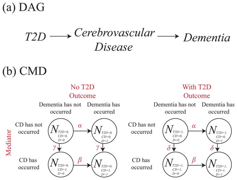
Corresponding (a) DAG and (b) compartmental model diagram for mediation. Cerebrovascular disease is abbreviated CD.

Confounding

An alternate explanation for the observed association between type 2 diabetes and the development of dementia is that some confounding factor is a common cause of both. For example, early life socioeconomic status (abbreviated SES in diagrams), might increase risk of development type 2 diabetes and may also independently increase the risk of developing dementia (Glymour (2013)). In the DAG in figure 6(a), we show that early life socioeconomic status is a common cause of type 2 diabetes and dementia. In the compartmental model diagram in figure 6(b), we show that within strata of early life socioeconomic status, there is no causal effect of type 2 diabetes on dementia since the rates of transition to dementia states are described with one parameter. However, early life socioeconomic status causes type 2 diabetes since individuals with low socioeconomic status develop type 2 diabetes at a rate γ, whereas individuals with high socioeconomic status develop type 2 diabetes at a rate δ. Furthermore, this compartmental model diagram indicates that early-life socioeconomic status causes dementia, since individuals with low socioeconomic status develop dementia at a rate α, whereas individuals with high socioeconomic status develop dementia at a rate β.

Figure 6.

Corresponding (a) DAG and (b) compartmental model diagram for confounding. Socioeconomic status is abbreviated SES.

Collider Bias

It is also possible that differential survival among those with and without type 2 diabetes and dementia affects the observed association between type 2 diabetes and dementia (Mayeda, Haan, Yaffe, Kanaya, and Neuhaus (2015a), Mayeda, Haan, Kanaya, Yaffe, and Neuhaus (2013)). In the DAG in figure 7, we show that type 2 diabetes influences survival and that dementia influences survival. Analyses, however, are restricted to individuals surviving to the time of our study (a specific way to condition on survival), as indicated by the box around survival. In the compartmental model diagram in figure 7, we show that type 2 diabetes does not cause dementia and dementia does not cause type 2 diabetes. This is because rates corresponding to horizontal arrows (the rates of developing dementia) are equal, and rates corresponding to vertical arrows (the rates of developing type 2 diabetes) are equal. However, rates of mortality, μ₀₀, μ₁₀, μ₀₁, and μ₁₁, differ for each combination of type 2 diabetes and dementia status. If we then calculated an odds ratio using surviving individuals are sampled at a time t = t^*, given by $\frac{N_{T2D=0,D=0,S=1}(t^{\ast })N_{T2D=1,D=1,S=1}(t^{\ast })}{N_{T2D=0,D=1,S=1}(t^{\ast })N_{T2D=1,D=0,S=1}(t^{\ast })}$, we would obtain an odds ratio not equal to one, despite the fact that the compartmental model diagram indicates that type 2 diabetes is not causal for dementia and dementia is not causal for type 2 diabetes.

Figure 7.

Corresponding (a) DAG and (b) compartmental model diagram for collider bias. S = 1 indicates surviving, whereas S = 0 indicates dead.

Interaction

In the next example, we again consider the situation where type 2 diabetes causes dementia. We also consider that therapy given for type 2 diabetes also has a causal effect on dementia and that therapy additionally modifies the causal effect of type 2 diabetes on dementia (Mayeda, Whitmer, and Yaffe (2015b), Mayeda, Haan, Neuhaus, Yaffe, Knopman, Sharrett, Griswold, and Mosley (2014)). By drawing arrows to therapy states for individuals without type 2 diabetes, we are allowing for the possibility that some individuals without type 2 diabetes are on therapy, perhaps due to misdiagnosis. There is no agreed upon convention to depict interaction in DAGs. Thus, the DAG shown in figure 8(a) is consistent with both compartmental model diagrams shown in figures 8(b) and 8(c).

Figure 8.

(a) DAG which corresponds equally well to (b) a compartmental model diagram showing no interaction on the multiplicative scale or (c) a compartmental model diagram showing interaction on the multiplicative scale. Therapy is abbreviated T.

In the compartmental model diagram in figure 8(b), we indicate the causal effect of type 2 diabetes on dementia by indicating that within strata of therapy the rates of acquiring dementia are γ times larger for individuals with type 2 diabetes. Furthermore, we indicate that therapy has a causal effect on dementia by noting that, within strata of type 2 diabetes status, individuals on therapy develop dementia at a rate of β times those not on therapy. Reading off the compartmental model diagram, we can see that there is no interaction on the multiplicative scale between type 2 diabetes and therapy in the development of dementia since the hazard ratios for the effect of therapy on dementia are the same among those with and without type 2 diabetes and the hazard ratios for the effect of type 2 diabetes on dementia are the same among those on or off therapy (γ). However, there is necessarily interaction on the additive scale.

In the compartmental model diagram in figure 8(c), we indicate the causal effect of type 2 diabetes on dementia by indicating that in the no therapy group the rate of acquiring dementia is γ times larger for individuals with type 2 diabetes and in the therapy group the rate of acquiring dementia is βγ times larger for individuals with type 2 diabetes. Thus, there is interaction on the multiplicative scale between type 2 diabetes and therapy in the development of dementia since therapy modifies the rate of acquiring dementia among those with type 2 diabetes, but does not modify the rate of acquiring dementia among those without type 2 diabetes. For the same reasons, we expect interaction on the additive scale.

Causation and Reverse Causation

Finally, suppose we want to express the concept that type 2 diabetes causes dementia, but also that dementia causes type 2 diabetes, perhaps due to decreased self-care among those with cognitive impairment (Fontbonne, Berr, Ducimetière, and Alpérovitch (2001)). Since a graph indicating this by drawing an arrow from type 2 diabetes to dementia and an arrow back from dementia to type 2 diabetes would not be acyclic, we must indicate this relationship with a longitudinal DAG. In figure 9(a), we show that dementia status at time 1 affects type 2 diabetes at time 2 and that type 2 diabetes status at time 1 affects dementia status at time 2, and so on. The corresponding compartmental model diagram shown in figure 9(b), both horizontal and vertical pairs of arrows are unequal, indicating that type 2 diabetes causes dementia and dementia causes type 2 diabetes, respectively.

Figure 9.

Corresponding (a) DAG and (b) compartmental model diagram for causation and reverse causation.

Infinitesimal Limit of a Longitudinal DAG

We now show that in certain cases the limit of a longitudinal population-level DAG, as the time between successive nodes goes to zero, is a compartmental model diagram. We use a simple example of the susceptible-infectious-susceptible (SIS) model of trachoma developed by Lietman et al. (Lietman, Gebre, Ayele, Ray, Maher, See, Emerson, Porco, TANA Study Group et al. (2011)). In figure 10(a) we show the DAG for this system, where I_τ gives the population-level prevalence of infection at time τ. Compartmental model diagrams are parametric (or semi-parametric) and thus require additional assumptions to be fully specified. Thus, with specific assumptions, we now show that this DAG in figure 10(a) implies the compartmental model diagram for an SIS model in figure 10(c).

Figure 10.

Corresponding (a) DAG, (b) fully specified DAG, and (c) compartmental model diagram for an SIS model of trachoma.

Suppose I_τ affects I_τ+1 via two pathways as shown in figure 10(b): first, since individuals remain infected over time, some individuals will remain infected from one time step to the next. Second, there will be a change in the number infected which is a function of only the current number infected. Thus, I_τ an be written as I_τ−1 and a change term:

$$I_{\tau }=I_{\tau -1}+{\mathrm{\Delta }}_{\tau }$$ (1)

where Δ_τ is defined to be the change in the number infected from time τ−1 to time τ. (While the DAG in figure 10(b) represents this, it depicts deterministic relations, which can lead to faithfulness violations (Spirtes et al. (2000))). The DAG in 10(b) implies Δ_τ is a function of I_τ−1, but does not specify what that function is. Now suppose individuals are conserved; that is, there are no births or deaths and no migration. Therefore, the we can write S_τ, the number of susceptible individuals at time τ, as N − I_τ where N is the time invarying size of the population. We now have:

$$\begin{gathered} I_{\tau }=I_{\tau -1}+{\mathrm{\Delta }}_{\tau } \\ {S}_{\tau }=S_{\tau -1}-{\mathrm{\Delta }}_{\tau } \end{gathered}$$

By convention, rates are non-negative. Thus, the function Δ_τ might be decomposed into new infections X_τ and recoveries Y_τ, also functions of I_τ−1, such what Δ_τ = X_τ −Y_τ. Then if we assume that X_τ and Y_τ are Poisson-distributed random variables, this implies a compartmental model diagram with the arrow from S to I labeled with X(t) and an arrow from I to S with Y(t), where X(t) and Y(t) are mean rates as a function of time. X_τ and Y_τ correspond to new infections and recoveries, respectively.

Then, if we assume X_τ and Y_τ have means βS_τ I_τΔt and γI_τΔt, respectively, where Δt is the time increment between successive measurements, as the time increment goes to zero, this implies a compartmental model diagram with average per individual rates of transition βI and γ from S to I and from I to S, respectively. Then, in the large number limit, we obtain the following set of ordinary differential equations:

$$\begin{gathered} \frac{dI}{dt}=\beta SI-\gamma I \\ \frac{dS}{dt}=-\beta SI+\gamma I \end{gathered}$$

Causal Modeling and Faithfulness

Compartmental model diagrams are especially useful for depicting causal processes in which violations of faithfulness are plausible, i.e. situations in which there are multiple, perfectly or nearly perfectly offsetting mechanisms. Using the example from Koski and Noble (2011), suppose the conditional independencies for four random variables x₁, x₂, x₃, and x₄ are as follows (and that no other conditional independencies hold):

1. x₁ ⫫ x₄|{x₂, x₃}

2. x₁ ⫫ x₄

3. x₂ ⫫ x₃|x₁

Koski and Noble (2011) show that this system of independencies can not be represented in DAG form. An example compartmental model diagram that implies these and only these conditional independencies, along with a proof, is given in the appendix.

Non-Markovian Process Models

Compartmental model diagrams may, of course, represent processes more general than Markov processes on a finite state space. Many such generalizations are available, ranging from partial differential equations (e.g. M’Kendrick (1926)) through agent-based models (Macal and North (2010), Galea, Riddle, and Kaplan (2010)). Previous examples were of models of Markov processes. We now extend our discussion to semi-Markov processes, in which the evolution of successive states follows a Markov chain, but the waiting times are not necessarily exponential (Karlin and Taylor (1975)).

In the example given in figure 11(b), arrow labels represent deterministic waiting times. We saw earlier in the No Causation example that when waiting times are exponential, the process was Markovian and the exposure and outcome were independent at all times. In the analogous semi-Markov process depicted above, the transition times are still unconditionally independent of the past sequence of states and the waiting times in those states. However, the exposure A and outcome Y are no longer independent at all times, necessitating the DAG given in 11(a).

Figure 11.

Corresponding (a) DAG and (b) CMD depicting deterministic waiting times (semi-Markovian). Suppose we perform a simulation with transitions occurring after exactly α and β time units to Y = 1 states and A = 1 states from entry into a compartment or the start of simulation. Suppose α > β. Individuals starting out with A = 0 and Y = 0 take α +β to reach a Y = 1 state, whereas individuals starting out with A = 1 and Y = 0 will take β to reach a Y = 1 state.

Generalized SIR Model

In the SIR model, each individual would be subjected to a (time-varying) jump process from S to I and I to R. The SIR model represents the evolving number of people in each of these states over time. More generally, a compartmental model diagram may be refined to a model featuring a density evolving in time. For example, to extend the SIR model to a continuous state space, we might replace the simple jump process at the individual-level with an explicit representation of the number of infectious organisms x and immune response y (e.g. Rvachev (1972)). In such an approach, each individual would follow a trajectory on the phase plane as illustrated in figure 12. The population-level SIR model is then replaced by equations representing the evolving population density of individuals in the xy-plane (equations not shown) (Metz and Diekmann (2014)).

Figure 12.

Generalized SIR model showing the trajectory of an infectious individual through the xy-plane, where x is the number of pathogens and y is the immune response. For example, an infected individual might follow a trajectory through the the plane according to the following coupled differential equations: $\stackrel{.}{x}=\frac{1}{2}\frac{x}{r}-\frac{1}{10}\frac{xy}{r}$ and $\stackrel{.}{y}=\frac{1}{2}\frac{x}{r}-\frac{1}{10}\frac{y}{r}$, where $r=\sqrt{x^2+y^2}$. The origin (blue dot) corresponds to susceptible, the y-axis with y > 0 corresponds to recovered, and all other points such that x > 0 and y ≥ 0 correspond to infectious (example trajectory in green).

We can display such a process graphically with a vector field, as shown in figure 12. In this diagram, the x-axis gives the number of infectious organisms in a host and the y-axis gives the host’s level of immune response. Susceptible corresponds to the origin (blue), removed corresponds to the y-axis with y > 0 (red), and infectious corresponds to any point on the xy plane such that x > 0 and y ≥ 0. A susceptible individual would be moved to a point on the positive x-axis by a transmission event, then be moved within the xy-plane by the immune response and pathogen dynamics, and finally end up on the y-axis (recovered). An example trajectory corresponding to a single infectious person is shown in green. The discrete DAG would necessarily be replaced by a continuous object of some kind, because individuals would not be assigned cleanly into S, I, and R, but rather to a continuous space of states. Similar considerations could be applied to other epidemic models, such as the SIS model.

Discussion

Compartmental model diagrams have found widespread use in transmission modeling due to the dynamical relationships inherent in infectious disease (Dietz (1992), Bailey (1979), Gao, Lietman, and Porco (2015)). They have also been used in chronic disease epidemiology (e.g. Murray (2002), Hardy, Dubin, Holford, and Gill (2005)). These models can be used to compare competing causal structures (e.g. Smith and Gröhn (2015)). We show that, for a set of problems, DAGs and compartmental model diagrams can both express causation, mediation, confounding, and collider bias, while compartmental model diagrams can explicitly depict interaction and depict feedback cycles.

Process models, as depicted with compartmental model diagrams, confer specific advantages for representing certain types of causal structures. First, compartmental model diagrams can depict causal processes in the presence of interference, i.e. one individual’s treatment or exposure affecting another’s outcome (Halloran, Longini, Struchiner, and Longini (2010)). Causal inference techniques and DAGs usually require the assumption of non-interference (Glymour (2008), Hernán and Robins (2016, forthcoming)), although attempts have been made to extend causal inference techniques and the DAG framework to situations with interference (Halloran and Struchiner (1995), Ogburn, VanderWeele et al. (2014), Hudgens and Halloran (2012)). Figure 10(c) depicts the SIS model, a simple epidemic model of infection followed by recovery. Epidemic models such as this depict the presence of interference with a rate that is a function of another state variable; here, the per-capita rate of infection is βI, a function of the number infected I. Therefore, interventions to reduce the number infected, such as treatment, will affect the the risk of infection for susceptible individuals. In contrast, in the diabetes-dementia examples, there is no interference because all rates are constant and thus are independent of all state variables. Second, compartmental model diagrams can explicitly depict interaction, as shown in figure 8. (DAGs are a non-parametric method and thus were not designed to represent such features.) In addition, compartmental model diagrams can depict causation and reverse causation (time-varying confounding), as shown in figure 9.

Simulation is useful for quantifying biases in statistical methods under realistic conditions in epidemiology (Bellan, Dushoff, Galvani, and Meyers (2015)) and evaluating whether hypothetical causal structures are consistent with observed data under realistic conditions (Mayeda et al. (2016)). A compartmental model diagram can aid in translating the causal structure in a DAG into equations that can be analyzed or programmed, or into code for stochastic or deterministic simulation. As outlined in the proofs in the appendix, it is often possible to represent a causal process as a DAG and corresponding CMD that can be proven to imply the same set of conditional independencies. We note that DAGs can also be parameterized, as in structural equation modeling, to help guide simulations. However, conventional approaches to parameterizing DAGs do not depict interaction, interference, or the underlying dynamical process.

Compartmental model diagrams also have some important limitations. They are not necessarily parsimonious, especially as the state space becomes large, and reading off the conditional independencies is not necessarily trivial (see proofs in Corresponding Compartmental Model Diagrams and DAGs in the appendix). Just as DAGs are not designed to display interaction, CMDs are not designed to be readable in this manner. In addition, while we have shown that compartmental model diagrams can easily depict the joint distribution of discrete random variables, these diagrams are not designed to depict the joint distributions of continuous random variables. Lastly, a DAG or related non-parametric graph might be preferable in situations where one does not wish to develop or parameterize a compartmental model diagram.

In this paper, we omitted discussion of several related topics. We focused on the stochastic process interpretation of compartmental model diagrams, though these diagrams can be used to depict other mathematical structures, such as the ordinary differential equations in Ackley et al. (2015) and the deterministic difference equations in Hargrove and Williams (1998). In addition, we focused on two commonly used graphical representations in epidemiology—DAGs and compartmental model diagrams. We only briefly discussed alternative graphical approaches related to DAGs, such as local independence graphs, chain graphs, acyclic directed mixed graphs, and structural equation models. These graphs can be used to address some of the limitations of DAGs: for example, local independence graphs can be used to parsimoniously represent feedback cycles and time-varying confounding (see examples in Didelez (2008)).

Although DAGs have become commonplace as a training tool in epidemiology, and are a near-essential component of modern causal inference literature, compartmental model diagrams have predominated in research and training on modeling of the dynamics of infectious disease outbreaks. A clear understanding of the correspondence of compartmental model diagrams and DAGs will facilitate collaboration and communication between researchers in these different traditions. We illustrate that compartmental model diagrams can parametrically express the same concepts DAGs can, as well as interaction and feedback cycles. As causal inference efforts in epidemiology increasingly draw on simulations and quantitative sensitivity analyses, compartmental model diagrams may be of use to a wider audience.

Appendix

Corresponding Compartmental Model Diagrams and DAGs

Using the compartmental model diagrams and DAGs shown in figures 1 and 2, we prove that the compartmental model diagrams also imply conditional independence and conditional exchangeability, respectively. The proofs for other factual and counterfactual dependency relationships implied by the DAGs in figures 1 and 2 follow a similar form and are thus omitted.

Proposition, Conditional Independence

Figure 1.

Corresponding (a) DAG and (b) compartmental model diagram showing confounding in the absence of a direct causal effect.

The DAG in figure 1(a) implies Y ⫫ A|C: Y and A are independent conditional on C.

Proposition

The compartmental model diagram in figure 1(b) also implies Y ⫫ A|C.

Proof

We restrict our discussion of the compartmental model diagram to individuals who are in Y = 0 states at the start of observation. Individuals who are in Y = 1 states at the start of observation do not yield information on this conditional independency, since these individuals all have outcome Y = 1 independent of all other variables in the analysis.

We define the relationship between factual outcomes and counterfactual waiting times in this example is as follows: Suppose the random variable representing the counterfactual waiting time for transitioning to an Y =1 state for individual i with A = 0 and Y = 0 is given by T_i[Y = 1]. The individual transitions to a Y = 1 state if T_i[Y = 1] < t^*, where t^* is the total observation time. Therefore, the factual outcome Y_i for that individual is given by I_Ti[Y=1]<t^*, where I is an indicator function taking on the value of one if T_i[Y = 1] < t^*, and zero otherwise.

Suppose an individual is in an A = 0, C = 0, and Y = 0 state. This individual has a constant hazard of α of moving to a Y = 1 state. Suppose an individual is in an A = 1, C = 0, Y = 0 state. This individual also has a constant hazard of α of moving to a Y = 1 state. Therefore, T_i[Y = 1|A = 0,C = 0] = T_i[Y = 1|A = 1,C = 0] = T_i[Y = 1|C = 0]. Similarly, we can show T_i[Y = 1|A = 0,C = 1] = T_i[Y = 1|A = 1,C = 1] = T_i[Y = 1|C = 1]. Therefore, by the definition of independence, T_i[Y = 1] ⫫ A|C. Since transformations of independent random variables are independent (e.g. Stone (1996), chapter 1), Y_i ⫫ A|C for each individual i. Therefore, Y ⫫ A|C.

Proposition, Conditional Exchangeability

In figure 2(a), with the addition of the arrow from A to Y, we can see that Y ⫫ A|C is false. However, this DAG implies Y^a ⫫ A|C, where Y^a is the counterfactual outcome Y under exposure a.

Proposition

The compartmental model diagram shown in figure 2(b) also implies Y^a ⫫ A|C.

Proof

We use the letter f to denote the probability density function of a continuous random variable. We define the random variable $T_i^a[Y=1]$ to be the counterfactual waiting time to a Y =1 state for the ith individual setting the exposure to a specific value A = a. The distribution of counterfactual waiting times given C = c and setting A = a is given by:

$$f(T_i^a[Y=1]=t\mid C=c,Y=0)=\sum _{\alpha \in U_A}{I}_{A_i=\alpha }f(T_i[Y=1]=t\mid A=a,C=c,Y=0)$$ (2)

where U_A is the support of A and A_i is the value of A for the ith individual; in this case, U_A = {0, 1}. In this expression, if for individual i, if A_i = a, then the distribution of counterfactual waiting times is the same as the distribution of factual waiting times. If A_i ≠ a, then we assign a distribution of counterfactual waiting times as if A = a.

Figure 2.

Corresponding (a) DAG and (b) compartmental model diagram showing confounding in the presence of a direct causal effect.

Simplifying equation 2, we have

$$f(T_i^a[Y=1]=t\mid C=c,Y=0)=f(T[Y=1]=t\mid A=a,C=c,Y=0)$$ (3)

Thus, the distribution of counterfactual waiting times setting A = a do not depend on factual values of A within C = c; they only depend on the value a we set. Therefore,

$$T_i^a[Y=1]⫫A\mid C$$ (4)

Equation 4 implies that $I_{(T_i^a[Y=1]\mid A=a)<t^{\ast }}⫫A\mid C$. Substituting $Y_i^a$ for $I_{T_i^a[Y=1]<t^{\ast }}$, we have shown $Y_i^a⫫A\mid C$ for all individuals i. Therefore, Y^a ⫫ A|C.

Causal Modeling and Faithfulness

We show that there are a set of conditional independencies that cannot be faithfully represented with a DAG (Koski and Noble (2011)), but can be represented with a compartmental model diagram. The conditional independencies for the random variables x₁, x₂, x₃, and x₄ are as follows:

1. x₁ ⫫ x₄|{x₂, x₃}

2. x₁ ⫫ x₄

3. x₂ ⫫ x₃|x₁

Figure 3.

The DAG in (a) is not faithful to the given conditional independencies. However, for a specific set of random variables this compartmental diagram does imply the given conditional independencies.

The proof that these conditional independencies cannot be represented with a DAG, and specifically the DAG given in figure 3(a), is given elsewhere (Koski and Noble (2011)). The compartmental model diagram in 3(b) represents a model in which the probability of transition in each time step of length 1 is given by the arrow labels. Suppose all individuals start in N₀₀₀₀ or N₁₀₀₀ at time zero. Suppose we define x₁ to be a random variable corresponding to whether the individual is in a state with a first subscript of 1 at time zero, x₁ and x₂ the second and third subscript at time 1, respectively, and x₄ the fourth subscript at time 2. We impose the additional constraint that a ≠ b. We now show that this compartmental model model diagram implies the above conditional independencies:

1. Probability of progression to states corresponding to x₄ = 1 is the same for individuals with a given combination of x₂ and x₃ for both x₁ = 0 and x₁ = 1. Therefore, x₄ ⫫ x₁|x₂, x₃.

2. The probability of x₄ equal to 1 is given by (a−ab)c+abd +(b−ab)c and is the same for individuals starting in N₀₀₀₀ and N₁₀₀₀ states. Thus, x₁ ⫫ x₄.

3. For x₁ = 0, the probability of x₂ = 1 is a−ab+ab = a, the probability of x₃ = 1 is b−ab+ab = b. The probability of x₂ = 1 and x₃ = 1 is ab. This implies x₂ ⫫ x₃|x₁ = 0. Similarly, we can show x₂ ⫫ x₃|x₁ = 1. Therefore, x₂ ⫫ x₃|x₁.

We now show that the compartmental model diagram does not imply any other conditional independencies. Proofs by contradiction:

1. x₁ ⫫ x₂

   P(x₂ = 1|x₁ = 0) = a and P(x₂ = 1|x₁ = 1) = b. Therefore, x₁⫫̸x₂.

2. x₁ ⫫ x₃

   Proof follows a form similar to 1, replacing x₂ with x₃.

3. x₂ ⫫ x₃

   $$\begin{gathered} P(x_2=1{\cap }_3=0) \\ =P(x_2=1\cap x_3=0\mid x_1=0)P(x_1=0)+P(x_2=1\cap x_3=0\mid x_1=1)P(x_1=1) \\ =(a-ab)P(x_1=0)+(b-ab)P(x_1=1) \\ =aP(x_1=0)+bP(x_1=1)-ab \end{gathered}$$

   This cannot be simplified further. Therefore, x₂⫫̸x₃.

4. x₂ ⫫ x₄

   $$\begin{gathered} P(x_2=1\cap x_4=1) \\ =P(x_2=1\cap x_4=1\mid x_1=0)P(x_1=0)+P(x_2=1\cap x_4=1\mid x_1=1)P(x_1=1) \\ =((a-ab)c+\mathit{abd})P(x_1=0)+((b-ab)c+\mathit{abd})P(x_1=1) \\ =(a-ab)cP(x_1=0)+(b-ab)cP(x_1=1)+\mathit{abd} \end{gathered}$$

   This cannot be simplified further. Therefore, x₂⫫̸x₄.

5. x₃ ⫫ x₄

   Proof follows a form similar to 4, replacing x₂ with x₃.

6. x₁ ⫫ x₂|x₃

   $P(x_2=1\mid x_1=0\cup x_3=0)=\frac{a-ab}{1-b}=a$, and $P(x_2=1\mid x_1=1\cup x_3=0)=\frac{b-ab}{1-a}=b$. Therefore, x₁⫫̸x₂|x₃.

7. x₁ ⫫ x₃|x₂

   Proof follows a form similar to 6, replacing x₂ with x₃ and x₃ with x₂.

8. x₁ ⫫ x₂|x₄

   $P(x_2=1\mid x_1=0\cup x_3=0)=\frac{a-ab}{1-b}=a$, and $P(x_2=1\mid x_1=1\cup x_3=0)=\frac{b-ab}{1-a}=b$. Therefore, x₁⫫̸x₂|x₃.

9. x₁ ⫫ x₃|x₄

   Proof follows a form similar to 8, replacing x₂ with x₃.

10. x₂ ⫫ x₃|x₄

    $P(x_2=1\cup x_3=0\mid x_4=1)=\frac{(a-ab)c}{(a+b-2ab)c+\mathit{abd}}P(x_1=0)+\frac{(b-ab)c}{(a+b-2ab)c+\mathit{abd}}P(x_1=1)$

    $P(x_2=1\cup x_3=0\mid x_4=0)=\frac{(a-ab)(1-c)}{1-(a+b-ab)+(a+b-2ab)(1-c)+ab(1-d)}P(x_1=0)+\frac{(b-ab)(1-c)}{1-(a+b-ab)+(a+b-2ab)(1-c)+ab(1-d)}P(x_1=1)$. Therefore, x₂⫫̸x₃|x₄.

11. x₂ ⫫ x₄|x₁

    P(x₂ = 1∩x₄ = 1|x₁ = 0) = (a−ab)c+abd

    P(x₂ = 1|x₁ = 0) = a

    P(x₄ = 1|x₁ = 0) = (a−ab)c+abd+(b−ab)c

    P(x₂ = 1∩x₄ = 1|x₁ = 0) ≠ P(x₂ = 1|x₁ = 0)P(x₄ = 1|x₁ = 0). Therefore, x₂⫫̸x₄|x₁.

12. x₃ ⫫ x₄|x₁

    Proof follows a form similar to 11, replacing x₂ with x₃.

13. x₂ ⫫ x₄|x₃

    P(x₄ =1|x₂ =0∩x₃ =1)=c and P(x₄ =1|x₂ =1∩x₃ =1)=d. Therefore, x₃⫫̸x₄|x₁.

14. x₃ ⫫ x₄|x₂

    Proof follows a form similar to 13, replacing x₂ with x₃ and x₃ with x₂.

15. x₁ ⫫ x₂|{x₃, x₄}

    $P(x_2=0\mid x_1=0\cap x_3=1\cap x_4=1)=\frac{b-ab}{(a+b-2ab)c+\mathit{abd}}$

    $P(x_2=0\mid x_1=1\cap x_3=1\cap x_4=1)=\frac{b-ab}{(a+b-2ab)c+\mathit{abd}}$. Therefore, x₁ ⫫̸ x₂|x₃, x₄.

16. x₁ ⫫ x₃|{x₂, x₄}

    Proof follows a form similar to 15, replacing x₂ with x₃ and x₃ with x₂.

17. x₂ ⫫ x₃|{x₁, x₄}

    $P(x_2=1\cap x_3=0\mid x_1=0,x_4=1)=\frac{c}{2c+d}$

    $P(x_2=1\mid x_1=0,x_4=1)=\frac{c+d}{2c+d}$

    $P(x_3=0\mid x_1=0,x_4=1)=\frac{c}{2c+d}$

    ∴ P(x₂ = 1∩x₃ = 0|x₁ = 0, x₄ = 1) ≠ P(x₂ = 1|x₁ = 0, x₄ = 1)P(x₃ = 0|x₁ = 0, x₄ = 1))

    ∴ x₂⫫̸x₃|{x₁, x₄}

18. x₂ ⫫ x₄|{x₁, x₃}

    $P(x_2=1\cap x_4=1\mid x_1=0,x_3=1)=\frac{\mathit{abd}}{b}=ad$

    $P(x_2=1\mid x_1=0,x_3=1)=\frac{ab}{b}=a$

    P(x₄ = 1|x₁ = 0, x₃ = 1) = abd + (b − ab)c

    ∴ x₂⫫̸x₄|{x₁, x₃}

19. x₃ ⫫ x₄|{x₁, x₂}

    Proof follows a form similar to 18, replacing x₂ with x₃ and x₃ with x₂.

20. x₄ ⫫ x₁|x₂

    P(x₄ =1|x₂ =1)=P(x₁ =0)((a−ab)c+abd)+P(x₁ =1)((b−ab)c+abd)

    P(x₄ = 1|x₂ = 1, x₁ = 0) = ((a−ab)c+abd)

    ∴ x₄⫫̸x₁|x₂

21. x₄ ⫫ x₁|x₂

    Proof follows a form similar to 20, replacing x₂ with x₃.

References

- Aalen OO, Røysland K, Gran JM, Ledergerber B. Causality, mediation and time: a dynamic viewpoint. Journal of the Royal Statistical Society: Series A (Statistics in Society) 2012;175:831–861. doi: 10.1111/j.1467-985X.2011.01030.x. [DOI] [PMC free article] [PubMed] [Google Scholar]
- Ackley SF, Liu F, Porco TC, Pepperell CS. Modeling historical tuberculosis epidemics among Canadian First Nations: effects of malnutrition and genetic variation. PeerJ. 2015;3:e1237. doi: 10.7717/peerj.1237. [DOI] [PMC free article] [PubMed] [Google Scholar]
- Ahtiluoto S, Polvikoski T, Peltonen M, Solomon A, Tuomilehto J, Winblad B, Sulkava R, Kivipelto M. Diabetes, Alzheimer disease, and vascular dementia a population-based neuropathologic study. Neurology. 2010;75:1195–1202. doi: 10.1212/WNL.0b013e3181f4d7f8. [DOI] [PubMed] [Google Scholar]
- Allen LJ, Brauer F, Van den Driessche P, Wu J. Mathematical epidemiology. Springer; 2008. [Google Scholar]
- Andersen PK, Keiding N. Multi-state models for event history analysis. Statistical Methods in Medical Research. 2002;11:91–115. doi: 10.1191/0962280202SM276ra. [DOI] [PubMed] [Google Scholar]
- Bailey NTJ. Introduction to the modelling of venereal disease. Journal of Mathematical Biology. 1979;8:301–322. doi: 10.1007/BF00276315. [DOI] [PubMed] [Google Scholar]
- Bardenheier BH, Lin J, Zhuo X, Ali MK, Thompson TJ, Cheng YJ, Gregg EW. Compression of disability between two birth cohorts of us adults with diabetes, 1992–2012: a prospective longitudinal analysis. The Lancet Diabetes & Endocrinology. 2016 doi: 10.1016/S2213-8587(16)30090-0. [DOI] [PMC free article] [PubMed] [Google Scholar]
- Bellan SE, Dushoff J, Galvani AP, Meyers LA. Reassessment of HIV-1 acute phase infectivity: accounting for heterogeneity and study design with simulated cohorts. PLoS Medicine. 2015;12:e1001801. doi: 10.1371/journal.pmed.1001801. [DOI] [PMC free article] [PubMed] [Google Scholar]
- Bradford Hill A. The environment and disease: association or causation? Proceedings of the Royal Society of Medicine. 1965;58:295–300. doi: 10.1177/003591576505800503. [DOI] [PMC free article] [PubMed] [Google Scholar]
- Commenges D, Gégout-Petit A. A general dynamical statistical model with causal interpretation. Journal of the Royal Statistical Society: Series B (Statistical Methodology) 2009;71:719–736. [Google Scholar]
- Crane PK, Walker R, Hubbard RA, Li G, Nathan DM, Zheng H, Haneuse S, Craft S, Montine TJ, Kahn SE, et al. Glucose levels and risk of dementia. New England Journal of Medicine. 2013;369:540–548. doi: 10.1056/NEJMoa1215740. [DOI] [PMC free article] [PubMed] [Google Scholar]
- Didelez V. Graphical models for composable finite Markov processes. Scandinavian Journal of Statistics. 2007;34:169–185. [Google Scholar]
- Didelez V. Graphical models for marked point processes based on local independence. Journal of the Royal Statistical Society: Series B (Statistical Methodology) 2008;70:245–264. [Google Scholar]
- Dietz K. The first model of the epidemic process in the works of PD En’ in Russian. Voprosy Virusologii. 1992;38:59–63. [PubMed] [Google Scholar]
- Edelstein-Keshet L. Mathematical models in biology. Vol. 46. Siam; 1988. [Google Scholar]
- Enanoria WTA, Worden L, Liu F, Gao D, Ackley S, Scott J, Deiner M, Mwebaze E, Ip W, Lietman TM, Porco TC. Evaluating Subcriticality during the Ebola Epidemic in West Africa. PLoS ONE. 2015;10:e0140651. doi: 10.1371/journal.pone.0140651. http://dx.doi.org/10.1371/journal.pone.0140651 URL . [DOI] [PMC free article] [PubMed] [Google Scholar]
- Evans RJ, Richardson TS, et al. Markovian acyclic directed mixed graphs for discrete data. The Annals of Statistics. 2014;42:1452–1482. [Google Scholar]
- Fontbonne A, Berr C, Ducimetière P, Alpérovitch A. Changes in cognitive abilities over a 4-year period are unfavorably affected in elderly diabetic subjects results of the epidemiology of vascular aging study. Diabetes Care. 2001;24:366–370. doi: 10.2337/diacare.24.2.366. [DOI] [PubMed] [Google Scholar]
- Forrester JW. Urban dynamics. IMR; Industrial Management Review (pre-1986) 1970;11:67. [Google Scholar]
- Galea S, Riddle M, Kaplan GA. Causal thinking and complex system approaches in epidemiology. International Journal of Epidemiology. 2010;39:97–106. doi: 10.1093/ije/dyp296. [DOI] [PMC free article] [PubMed] [Google Scholar]
- Gao D, Lietman TM, Porco TC. Antibiotic resistance as collateral damage: The tragedy of the commons in a two-disease setting. Mathematical Biosciences. 2015;263:121–132. doi: 10.1016/j.mbs.2015.02.007. [DOI] [PMC free article] [PubMed] [Google Scholar]
- Gillespie DT. Exact stochastic simulation of coupled chemical reactions. The Journal of Physical Chemistry. 1977;81:2340–2361. [Google Scholar]
- Glymour MM. Causal diagrams. In: Rothman KJ, Greenland S, Lash TL, editors. Modern Epidemiology. Lippincott Williams & Wilkins; 2008. pp. 183–209. [Google Scholar]
- Glymour MM. Risk factors for dementia in life course approach. Alzheimer’s & Dementia: The Journal of the Alzheimer’s Association. 2013;4:P511. [Google Scholar]
- Granich RM, Gilks GF, Dye C, De Cock KM, Williams BG. Universal voluntary HIV testing with immediate antiretroviral therapy as a strategy for elimination of HIV transmission: a mathematical model. The Lancet. 2009;373:48–57. doi: 10.1016/S0140-6736(08)61697-9. [DOI] [PubMed] [Google Scholar]
- Greenland S, Pearl J, Robins JM. Causal diagrams for epidemiologic research. Epidemiology. 1999:37–48. [PubMed] [Google Scholar]
- Halloran ME, Longini IM, Struchiner CJ, Longini IM. Design and analysis of vaccine studies. Springer; 2010. [Google Scholar]
- Halloran ME, Struchiner CJ. Causal inference in infectious diseases. Epidemiology. 1995:142–151. doi: 10.1097/00001648-199503000-00010. [DOI] [PubMed] [Google Scholar]
- Hardy SE, Dubin JA, Holford TR, Gill TM. Transitions between states of disability and independence among older persons. American Journal of Epidemiology. 2005;161:575–584. doi: 10.1093/aje/kwi083. [DOI] [PubMed] [Google Scholar]
- Hargrove J, Williams B. Optimized simulation as an aid to modelling, with an application to the study of a population of tsetse flies, glossina morsitans morsitans (diptera: Glossinidae) Bulletin of entomological research. 1998;88:425–435. [Google Scholar]
- Hernán MA, Hernández-Díaz S, Robins JM. A structural approach to selection bias. Epidemiology. 2004;15:615–625. doi: 10.1097/01.ede.0000135174.63482.43. [DOI] [PubMed] [Google Scholar]
- Hernán MA, Hernández-Díaz S, Werler MM, Mitchell AA. Causal knowledge as a prerequisite for confounding evaluation: an application to birth defects epidemiology. American Journal of Epidemiology. 2002;155:176–184. doi: 10.1093/aje/155.2.176. [DOI] [PubMed] [Google Scholar]
- Hernán MA, Robins JM. Causal Inference. Boca Raton: Chapman & Hall/CRC; 2016. forthcoming. [Google Scholar]
- Hogan JW. Bringing causal models into the mainstream. Epidemiology. 2009;20:431–432. doi: 10.1097/EDE.0b013e3181a0997a. [DOI] [PubMed] [Google Scholar]
- Hudgens MG, Halloran ME. Toward causal inference with interference. Journal of the American Statistical Association. 2012 doi: 10.1198/016214508000000292. [DOI] [PMC free article] [PubMed] [Google Scholar]
- Joffe M, Gambhir M, Chadeau-Hyam M, Vineis P. Causal diagrams in systems epidemiology. Emerging Themes Epidemiology. 2012;9:1. doi: 10.1186/1742-7622-9-1. [DOI] [PMC free article] [PubMed] [Google Scholar]
- Karlin S, Taylor HM. A first course in stochastic processes. San Diego: Academic Press; 1975. [Google Scholar]
- Kermack WO, McKendrick AG. A contribution to the mathematical theory of epidemics. II.–The problem of endemicity. 1932;138:55–83. doi: 10.1007/BF02464424. [DOI] [PubMed] [Google Scholar]
- Knott M, Bartholomew DJ. Latent variable models and factor analysis. Edward Arnold; 1999. p. 7. [Google Scholar]
- Koski T, Noble J. Bayesian networks: an introduction. Vol. 924. John Wiley & Sons; 2011. [Google Scholar]
- Lauritzen SL, Richardson TS. Chain graph models and their causal interpretations. Journal of the Royal Statistical Society: Series B (Statistical Methodology) 2002;64:321–348. [Google Scholar]
- Lietman TM, Gebre T, Ayele B, Ray KJ, Maher MC, See CW, Emerson PM, Porco TC, et al. TANA Study Group. The epidemiological dynamics of infectious trachoma may facilitate elimination. Epidemics. 2011;3:119–124. doi: 10.1016/j.epidem.2011.03.004. [DOI] [PMC free article] [PubMed] [Google Scholar]
- Lipsitch M, Cohen T, Cooper B, Robins JM, Ma S, James L, Gopalakrishna G, Chew SK, Tan CC, Samore MH, et al. Transmission dynamics and control of severe acute respiratory syndrome. Science. 2003;300:1966–1970. doi: 10.1126/science.1086616. [DOI] [PMC free article] [PubMed] [Google Scholar]
- Macal CM, North MJ. Tutorial on agent-based modelling and simulation. Journal of Simulation. 2010;4:151–162. [Google Scholar]
- Mayeda ER, Haan MN, Kanaya AM, Yaffe K, Neuhaus J. Type 2 diabetes and 10-year risk of dementia and cognitive impairment among older Mexican Americans. Diabetes Care. 2013;36:2600–2606. doi: 10.2337/dc12-2158. [DOI] [PMC free article] [PubMed] [Google Scholar]
- Mayeda ER, Haan MN, Neuhaus J, Yaffe K, Knopman DS, Sharrett AR, Griswold ME, Mosley TH. Type 2 diabetes and cognitive decline over 14 years in middle-aged African Americans and Whites: The ARIC brain MRI study. Neuroepidemiology. 2014;43:220–227. doi: 10.1159/000366506. [DOI] [PMC free article] [PubMed] [Google Scholar]
- Mayeda ER, Haan MN, Yaffe K, Kanaya AM, Neuhaus J. Does type 2 diabetes increase rate of cognitive decline in older Mexican Americans? Alzheimer Disease and Associated Disorders. 2015a doi: 10.1097/WAD.0000000000000083. [DOI] [PMC free article] [PubMed] [Google Scholar]
- Mayeda ER, Whitmer RA, Yaffe K. Diabetes and cognition. Clinics in Geriatric Medicine. 2015b;31:101–115. doi: 10.1016/j.cger.2014.08.021. [DOI] [PMC free article] [PubMed] [Google Scholar]
- Mayeda ER, et al. Quantifying survival bias in research on determinants of cognitive decline with a simulation platform. American Journal of Epidemiology. 2016 doi: 10.1093/aje/kwv451. forthcoming. [DOI] [PMC free article] [PubMed] [Google Scholar]
- Metz JA, Diekmann O. The dynamics of physiologically structured populations. Vol. 68. Springer; 2014. [Google Scholar]
- M’Kendrick AG. Applications of mathematics to medical problems. Proceedings of the Edinburgh Mathematical Society. 1926;44:98–130. [Google Scholar]
- Murray CJL. Summary measures of population health: Concepts, ethics, measurement and applications. World Health Organization; 2002. [Google Scholar]
- Norris JR. Markov chains. Cambridge University Press; 1998. 2008. [Google Scholar]
- Ogburn EL, VanderWeele TJ, et al. Causal diagrams for interference. Statistical Science. 2014;29:559–578. [Google Scholar]
- Richardson TS, Robins JM. Single world intervention graphs: a primer. Second UAI Workshop on Causal Structure Learning; Bellevue, Washington. 2013. [Google Scholar]
- Rvachev L. Modelling of medicobiological processes in society as a class of continuum dynamics in Russian. Doklady Akademii nauk SSSR. 1972;203:540. [PubMed] [Google Scholar]
- Smith RL, Gröhn YT. Use of approximate bayesian computation to assess and fit models of mycobacterium leprae to predict outcomes of the brazilian control program. PloS one. 2015;10:e0129535. doi: 10.1371/journal.pone.0129535. [DOI] [PMC free article] [PubMed] [Google Scholar]
- Spirtes P, Glymour CN, Scheines R. Causation, prediction, and search. MIT press; 2000. [Google Scholar]
- Stone CJ. A course in probability and statistics. Duxbury Press; Belmont: 1996. [Google Scholar]
- VanderWeele TJ, Robins JM. Stochastic counterfactuals and stochastic sufficient causes. Statistica Sinica. 2012;22:379. doi: 10.5705/ss.2008.186. [DOI] [PMC free article] [PubMed] [Google Scholar]