

Abstract
Detection of protein complexes by analyzing and understanding PPI networks is an important task and critical to all aspects of cell biology. We present a technique called PROtein COmplex DEtection based on common neighborhood (PROCODE) that considers the inherent organization of protein complexes as well as the regions with heavy interactions in PPI networks to detect protein complexes. Initially, the core of the protein complexes is detected based on the neighborhood of PPI network. Then a merging strategy based on density is used to attach proteins and protein complexes to the core-protein complexes to form biologically meaningful structures. The predicted protein complexes of PROCODE was evaluated and analyzed using four PPI network datasets out of which three were from budding yeast and one from human. Our proposed technique is compared with some of the existing techniques using standard benchmark complexes and PROCODE was found to match very well with actual protein complexes in the benchmark data. The detected complexes were at par with existing biological evidence and knowledge.
Keywords: Protein-protein interaction network, Protein complexes, Common neighborhood, Density
1. Introduction
Proteins work with other proteins forming protein complexes to regulate and support each other to perform various essential biological functions, for example, DNA transcription and duplication, DNA damage repair, the translation of mRNA, signal transduction, cell cycle, cell metabolism etc. [1], [2].
According to Pizzuti et al. [3], “protein complexes are molecular aggregations of proteins assembled by multiple protein-protein interactions”. There are different ways to detect protein complexes experimentally. Recently, high-throughput methods for detecting pairwise protein-protein interactions (PPIs) have made it possible to construct PPI networks on a large genomic scale (for example, yeast-two hybrid [4], [5]). Such data can be naturally represented as a large network of protein protein interaction. The whole set of molecular interactions in a particular organism can be constructed from such experiments as a graph network with individual proteins as the nodes, and the physical interaction between a pair of proteins as edges. This network structure provides an insight and helps understand the complicated biological systems. It is quite likely that a dense sub-graph in a PPI network corresponds to a protein complex, since a protein complex comprises a set of proteins interacting at the same time and place forming a single multiprotein molecular machinery [6].
A protein complex consists of groups of proteins binding among themselves at the same place and time, whereas a functional module consists of groups of proteins involved in a common biological process and binding among themselves at different time and place. Most of the biomolecule relationship data about proteins available in the form of protein-protein interaction network in public databases, usually do not explicitly specify any such spatiotemporal information about PPIs. In this paper, we will use the term ‘protein complex’ to indicate a group of interacting proteins that are connected by a large number of pairwise interactions. Detection of protein complexes based on PPI network can help in unfolding various aspects of cell biology and identifying biological functions of uncharacterized proteins. Clustering techniques have been widely used to detect protein complexes using PPI networks. Cluster analysis groups data objects into classes of similar objects called clusters, where, intra-cluster objects are more similar to each other than the inter-cluster objects [3].
Two proteins interacting among themselves in a PPI network may belong to a common protein complex. Based on this intuition we split the whole network into groups, having more intra-group links and fewer inter-group links. The PPI network is now divided into sub-graphs or clusters that reveal the intrinsic structure and global organization in terms of the sub-graphs. These sub-graphs or clusters are the detected protein complexes. Each of the clusters consists of groups of proteins performing the same tasks and unknown proteins in a cluster may be assigned to the biological function recognized for that complex.
Therefore, a protein complex is a group of proteins having physical association with each other and working in a coherent fashion to perform a particular biological function. We represent the PPI network as a graph where the vertices are proteins and an edge between two vertices indicating the interaction between those two proteins. Protein complexes can be termed as subgraphs of that large graph having high functional and structural cohesion [7]. This concept is the basis on which researchers try to discover new protein complexes by finding densely connected regions in the PPI networks. However, due to the huge number of pairwise protein-protein interactions, efficient graph clustering methods are required to handle the computational challenge.
2. Motivation
In proteomics, detection of protein complexes is a crucial and significant task. With the availability of numerous datasets on protein-protein interactions (PPI), it is now possible to identify protein complexes from PPI networks using various computational approaches. However, most of the recent studies have focused on the detection of protein complexes considering the dense regions in PPI networks only. Very few studies have considered both the dense regions as well as the inherent organization within protein complexes. Techniques capable of considering both the dense regions as well as the organization of proteins in the complexes while detecting protein complexes, provide a more biologically meaningful structure.
In this paper, we propose an effective technique, PROtein COmplex DEtection based on common neighborhood (PROCODE) which considers both the inherent organization of protein complexes as well as the highly interacting regions in PPI networks. It detects protein complexes in two major steps: Step 1 detects the core of the protein complexes based on the neighborhood of PPI network and Step 2 uses a merging strategy based on density to attach proteins and protein complexes to the core-protein complexes to form biologically meaningful structures.
The predicted protein complexes of PROCODE was evaluated and analyzed using four different PPI network datasets and the experimental results show that PROCODE performs much better than other comparable techniques. Comparison between our proposed technique and some of the existing techniques was done using standard benchmark complexes and PROCODE was found to match very well with actual protein complexes in the benchmark data. The detected complexes also shows significance in terms of existing biological evidence and knowledge.
3. Related work
With the recent technological advent in proteomics such as two hybrid, protein micro array, mass spectrometry and phage display, we are capable of discovering the whole network of protein-protein interactions for a given organism. The experimental and computational approaches have generated significant amount of interaction data. Methods have been developed to store, visualize and analyze the information in order to decipher the encoded protein networks that dictate cellular function.
Many researchers, in a bid to identify the protein complexes, have pursued different approaches. In 2003, Gary Bader and In [16], C. Hogue proposed a graph based algorithm, called MCODE, that finds protein complexes by identifying heavily connected regions in large PPI network. MCODE works in three steps. Step 1 does node weighting based on core clustering coefficient. In step 2, the algorithm traverses the weighted graph in a greedy fashion to identify densely connected regions. Step 3 involves post processing that filters or adds proteins based on connectivity criteria.
Based on the simulation of stochastic flow in graphs, Stijn Van Dongen, proposed the algorithm Markov Clustering (MCL) [17]. The algorithm is designed to simulate random walks within a graph by using two operators expansion and inflation iteratively. All the nodes are assigned pairwise with new probabilities by using the expansion operator. The inflation operator is used to boost the probabilities of intra cluster walks and to lower the probabilities of inter cluster walks. Eventually, the graph is divided into different clusters after several iterations.
In 2006, Amin et al. proposed an algorithm (DPClus) [11] to detect protein complexes which basically works by tracking periphery of a detected cluster. DPClus initially assigns weights to every edge by quantifying the number of common neighbors of the two proteins connected by that edge. Then it assigns weights to the nodes based on the weight of their degree. DPClus identifies a node as seed node with highest weight and starts to form a protein complex by considering this seed node as the initial cluster. The initial cluster gets expanded by each iteration that includes nodes to the cluster which are closely related based on their weights.
A novel core-attachment based method (COACH) [12] was proposed by Min Wu et al., in 2009. COACH tries to find protein complexes from PPI network in two steps. The basic idea of COACH is to identify core of protein complexes, termed as “hearts” of the protein complexes and then it augments other proteins to these cores to form a protein complex. In the core detection step, COACH identifies core nodes from neighborhood graphs and finds these cores as the protein complex hearts. Assuming that nodes with lower degree have low reliability in terms of forming a protein complex, a threshold value is maintained to keep or discard a node from the graph. Nodes with degree are kept and the nodes with degree 1 are discarded from the graph.
Nepusz et al. [27] introduced a novel algorithm called Clustering with Overlapping Neighborhood Expansion (ClusterONE) for detection of protein complexes. ClusterONE uses a greedy approach, initially starting from a single seed vertex, that tries to find groups of proteins with high cohesiveness by adding or removing proteins to the seed vertex. This process is repeated for different seeds to form multiple and possibly overlapping protein complexes. ClusterONE merges those groups of proteins whose overlap score [16] is above a specified threshold value. Finally, some complexes are discarded whose density is below a given threshold value or those containing less than three proteins.
Liu et al. [8] described a method named Clustering based on Maximal Clique (CMC) which tries to find protein complexes from a weighted PPI network. CMC uses an iterative scoring method to assign weight to protein pairs. Another graph theoretic approach is Protein Complex Prediction (PCP) proposed by Chua et al. [9]. PCP is a novel approach where the PPI network is modified before the prediction actually happens. They uses a Functional Similarity Weight called which is based on the fact that proteins share functions as a result of direct functional association through interactions and indirect functional association through interactions with common proteins. Finally, the algorithm searches for cliques in the modified network, and iteratively merges them by “partial clique merging” to form larger protein clusters. Li et al. [10] proposed a graph mining algorithm LCMA that uses local clique merging method to detect protein complexes. The algorithm first identifies local cliques for each protein and then merge the detected local cliques according to their affinity to form maximal dense regions.
The protein complex detection techniques mentioned above have used protein protein interaction data provided by high throughput experiments such as Y2H (Yeast two-hybrid system). There are some other techniques that are used to obtain the interaction data of proteins. TAP experiment is one of such techniques. Some researchers attempted to devise methods that uses the interaction data obtained from TAP experiments to detect protein complexes. There are methods like GFA by Feng et al. [13] and DMSP by Maraziotis et al. [14], [34] which incorporates gene expression data to detect protein complexes. Functional information can also be incorporated to accurately detect protein complexes. Methods like RNSC by King et al. [15] uses functional information to detect protein complexes. In our proposed algorithm PROCODE, which is graph based, we tried to detect protein complexes based on common neighborhood. In our proposed algorithm a protein complex is formed in two stages solely based on topological metrics. Comparative performance analysis of different algorithms, including our proposed algorithm PROCODE, is discussed next.
4. Method
4.1. PROCODE - the proposed algorithm
PROtein COmplex DEtection based on common neighborhood (PROCODE) is an effective graph theoretic clustering algorithm which works in two steps. In the first step initial protein complexes are identified based on the concept of common neighbors. Step 2 improves on the result of step 1 by using a merging strategy based on the density. Some of the concepts integral to our technique is given in the following definitions.
Definition 1
Density: We define density of a graph G as follows
where E is the set of edges and V is the set of vertices.
Definition 2
Neighbor: Two proteins say are said to be neighbors of each other if there is an edge between .
Definition 3
Common Neighbor: A protein is said to be a common neighbor (CN) of two proteins and , if is a neighbor of both and .
where both and have edge between each of .
In this work, we will consider .
Definition 4
Common Neighbor score (CNscore) is the total number of common neighbors between two proteins .
Definition 5
Initial protein complex: A set of interacting proteins is defined as an initial protein complex, where contains all the common neighbors of and along with and . Mathematically,
The PPI network is represented as a graph where V is the set of nodes (proteins) and E is the set of edges (protein interactions). At the very beginning, all self-interactions are removed as part of pre-processing. The common neighbors (CN) for every pair of proteins are found and stored in a list named CNlist. Thus CNlist contains every pair of proteins and thus it will contain entries where . The entries having are retained and the rest are discarded.
Algorithm 1 states the steps to detect the initial protein complexes.
Algorithm 1
1: procedureFindInitialComplexes 2: 3: fori from 1 to do 4: forj from to do 5: 6: end for 7: end for 8: Repeat steps 9 to 22 till all the proteins in CNlist are classified 9: 10: 11: = TRUE 12: = TRUE 13: 14: 15: fori from 1 to do 16: 17: ifthen 18: 19: 20: end if 21: end for 22: 23: end procedure
The function returns the total number of common neighbors of proteins . An initial protein complex is initialized to the NULL set. The function returns the pair of proteins which has the maximum CNscore and stores the protein pair in a 2-element list . The function returns the element in the list . The protein pair is classified and inserted in in steps 11, 12 and 13. The function returns all the common neighbors of the protein pair contained in as list and stored in Q. Steps 15 to 21 inserts all the neighbors of into and classifies them. The process is then repeated to get the next and so on. This algorithm generates k number of initial protein complexes.
Algorithm 2
1: procedureMerge 2: 3: Create an empty list, 4: 5: 6: Create a temporary cluster , and set 7: fori from 0 to do 8: forj from to do 9: 10: ifthen 11: 12: Increment u 13: end if 14: end for 15: end for 16: Create an empty set 17: fori from 0 to do 18: 19: end for 20: forp from 0 to do 21: forq from 0 to do 22: ifthen 23: 24: 25: ifthen 26: 27: else 28: 29: end if 30: end if 31: end for 32: end for 33: end procedure
After the execution of Algorithm 1 we obtain protein complexes that are more in number and show the connectedness of proteins. These set of initial protein complexes represents comparatively denser regions in the PPI network. However, these complexes do not have overlapping. But, it is a well known fact that protein complexes have any overlapping sets. Therefore, to obtain the final set of predicted complexes, Algorithm 2 is used. Here, we select all the initial protein complexes as well as proteins that failed (unclassified proteins) to make it to the initial protein complexes formed based on common neighbors and density. These protein complexes are then merged together based on a threshold, to form new complexes. The unclassified proteins from Step 1 are merged with a protein complex based on . Density threshold () is defined as follows
| (1) |
where is the total number of interactions and is the total number of proteins.
Algorithm 2 shows the steps involved in merging the clusters resulting from Algorithm 1. Initially a set of protein complex is set to NULL. The function returns the group of proteins having no interaction among them and hence having . The function returns the clusters having density greater than 0. In step 9, the function is used to merge two clusters and store the resulting cluster in a temporary cluster . The function returns the cluster from the set NZ. Similarly, returns the cluster from the set Z. In steps 16 and 19 all the proteins of set Z are stored in set S using the function , which assigns the proteins from all the complexes in set Z to set S. In steps 20–32, each protein from set S is first added to a cluster from the set , then checked the resulting density to be greater than , if so the protein is retained, otherwise it is removed from the cluster.
Finally the set is left with all the merged protein complexes. Time complexity of the two steps involved in PROCODE are found to be and , giving an overall time complexity of for our proposed algorithm PROCODE, where n represents the number of proteins i.e number of vertices. As mentioned earlier, as part of the pre-processing, the Common Neighbors for every pair of protein are found and stored in a list called CNList which is later being used in Algorithm 1. To prepare the list by accessing nodes, the overall complexity of PROCODE will be .
Finally, merging of complexes which are largely overlapped is done as a post-processing step. After examining and working on the overlapping complexes, it is found that merely 2–3% of the total predicted complexes are merged based on the extent to which they are overlapped. Hence, the quality of the predicted complexes is not affected crucially after merging the overlapped complexes.
Algorithm 3 states the steps to merge protein complexes which are overlapped based on specified thresholds and . As suggested, after considering the provision for merging the overlapping complexes, our method requires an additional subroutine, which is referred here as mergeOverlapped(G, G′). From our experimental study, it has been observed that for all the three datasets, approximately 2–3% predicted complexes need merging for a given (i) vertex overlapping threshold and (ii) edge overlapping threshold , which is not significantly a high number. Hence, it does not affect the quality of complex prediction crucially.
In this algorithm we merged two complexes based on their amount of overlapping in terms of vertices i.e., proteins and in terms of edges i.e interactions between the proteins. The threshold is used for vertex similarity and is used for edge similarity. If two complexes have vertex similarity equal to or more than and edge similarity equal to or more than , then we considered that those two complexes are overlapped enough to be combined or merged. We considered the vertices or the proteins to check the amount of overlapping using the following measure.
| (2) |
And to compute the amount of overlapping in terms of interaction, we used the following measure,
| (3) |
Algorithm 3
1: ProceduremergeOverlapped 2: Set 3: Set 4: Initialize 5: fori from 1 to do 6: forj from 1 to do 7: ifthen 8: Increment 9: break 10: end if 11: end for 12: end for 13: fori from 1 to do 14: forj from 1 to do 15: ifthen 16: Increment 17: break 18: end if 19: end for 20: end for 21: 22: 23: ifthen 24: Merge G and 25: end if 26: end procedure
The complexes identified by PROCODE are dense in terms of number of interactions. This is due to the fact that in the first major step, PROCODE identifies the initial complexes for which i.e, if are the member proteins of an initial complex, they must have common neighbors . In the second major step, PROCODE expands the initial complexes by merging process based on the fulfillment of density condition. So, both the steps ensure that the complexes identified by PROCODE are dense.
A comparative study of the proposed technique, PROCODE, is performed in the following section based on a few commonly used evaluation metrics. Results are shown in comparison with other state-of-the-art techniques.
5. Results and discussions
In this section, the performance of our algorithm PROCODE is compared with other seven competing algorithms, MCODE [16], MCL [17], DPClus [11], RNSC [15], COACH [12], CORE [18] and CFinder [19], using four PPI network datasets: three from Saccharomyces cerevisiae and one from Homo sapiens. The first three have been taken from DIP [20], MIPS [21] and Krogans [22] network data. For the Homo sapiens data we used time course data on the “Asbestos effect on epithelial and mesothelial lung cell lines” [23] downloaded from http://www.ncbi.nlm.nih.gov/sites/GDSbrowser?acc=GDS2604. We also compared the performance of PROCODE with the algorithm proposed by Wu et al. (2013) [24]. For extensive comparisons, we used several evaluation measures namely, co-localization, p-value, precision, recall and F-measure.
The benchmark set we used for Saccharomyces cerevisiae consists of 428 gold standard protein complexes, which is built by merging three datasets, MIPS [21], Aloy et al. [35] and SGD database [36]. The merging strategy used by Xiaoli Li et al. for building the benchmark set is same as the one they used to build the benchmark for human protein complexes as described in Min et al. [37].
The benchmark complex set for Homo sapiens consists of 1843 human complexes and is obtained from CORUM [25].
During the experimental analysis the default settings and parameters are used in ClusterONE and MCODE and all other methods. Detailed settings and parameters are supplied as supplementary document. The density threshold in PROCODE, as mentioned in Section 4.1, is set to 0.4 during the analysis. It has been seen that PROCODE performs well with the value in the range [0.3–0.5].
5.1. Validation metrics
To evaluate the effectiveness of PROCODE and to validate our results, we have used several validation methods as described next.
5.1.1. Co-localization score of a predicted complex set
A predicted complex may not match any of the reference complexes from the gold standard set. Such unmatched protein complexes may belong to a valid but still uncharacterized complex because of the fact that the gold standard sets are not complete [26]. Co-localization score gives a way to quantify the quality of such unmatched complexes. The principle of co-localization score is based on the fact that constituent proteins of a protein complex are ought to be found in the same cellular compartment [27], [28] and also it’s more likely that proteins that are involved in similar function form a protein complex.
| (4) |
Here, is the number of proteins of complex assigned to the localization group i and is the number of proteins in the complex with localization assignments.
5.1.2. Statistical significance of predicted protein complexes (p-value)
The p-values for each predicted complexes are determined to corroborate their biological significance. In statistical significance testing, the p-value is the probability of obtaining a test statistic result at least as extreme as the one that was actually observed, assuming that the null hypothesis is true[29], [30] In proteomics,p-values are used to calculate the statistical and biological significance of a protein complex.
| (5) |
To get the p-values for the complexes predicted by our algorithm PROCODE we used an online tool called FuncAssociate 2.0 (http://llama.mshri.on.ca/funcassociate/) [38]. FuncAssociate takes a query list of genes Q as its primary input. If we assume that the list consists of q genes, then, FuncAssociate first determines, for each GO attribute A, how many genes among q are annotated with GO attribute A. FuncAssociate uses Fisher’s Exact Test to compute the probability of finding at least m genes annotated with attribute A in the supplied query list assuming the null hypothesis () to be true. In this context, the null hypothsis is that the genes in the supplied query list are independent of having GO attribute A. If is sufficiently small, then it suggests that the null hypothesis must be rejected, i.e the number of genes among q having attribute A is statistically significant [39].
In Eq. (5), N represents the total number of genes in the background distribution. The number of genes which are directly or indirectly annotated within that distribution to the node of interest is represented by M. n is the size of the list of genes under consideration and k is the number of genes within that list which are annotated to the node.
Cluster score: To quantify the overall clusters we use a measure called Cluster Score [31] function which is as defined below.
| (6) |
where represents the number of significant clusters and represents the number of insignificant clusters, respectively. is the smallest p-value of the significant cluster. The cutoff is considered to be .
5.1.3. Precision, recall and F-measure
Precision, recall and F-measure are three commonly-used assessment metrics based on an understanding and measure of relevance. To quantify the quality of our prediction, we require to specify how well a predicted protein complex matches with an actual complex. Precision measures the fraction of the predicted complexes that match the positive complexes among all predicted complexes and recall measures the fraction of known complexes detected by predicted complexes, divided by the total number of positive examples in the test set. In simple terms, high precision means that an algorithm returned substantially more relevant results than irrelevant, while high recall means that an algorithm returned most of the relevant results.
To determine whether the complexes predicted by PROCODE match with the actual complexes in the benchmark set, we use a neighborhood affinity score , which is often used in many research works. The score is defined [12] in Eq. (7), where is the set of proteins in the predicted complex and is the set of proteins in the actual complex .
| (7) |
If and b are considered to be matching. Generally, is set to or . Let P be the set of protein complexes predicted by some computational method and B be the set of benchmark protein complexes. If the number of complexes in the set of predicted complexes P, which match with at least one actual protein complex from set B, is denoted by and the number of actual complexes in the benchmark set B that match with at least one predicted complex from set P is denoted by , then, Precision and Recall can be defined as follows.
Precision = and Recall = .
F-measure combines the precision and recall scores. It is defined as follows
| (8) |
5.1.4. Sensitivity (Sn), Positive Predictive Value (PPV) and Accuracy (Acc)
Sensitivity, PPV and Accuracy are three evaluation metrics we used to evaluate the accuracy of the prediction methods [40], [41]. Sn and PPV are defined as follows,
| (9) |
and
| (10) |
In Eq. (9), n denotes benchmark complexes and denote the number of proteins in common between benchmark complex and predicted complex. Here is the number of proteins in the benchmark complex whereas in Eq. (10), m denotes the number of predicted complexes and denote the number of proteins in common between benchmark complex and predicted complex. is the number of proteins in the predicted complex.
High Sn values implies that the predicted complexes have good coverage of the proteins in the real complexes, while high PPV values indicate that the predicted complexes are likely to be true positives. The accuracy of a prediction, Acc, can then be defined as the geometric average of sensitivity (Sn) and positive predictive value (PPV).
| (11) |
5.2. Results on Saccharomyces cerevisiae data
The predicted protein complexes of PROCODE was evaluated and analyzed using three PPI network datasets of budding yeast (Saccharomyces cerevisiae): (i) DIP [20], (ii) MIPS [21] and (iii) Krogans dataset [22]. Experimental results show that PROCODE exhibits much better performance than other comparable techniques.
PROCODE predicted 153 complexes from the DIP PPI network dataset, out of which 147 complexes are found to be significant, with adjusted p-value cutoff 0.05. The proportion of significant complexes over the total number of predicted complexes can be used as a measure to compare the overall performance of various methods. The significance of the results produced by some methods are compared based on this measure as shown in Table 1. We can see from Table 1 that 96.0% of the predicted complexes are found to be significant, which is much better than the other three algorithms.
Table 1.
Comparison of various methods in terms of significance of the predicted complexes for DIP data.
| Algorithms | MCODE | ClusterONE | COACH | PROCODE |
|---|---|---|---|---|
| # Significant complexes | 60 | 237 | 680 | 147 |
| # Predicted complexes | 71 | 342 | 730 | 153 |
| Proportion (%) | 84.5 | 69.29 | 93.15 | 96.0 |
While COACH and MCODE has predicted comparatively large proportion of the complexes as significant, ClusterONE has shown poor results because many protein complexes predicted by ClusterONE are of extremely small size with large p-values [14], [34] which is undesirable. Protein complexes of large size are likely to have smaller p-values. Our algorithm predicted 153 protein complexes covering 699 proteins from DIP data. The p-values of the top ten protein complexes obtained by PROCODE over the three datasets mentioned earlier are reported in a table in the supplementary material.
5.2.1. Qualitative comparison with MCODE and MCL
To compare the effectiveness of PROCODE and MCODE in terms of finding protein complexes, we examined the best ranked protein complex found by MCODE and the corresponding protein complex given by PROCODE using the Cellular Component ontology. The best scoring protein complex in MCODE is consist of 26 proteins out of which 15 belong to Proteasome regulatory particle (GO:0005838) [31]. This complex is having a small p-value of 8.5e−34. Whereas, PROCODE gives two overlapping complexes that includes all the proteins from the best scoring MCODE protein complex belonging to Proteasome regulatory particle having smaller p-value 3.393e−65 and 4.486e−65. The two complexes from PROCODE contains 28 and 31 proteins and among them 18 and 19 proteins belong to Proteasome regulatory particle respectively. The two complexes are shown in Fig. 1, Fig. 2. To emphasize the significance of this result, it is worth to mention here that out of 6472 annotated proteins for yeast in GO database, there exists only 23 proteins annotated with this complex.
Fig. 1.
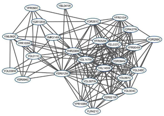
PROCODE Cluster with 28 proteins.
Fig. 2.
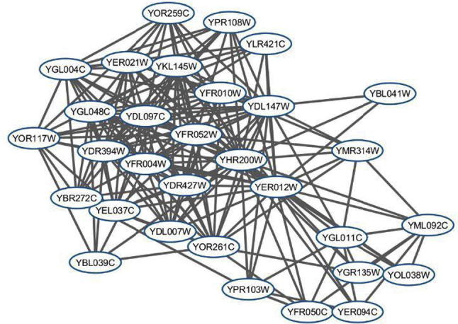
PROCODE Cluster with 31 proteins.
We also compared the clusters found by MCL algorithm with the protein complexes found by PROCODE. MCL partitioned the PPI network of DIP data into 1246 clusters. Among these, only 277 clusters are identified as having significant Biological Process annotations, 216 having Molecular Function annotation and 226 are having Cellular Component annotations. This implies that, almost 900 to 1000 of the clusters were not significant. Whereas, out of 153 protein complexes detected by PROCODE there exist 147 protein complexes having significant gene ontology annotations. In spite of the fact that MCL is capable of producing more clusters, the number of significant clusters and the biological significance within the clusters are low.
5.2.2. Size distribution analysis and evaluation of predicted complexes
In this section, we report the distribution of the sizes of predicted complexes for different methods. In Fig. 5, Fig. 6, Fig. 7, comparative graphs are plotted considering the predicted complexes of PROCODE, MCODE, COACH and ClusterONE. On close observation on the results, we found that for DIP data, largest complex is predicted by MCODE with size 107 while number of predicted complexes is minimum in MCODE (71). For DIP data, COACH has predicted the maximum number of complexes (730) and the largest complex among them is of size 85. ClusterONE predicted 342 complexes and the largest among them is of size 23, whereas, PROCODE predicted 153 complexes and the size of the largest complex is 31. Similarly, for Krogan data, maximum number of complexes is predicted by COACH, but largest complex is predicted by PROCODE. Again, for MIPS data, largest complex is given by COACH, but maximum number of predicted complexes is given by ClusterONE.
Fig. 5.

Distribution of the Sizes of the Predicted Complexes for DIP data.
Fig. 6.

Distribution of the Sizes of the Predicted Complexes for Krogan data.
Fig. 7.

Distribution of the Sizes of the Predicted Complexes for MIPS data.
In Table 2, Table 3, we have shown a detailed comparison among various competing protein complex detection algorithms over DIP data and Krogan data, respectively. For each method, #complexes denotes the total number of predicted complexes, #covered proteins denotes the number of proteins included in the predicted complexes, is the number of predicted complexes which match with at least one actual complex from the benchmark set and is the number of actual complexes that match with at least one predicted complex. For example, in Table 2, MCODE predicted 71 complexes, out of which 32 complexes matched with at least one actual complex and 261 actual complexes from the benchmark set matched with at least one predicted complex. There are 4934 proteins in the DIP PPI network, out of which 732 proteins are included in the 71 predicted complexes. Whereas, PROCODE predicted 153 complexes covering 699 proteins out of 4934 proteins in DIP.
Table 2.
Performance evaluation over DIP data.
| Algorithms | MCODE | MCL | RNSC | COACH | CORE | CFinder | DPClus | ClusterONE | PROCODE |
|---|---|---|---|---|---|---|---|---|---|
| #Complexes | 71 | 1246 | 2435 | 730 | 1722 | 245 | 1143 | 342 | 153 |
| #Covered proteins | 732 | 4930 | 4930 | 1891 | 3777 | 2008 | 2987 | 1366 | 699 |
| 32 | 212 | 234 | 255 | 221 | 84 | 193 | 99 | 96 | |
| 261 | 256 | 289 | 375 | 256 | 111 | 274 | 303 | 257 |
Table 3.
Performance evaluation over Krogan et al.’s data.
| Algorithms | MCODE | MCL | RNSC | COACH | CORE | CFinder | DPClus | ClusterONE | PROCODE |
|---|---|---|---|---|---|---|---|---|---|
| #Complexes | 75 | 834 | 1890 | 345 | 1232 | 122 | 689 | 239 | 130 |
| #Covered proteins | 550 | 3581 | 3581 | 1070 | 2665 | 1578 | 1996 | 1062 | 659 |
| 45 | 147 | 245 | 186 | 201 | 45 | 167 | 102 | 85 | |
| 202 | 197 | 283 | 276 | 229 | 63 | 241 | 270 | 230 |
A comparative analysis of PROCODE with MCODE, COACH and ClusterONE in terms of Precision, Recall and F-measure is given in Table 4.
Table 4.
Performance evaluation over MIPS data.
| Algorithms | MCODE | COACH | ClusterONE | PROCODE |
|---|---|---|---|---|
| #Complexes | 162 | 472 | 691 | 98 |
| #Covered proteins | 852 | 1270 | 2396 | 431 |
| 32 | 170 | 125 | 59 | |
| 295 | 321 | 376 | 192 | |
| Precision | 0.1975 | 0.3601 | 0.1808 | 0.6020 |
| Recall | 0.6892 | 0.75 | 0.8785 | 0.4485 |
| F-measure | 0.3070 | 0.4865 | 0.2998 | 0.5140 |
In Fig. 4 we can see that PROCODE has outperformed most of the competing algorithms taken under consideration by showing greater precision and F-measure values. We can also notice that PROCODE algorithm has performed well compared to most of the competing algorithms using Krogan et al.’s data as shown in Fig. 3.
Fig. 4.

Performance comparison in terms of Precision, Recall and F-measure for DIP data.
Fig. 3.

Performance comparison in terms of Precision, Recall and F-measure for Krogan et al.’s data.
In order to substantiate the findings we have included the Sensitivity, PPV and Accuracy measures. These are commonly used metrics to assess the performance of protein complex detection algorithms. Ji et al. [32], Li et al. [33] are among those who have used these metrics for performance evaluation. The results are shown in Fig. 8, Fig. 9, Fig. 10 for the datasets DIP, MIPS and Krogan respectively. Nevertheless, we should realize that all these metrics used to evaluate the performance of the mining algorithms are certainly not the absolute measures, they all have their pros and cons.
Fig. 8.

Comparison of PROCODE and its counterparts over DIP data.
Fig. 9.

Comparison of PROCODE and its counterparts over MIPS data.
Fig. 10.

Comparison of PROCODE and its counterparts over Korogan’s data.
We have also calculated the overall Cluster Score for DIP data and MIPS datasets and found 0.967 and 0.99 respectively. We have calculated the co-localization score for complexes using DIP data. We found 5 complexes with co-localization value 1.0 and the average co-localization value is found to be 0.5499 whereas for the same dataset COACH gives a co-localization score of value 0.75. Co-localization score of ClusterONE for DIP dataset is 0.62 and co-localization score of MCODE for the same dataset is 0.48.
5.3. Results on human data
Various works on protein complex detection methods usually use data from the yeast S. Cerevisiae for their experimental evaluation due to the fact that yeast has been studied thoroughly during the past decades and yeast data is stored and made available in various public databases to be used by researchers worldwide. Nowadays, researchers are also trying to use Homo sapien data to evaluate their methods. However, working with Homo sapien data is very challenging due to the fact that human PPI data is noisy, huge size of the PPI data, more number of smaller complexes, some of the complex sizes are also huge, proteins existing in multiple complexes and having overlapping functions as well as nomenclature problem such as different UNIPROT human IDs mapping to the same protein [42]. In this paper, we take it as a challenge to evaluate PROCODE based on human data. We used the preprocessed Human PPI network data from [43] having a total of 37,437 number of PPI interactions. The benchmark complex set of CORUM [25] was used as the gold standard containing 1843 human complexes. In the Human PPI network, PROCODE achieved a precision, recall and f-measure of 0.242, 0.158 and 0.191, when matched with the benchmark complexes of the CORUM data as shown in Fig. 11. The other counterpart methods MCODE, COACH, ClusterONE and WEC [43] achieved f-measure values of 0.077, 0.197, 0.163 and 0.19. We observe from the Fig. 11 that PROCODE has achieved the second best performance after COACH in terms of f-measure with a value of 0.191. We can say that PROCODE’s performance is almost at par with COACH. Therefore, we can conclude that PROCODE predicts complexes quite well.
Fig. 11.

The f-measure value obtained by MCODE, COACH, ClusterONE, WEC and PROCODE on the human network data.
We also computed the sensitivity, PPV and accuracy scores of PROCODE and its counterparts and the results are shown in Fig. 12. PROCODE obtained a sensitivity score of 0.51, PPV score of 0.041 and accuracy score of 0.144. PROCODE had the highest sensitivity score indicating a good prediction coverage of the predicted proteins in the real complexes. ClusterONE had the highest PPV and accuracy values with scores of 0.154 and 0.27 respectively.
Fig. 12.

TheSensitivity, PPV and Accuracyscores obtained by MCODE, COACH, ClusterONE, PROCODE and WEC on the human network data.
5.4. Conclusion and discussion
Our proposed technique, PROCODE is designed to detect the protein complexes from the PPI network by identifying the dense and possibly overlapping regions. After performing various comparative analysis on PROCODE along with other competing algorithms, we conclude that although PROCODE could not outperform all the algorithms, it stands at par with most of the compared algorithms in terms of p-value, Precision, Recall, F-measure, Sensitivity, PPV and Accuracy. It has also shown satisfactory results while considering Gene Ontology Annotation with MCL, MCODE and PCA-rdr. Although Sensitivity, PPV and Accuracy metrics have their own limitations, we can still have some idea about the algorithm’s performance by applying these metrics. In case of PROCODE, it has performed best for the MIPS dataset and for Krogan and DIP dataset it’s performance was average. The p-values obtained for the predicted complexes of PROCODE are quite low which generally indicates that the predicted complexes has high statistical significance (Refer to supplementary material). The proportion of significant complexes over the total number of predicted complexes of PROCODE is 11.5%, 26.71% and 2.85% higher than MCODE, ClusterONE and COACH respectively (Table 1). This may indicate that the collective occurrence of proteins in all the predicted complexes of PROCODE retains better biological significance than the compared ones. Nevertheless, COACH has covered much larger number of proteins than PROCODE, MCODE and ClusterONE (for DIP data) and managed to predict a comparatively larger proportion of the complexes as significant. In the human PPI network also our method performs relatively well in term of predictive capacity having an f-measure score of 0.191 lesser than Coach by a small margin and better than WEC. In terms of biological relevance, the p-values obtained are very good with the lowest p-value of 2.12E-113 for the GO term GO:0007169 (refer to Supplemetary material).
Many algorithms have been proposed and used to detect protein complexes. But it is still difficult to accurately and efficiently predict all biologically relevant protein complexes across different datasets. It should also be mentioned that to make it more meaningful and useful, the protein complex detection from PPI network should also give much emphasis on graph mining techniques. The success of these approaches also largely depends on the advancement of the experimental techniques adopted by the biologists to provide reliable and rich biological datasets for computation. Hence, when computer scientists and biologists will work in collaboration with each other, it would be much easier for the computer scientists, with added knowledge provided by the biologists, to exploit the protein interaction data and to provide efficient and robust ways for mining new knowledge from PPI data.
An executable of PROCODE is now available at (http://agnigarh.tezu.ernet.in/∼dkb/procode/index.html). We aim to make available both the source codes/executable in public code repository in future.
Footnotes
Peer review under responsibility of Academy of Scientific Research & Technology.
Supplementary data associated with this article can be found, in the online version, at https://doi.org/10.1016/j.jgeb.2017.10.010.
Contributor Information
Rosy Sarmah, Email: rosy8@tezu.ernet.in.
Dhruba K. Bhattacharyya, Email: dkb@tezu.ernet.in.
Supplementary material
References
- 1.Alberts Bruce. The cell as a collection of protein machines: preparing the next generation of molecular biologists. Cell. 1998;92(3):291–294. doi: 10.1016/s0092-8674(00)80922-8. [DOI] [PubMed] [Google Scholar]
- 2.Gavin Anne-Claude. Proteome survey reveals modularity of the yeast cell machinery. Nature. 2006;440(7084):631–636. doi: 10.1038/nature04532. [DOI] [PubMed] [Google Scholar]
- 3.Pizzuti Clara, Rombo Simona E. Algorithms and tools for proteinprotein interaction networks clustering, with a special focus on population-based stochastic methods. Bioinformatics. 2014;30(10):1343–1352. doi: 10.1093/bioinformatics/btu034. [DOI] [PubMed] [Google Scholar]
- 4.Uetz Peter. A comprehensive analysis of proteinprotein interactions in Saccharomyces cerevisiae. Nature. 2000;403(6770):623–627. doi: 10.1038/35001009. [DOI] [PubMed] [Google Scholar]
- 5.Ito Takashi. A comprehensive two-hybrid analysis to explore the yeast protein interactome. Proc Natl Acad Sci. 2001;98(8):4569–4574. doi: 10.1073/pnas.061034498. [DOI] [PMC free article] [PubMed] [Google Scholar]
- 6.Spirin Victor, Mirny Leonid A. Protein complexes and functional modules in molecular networks. Proc Natl Acad Sci. 2003;100(21):12123–12128. doi: 10.1073/pnas.2032324100. [DOI] [PMC free article] [PubMed] [Google Scholar]
- 7.Hartwell Leland H. From molecular to modular cell biology. Nature. 1999;402:C47–C52. doi: 10.1038/35011540. [DOI] [PubMed] [Google Scholar]
- 8.Liu Guimei, Wong Limsoon, Chua Hon Nian. Complex discovery from weighted PPI networks. Bioinformatics. 2009;25(15):1891–1897. doi: 10.1093/bioinformatics/btp311. [DOI] [PubMed] [Google Scholar]
- 9.Chua Hon Nian. Using indirect protein protein interactions for protein complex prediction. J Bioinform Comput Biol. 2008;6(03):435–466. doi: 10.1142/s0219720008003497. [DOI] [PubMed] [Google Scholar]
- 10.Li Xiao-Li. Interaction graph mining for protein complexes using local clique merging. Genome Inform. 2005;16(2):260–269. [PubMed] [Google Scholar]
- 11.Altaf-Ul-Amin Md. Development and implementation of an algorithm for detection of protein complexes in large interaction networks. BMC Bioinform. 2006;7(1):207. doi: 10.1186/1471-2105-7-207. [DOI] [PMC free article] [PubMed] [Google Scholar]
- 12.Wu Min. A core-attachment based method to detect protein complexes in PPI networks. BMC Bioinform. 2009;10(1):169. doi: 10.1186/1471-2105-10-169. [DOI] [PMC free article] [PubMed] [Google Scholar]
- 13.Feng Jianxing, Jiang Rui, Jiang Tao. A max-flow-based approach to the identification of protein complexes using protein interaction and microarray data. IEEE/ACM Trans Comput Biol Bioinform. 2011;8(3):621–634. doi: 10.1109/TCBB.2010.78. [DOI] [PubMed] [Google Scholar]
- 14.Maraziotis Ioannis A., Dimitrakopoulou Konstantina, Bezerianos Anastasios. Growing functional modules from a seed protein via integration of protein interaction and gene expression data. Bmc Bioinform. 2007;8(1):408. doi: 10.1186/1471-2105-8-408. [DOI] [PMC free article] [PubMed] [Google Scholar]
- 15.King Andrew D., PrÅulj N., Jurisica Igor. Protein complex prediction via cost-based clustering. Bioinformatics. 2004;20(17):3013–3020. doi: 10.1093/bioinformatics/bth351. [DOI] [PubMed] [Google Scholar]
- 16.Bader Gary D., Hogue Christopher W.V. An automated method for finding molecular complexes in large protein interaction networks. BMC Bioinform. 2003;4(1):2. doi: 10.1186/1471-2105-4-2. [DOI] [PMC free article] [PubMed] [Google Scholar]
- 17.Dongen Van, Marinus Stijn. Graph clustering by flow simulation; 2001.
- 18.Leung Henry C.M. Predicting protein complexes from PPI data: a core-attachment approach. J Computat Biol. 2009;16(2):133–144. doi: 10.1089/cmb.2008.01TT. [DOI] [PubMed] [Google Scholar]
- 19.Adamcsek Balzs. CFinder: locating cliques and overlapping modules in biological networks. Bioinformatics. 2006;22(8):1021–1023. doi: 10.1093/bioinformatics/btl039. [DOI] [PubMed] [Google Scholar]
- 20.Xenarios Ioannis. DIP, the Database of Interacting Proteins: a research tool for studying cellular networks of protein interactions. Nucl Acids Res. 2002;30(1):303–305. doi: 10.1093/nar/30.1.303. [DOI] [PMC free article] [PubMed] [Google Scholar]
- 21.Mewes Hans-Werner. MIPS: analysis and annotation of proteins from whole genomes. Nucl Acids Res. 2004;32(suppl 1):D41–D44. doi: 10.1093/nar/gkh092. [DOI] [PMC free article] [PubMed] [Google Scholar]
- 22.Krogan Nevan J. Global landscape of protein complexes in the yeast Saccharomyces cerevisiae. Nature. 2006;440(7084):637–643. doi: 10.1038/nature04670. [DOI] [PubMed] [Google Scholar]
- 23.Nymark P., Lindholm P.M., Korpela M.V., Lahti L. Gene expression profiles in asbestos-exposed epithelial and mesothelial lung cell lines. BMC Genom. 2007;1(1) doi: 10.1186/1471-2164-8-62. [DOI] [PMC free article] [PubMed] [Google Scholar]
- 24.Wang Shuliang, Wu Fang. Detecting overlapping protein complexes in PPI networks based on robustness. Prot Sci. 2013;11(Suppl 1):S18. doi: 10.1186/1477-5956-11-S1-S18. [DOI] [PMC free article] [PubMed] [Google Scholar]
- 25.Ruepp A., Waegele B., Lechner M., Brauner B., Dunger-Kaltenbach I., Fobo G. CORUM: the comprehensive resource of mammalian protein complexes. Nucl Acids Res. 2010;38:D497–D501. doi: 10.1093/nar/gkp914. [DOI] [PMC free article] [PubMed] [Google Scholar]
- 26.Jansen Ronald, Gerstein Mark. Analyzing protein function on a genomic scale: the importance of gold-standard positives and negatives for network prediction. Curr Opin Microbiol. 2004;7(5):535–545. doi: 10.1016/j.mib.2004.08.012. [DOI] [PubMed] [Google Scholar]
- 27.Nepusz Tams, Yu Haiyuan, Paccanaro Alberto. Detecting overlapping protein complexes in protein-protein interaction networks. Nat Methods. 2012;9(5):471–472. doi: 10.1038/nmeth.1938. [DOI] [PMC free article] [PubMed] [Google Scholar]
- 28.Jansen Ronald. A Bayesian networks approach for predicting protein-protein interactions from genomic data. Science. 2003;302(5644):449–453. doi: 10.1126/science.1087361. [DOI] [PubMed] [Google Scholar]
- 29.Goodman Steven N. Toward evidence-based medical statistics. 1: the P value fallacy. Annals Internal Med. 1999;130(12):995–1004. doi: 10.7326/0003-4819-130-12-199906150-00008. [DOI] [PubMed] [Google Scholar]
- 30.Goodman Steven N. Toward evidence-based medical statistics. 2: the Bayes factor. Annals Internal Med. 1999;130(12):1005–1013. doi: 10.7326/0003-4819-130-12-199906150-00019. [DOI] [PubMed] [Google Scholar]
- 31.Asur Sitaram, Ucar Duygu, Parthasarathy Srinivasan. An ensemble framework for clustering proteinprotein interaction networks. Bioinformatics. 2007;23(13):i29–i40. doi: 10.1093/bioinformatics/btm212. [DOI] [PubMed] [Google Scholar]
- 32.Ji Junzhong. Survey: functional module detection from protein-protein interaction networks. IEEE Trans Knowl Data Eng. 2014;26(2):261–277. [Google Scholar]
- 33.Li Xiaoli. Computational approaches for detecting protein complexes from protein interaction networks: a survey. BMC Genom. 2010;11(Suppl 1):S3. doi: 10.1186/1471-2164-11-S1-S3. [DOI] [PMC free article] [PubMed] [Google Scholar]
- 34.Maraziotis Ioannis A., Dimitrakopoulou Konstantina, Bezerianos Anastasios. Growing functional modules from a seed protein via integration of protein interaction and gene expression data. Bmc Bioinform. 2007;8(1):408. doi: 10.1186/1471-2105-8-408. [DOI] [PMC free article] [PubMed] [Google Scholar]
- 35.Aloy Patrick. Structure-based assembly of protein complexes in yeast. Science. 2004;303(5666):2026–2029. doi: 10.1126/science.1092645. [DOI] [PubMed] [Google Scholar]
- 36.Dwight Selina S. Saccharomyces Genome Database (SGD) provides secondary gene annotation using the Gene Ontology (GO) Nucl Acids Res. 2002;30(1):69–72. doi: 10.1093/nar/30.1.69. [DOI] [PMC free article] [PubMed] [Google Scholar]
- 37.Wu Min. Benchmarking human protein complexes to investigate drug-related systems and evaluate predicted protein complexes. PloS One. 2013;8(2):e53197. doi: 10.1371/journal.pone.0053197. [DOI] [PMC free article] [PubMed] [Google Scholar]
- 38.Berriz Gabriel F. Next generation software for functional trend analysis. Bioinformatics. 2009;25(22):3043–3044. doi: 10.1093/bioinformatics/btp498. [DOI] [PMC free article] [PubMed] [Google Scholar]
- 39.Berriz Gabriel F. Characterizing gene sets with FuncAssociate. Bioinformatics. 2003;19(18):2502–2504. doi: 10.1093/bioinformatics/btg363. [DOI] [PubMed] [Google Scholar]
- 40.Brohee Sylvain, Helden Jacques Van. Evaluation of clustering algorithms for protein-protein interaction networks. BMC Bioinform. 2006;7(1):488. doi: 10.1186/1471-2105-7-488. [DOI] [PMC free article] [PubMed] [Google Scholar]
- 41.Friedel Caroline C., Krumsiek Jan, Zimmer Ralf. Springer; Berlin Heidelberg: 2008. Bootstrapping the interactome: unsupervised identification of protein complexes in yeast. Research in Computational Molecular Biology. [DOI] [PubMed] [Google Scholar]
- 42.Liu Q., Song J., Li J. Using contrast patterns between true complexes and random subgraphs in PPI networks to predict unknown protein complexes. Scient Rep. 2016;6 doi: 10.1038/srep21223. [DOI] [PMC free article] [PubMed] [Google Scholar]
- 43.Keretsua S., Sarmah R. Weighted edge based clustering to identify protein complexes in proteinprotein interaction networks incorporating gene expression profile. Comput Biol Chem. 2016;65:69–79. doi: 10.1016/j.compbiolchem.2016.10.001. [DOI] [PubMed] [Google Scholar]
Associated Data
This section collects any data citations, data availability statements, or supplementary materials included in this article.