Instability-driven oscillations of elastic microfilaments

Abstract

Cilia and flagella are highly conserved slender organelles that exhibit a variety of rhythmic beating patterns from non-planar cone-like motions to planar wave-like deformations. Although their internal structure, composed of a microtubule-based axoneme driven by dynein motors, is known, the mechanism responsible for these beating patterns remains elusive. Existing theories suggest that the dynein activity is dynamically regulated, via a geometric feedback from the cilium’s mechanical deformation to the dynein force. An alternative, open-loop mechanism based on a ‘flutter’ instability was recently proven to lead to planar oscillations of elastic filaments under follower forces. Here, we show that an elastic filament in viscous fluid, clamped at one end and acted on by an external distribution of compressive axial forces, exhibits a Hopf bifurcation that leads to non-planar spinning of the buckled filament at a locked curvature. We also show the existence of a second bifurcation, at larger force values, that induces a transition from non-planar spinning to planar wave-like oscillations. We elucidate the nature of these instabilities using a combination of nonlinear numerical analysis, linear stability theory and low-order bead–spring models. Our results show that, away from the transition thresholds, these beating patterns are robust to perturbations in the distribution of axial forces and in the filament configuration. These findings support the theory that an open-loop, instability-driven mechanism could explain both the sustained oscillations and the wide variety of periodic beating patterns observed in cilia and flagella.

1. Introduction

Cilia and flagella are microscopic hair-like organelles found in many eukaryotic cells, from single-celled protozoa to mammalian epithelial surfaces. They are driven into oscillatory motion by an intricate internal structure, referred to as the central axoneme, composed of microtubule doublets and dynein molecular motors (figure 1). Despite the highly conserved structure of the central axoneme across eukaryotic cells, cilia and flagella of different cells exhibit wildly different beating patterns, from non-planar cone-like motions to planar wave-like deformations [6,7]. The mechanisms that regulate the activity of the dynein motors, causing them to produce oscillatory motions, remain elusive, and even less is known about the mechanisms leading to this diversity in beating patterns [8–11]. Several theoretical studies support the hypothesis that dynein motors are regulated by a geometric feedback from mechanical deformations to molecular activity [1,3,12,13].

Figure 1.

Internal structure of a cilium/flagellum. (a) Cross-section of a typical cilium/flagellum. A bridge exists between two of the doublets, thus the dynein motors are usually separated into principal (P) and reverse (R) sides. Feedback control hypotheses [1–3] are based on the theory that P,R sides are activated in alternating fashion owing to kinematic constraints. But even when both sides are activated in roughly equal amounts, a flutter instability could drive the cilium into oscillations [4,5]. (b,c) In both theories, internal force couples (f_D) generated by dynein motors walking towards the minus (−) end of microtubule doublets effectively apply an ‘external force’ on the centreline. This external loading is explicitly coupled with the kinematics of the centreline. (Online version in colour.)

Brokaw was the first to show that delayed feedback from curvature to dynein activity could lead to oscillations [1,14–16]. Hines & Blum [17] developed detailed models of elastic filaments that generate sustained oscillations with curvature feedback control. Murase, Jülicher and others demonstrated the existence of oscillatory modes in sliding-control models [18–21]. Lindemann proposed a ‘geometric clutch’ hypothesis, where the dynein activity changes as a function of the spacing between doublet pairs, leading to axoneme oscillations [2,22–24]. A comparison of these various feedback mechanisms with experimental observations seems to favour the hypothesis of regulation by curvature feedback control [3].

Although these feedback models are appealing, Bayly & Dutcher [4] argued convincingly that evidence supporting the hypothesis that dynein regulation is required for bending oscillations remains circumstantial. They then proposed an alternative mechanism that does not require regulation of dynein activity to generate oscillatory motions [4,5]. The mechanism relies on a dynamic buckling instability induced by the internal dynein forces, which apply axial stresses to the axoneme as it deforms. This instability is reminiscent of the classic Euler buckling instability, but, instead of the familiar static instability under fixed forces, these follower forces lead to a dynamic buckling instability, known as a ‘flutter’ instability in aeroelasticity [25] or, more informally, as the ‘garden hose’ instability [26,27]. To demonstrate that this dynamic instability could lead to sustained oscillations in cilia and flagella, Bayly and Dutcher used elaborate models of the axoneme, including finite-element analysis and a model of two filaments, representing pairs of microtubule doublets connected via passive elements of elastic spring and viscous damping. Han & Peskin [28] also proposed an elaborate model of the axoneme structure that leads to sustained oscillations via a dynamic instability. De Canio et al. [29] explored the concept of instability-driven oscillations in the context of a simpler model, consisting of a single microfilament, confined to planar motion, clamped at one end and acted on by an external follower force at the free end.

Mathematical models, whether in support of curvature-feedback control or instability-driven oscillations, should be regarded as an abstraction of the intricate internal structure of cilia and flagella (figure 1). Representations of the details of this structure require several assumptions in terms of model parameters (e.g. stiffness and damping coefficients for inter-doublet links), internal geometric constraints and dynein activation laws [4,5,24,28]. Such a level of detail is often ignored in favour of analytical rod models of the cilium centreline, where the internal dynein forces can be nominally treated as a distribution of ‘external’ forces or moments along the centreline. For example, in [30] and references therein, the internal forces are modelled in terms of a distribution of external moments only along the filament centreline (note that one could rewrite these moments in terms of tangential and normal forces). In [3,21], the cilium is reduced first to two coupled filaments, then to an effective set of equations governing the dynamics of the centreline of these two filaments subject to a distribution of active tangential and normal forces; see [3, eqn (12)]. Although it is clear from a homogenization approach that such centreline representation should exist, deriving the equations of motion and effective forces acting on the centreline from more elaborate, coupled, multi-filament models of the axoneme structure is generally a difficult task; it typically leads to forces that are explicitly coupled to the centreline curvature (e.g. as in [3, eqn (12)], [31, eqn (A18–19)]). This coupling could be essential to explain some of the seemingly non-local effects observed in flagellar mechanics due to local deformations [32–35]. In the model of [4], the cilium is represented by two coupled microfilaments subject to a distribution of internal forces; the interesting result is that, even when the internal forces are balanced such that they effectively produce no moments on the cilium, oscillations ensue as a result of a flutter instability. A derivation of a centreline model based on the two-filament model of [4] (results in preparation) would allow rigorous comparisons with other centreline models (e.g. [3,31]). Here, for the sake of simplicity and clarity, we analyse the case of a single filament with distributed axial forces of constant magnitude, as a useful, albeit idealized, analogue for the more complicated centreline force profiles that arise in flagellar mechanics.

More specifically, we consider an elastic microfilament in a viscous fluid, clamped at one end and acted upon by a distribution of axial forces (figure 2). Unlike [29], the filament is free to undergo three-dimensional (3D) motions. To investigate the filament deformations in 3D, we adapt the numerical framework advanced by Bergou et al. [36] and Gazzola et al. [37], as well as a combination of linear stability theory and a low-order bead–spring model. We show that the filament exhibits a Hopf bifurcation that leads to sustained oscillations, consistent with [29]. However, unlike [29], the filament undergoes non-planar spinning motions, reminiscent of the cone-like beating motion of cilia, and microtubule streaming motion studied in [38]. Importantly, at larger axial forces, we show the existence of another bifurcation, not reported in [29], that causes the filament to transition from 3D spinning to planar wave-like deformations. We investigate the transition from 3D spinning to two-dimensional (2D) flapping under various axial force profiles and in the bead–spring model. We conclude by commenting on the significance of these results for biological cilia and flagella.

Figure 2.

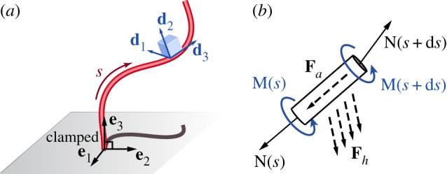
The microfilament model. (a) Schematic of a flexible filament clamped at one end and free at its tip. The filament position is defined by r(s, t), with 0 < s < L being the arc-length. Its configuration is determined by the orientation of the material frame {d₁, d₂, d₃}, with d₃ = ∂r/∂s. (b) The forces and moments that apply on an infinitesimal filament element ds. See text for notation. (Online version in colour.)

2. Microfilament model

Consider an inextensible elastic filament of length L and circular cross-section of radius a, clamped at its base normally to a fixed plane (x, y) (figure 2a). Let {e₁, e₂, e₃} be an inertial frame, attached at the filament base, such that {e₁, e₂} span the (x, y)-plane. The centreline of the filament is described by the vector r(s, t) where s is arc-length and t is time. The local orientation of the filament is described by an orthonormal material frame {d₁, d₂, d₃}, with d₃ = ∂r/∂s = t the tangential unit vector. The change of {d₁, d₂, d₃} along the filament, at some time t, is given by

$$\frac{\mathrm{\partial }{\mathbf{d}}_j}{\mathrm{\partial }s}=\kappa \times {\mathbf{d}}_j,\hspace{0.17em}j=1,\hspace{0.17em}2,\hspace{0.17em}3,$$ 2.1

where κ is a generalized curvature vector recording the infinitesimal change in orientation along the filament (e.g. [39]). Specifically, given the rotation matrix Q(s, t) that maps vectors expressed in the inertial frame to their counterparts in the filament material frame, κ is the vector representation, in the material frame, of the skew-symmetric matrix ${\mathit{\kappa }}^{\times }=\mathbf{Q}{({\mathbf{Q}}^{\prime })}^{\mathsf{T}}$, where the prime denotes differentiation with respect to s and ${()}^{\mathsf{T}}$ is the transpose operator.

The balance of forces and moments on a cross-section of the filament are given by the Kirchhoff equations [40], subject to the clamped–free boundary conditions

$$\frac{\mathrm{\partial }\mathbf{N}}{\mathrm{\partial }s}+{\mathbf{f}}_{\mathrm{h}}+{\mathbf{f}}_{\mathrm{a}}=0\text{and}\frac{\mathrm{\partial }\mathbf{M}}{\mathrm{\partial }s}+\mathbf{t}\times \mathbf{N}=0.$$ 2.2

Here, N and M are the internal elastic force and bending moment, respectively, f_h is the hydrodynamic force per unit length, and f_a is the applied force per unit length. Taking the cross-product of the tangent vector t with the balance of moments in (2.2), the internal elastic force can be readily rewritten as

$$\mathbf{N}=\mathbf{t}\times \left(\frac{\mathrm{\partial }\mathbf{M}}{\mathrm{\partial }s}\right)+\mathit{\Lambda }\mathbf{t},$$ 2.3

where $\mathit{\Lambda }=\mathbf{N}\cdot \mathbf{t}$ is a Lagrange multiplier that enforces the inextensibility constraint $\mathbf{t}\cdot \mathbf{t}=1$. Physically, Λ represents the axial tension along the filament.

We take advantage of the small aspect ratio of the filament (a/L ≪ 1) and use the resistive force theory that linearly relates f_h to the instantaneous distribution of velocities $\mathbf{v}=\dot{\mathbf{r}}$ along the filament centreline, where the dot denotes differentiation with respect to time t. Specifically, ${\mathbf{f}}_{\mathrm{h}}=-[{\zeta }_{\parallel }\mathbf{t}\mathbf{t}+{\zeta }_{\perp }({\mathbf{d}}_1{\mathbf{d}}_1+{\mathbf{d}}_2{\mathbf{d}}_2)]\mathbf{v}$ is related to v via the anisotropic drag coefficients ζ_⊥ = 4πμ/ln(L/a) and ${\zeta }_{\parallel }={\zeta }_{\perp }/\gamma$, with γ = 2 (e.g. [41]); equivalently,

$${\mathbf{f}}_{\mathrm{h}}=-{\zeta }_{\perp }[\mathbf{I}-\frac{\gamma -1}{\gamma }\mathbf{t}\mathbf{t}]\mathbf{v}.$$ 2.4

To arrive at (2.4), we introduce the identity matrix I = d₁d₁ + d₂d₂ + tt.

The force per unit length f_a emulates the effect of the dynein activity, which we assume induces a compressive force density f_a = −f_at along the centreline of the filament. This model is reminiscent of the models presented in [29], with the distinction that the distribution of the force density may vary along the filament, f_a = f_a(s), such that the total compressive force is given by $F_{\mathrm{a}}={\int }_0^L{f}_{\mathrm{a}}\hspace{0.17em}\text{d}s$. Non-tangential forces as well as bending and twist moments are ignored.

We consider a linear constitutive relation between the internal elastic moment M and κ. For an axisymmetric filament with circular cross-section of area A and Young’s modulus E, this linear relation simplifies to M = Bκ, where $\mathbf{B}=B\hspace{0.17em}\mathrm{diag}(1,1,2)$ is the bending rigidity tensor, expressed in the filament material frame, and B = EA² is the stiffness coefficient. It is worth noting that the energy needed to produce twist is of order L/a larger than that to produce bending; therefore, we not only ignore the twist moments due to dynein activity, but also the tangential component of the internal moment, that is, we set $\mathbf{M}\cdot \mathbf{t}=0$, which yields no twist of the filament [30].

In the absence of twist, the generalized curvature κ can be expressed as κ = k₁d₁ + k₂d₂. Here, k₁(s, t) and k₂(s, t) are scalar curvature functions, related to the curvature κ(s, t) and torsion τ(s, t) in the Frenet–Serret formulation, such that $\kappa =\sqrt{k_1^2+k_2^2}$ and τ = ∂[tan⁻¹(k₂/k₁)]/∂s. It is important to distinguish here between twist and torsion. It is also worth noting that the Frenet–Serret frame (n, b, t), where n and b are the normal and binormal unit vectors, is not a material frame. In particular, {d₁, d₂, d₃ ≡ t} is related to (n, b, t) through a rigid rotation about the t-direction by an angle equal to tan⁻¹(k₂/k₁).

The dimensional parameters and characteristic scales relevant for cilia and flagella are summarized in table 1. Here, we rewrite the system of equations in non-dimensional form using the filament length L as the characteristic length scale and T = L⁴ζ_⊥/B as the characteristic time scale. The intrinsic time scale T arises from balancing the elastic and hydrodynamic forces. The model admits a second time scale T_a = ζ_⊥L²/F_a that arises from balancing the total applied force with the hydrodynamic force. The ratio of the two time scales T/T_a = F_aL²/B is equivalent to a dimensionless force, which we use in §5 as the main parameter to study the filament behaviour. The non-dimensional system of equations is characterized by the drag anisotropy parameter $\gamma ={\zeta }_{\perp }/{\zeta }_{\parallel }=2$, and the parameters that describe the distribution of axial forces along the filament centreline, giving rise to the non-dimensional force F_aL²/B. In the following, we consider all variables and parameters to be non-dimensional.

Table 1.

Characteristic scales of cilia and flagella.

parameter	symbol	dimensional value
bending rigidity	B	$800\hspace{0.17em}\hspace{0.17em}\text{pN}\cdot \mu {\text{m}}^2$ [42]
filament length	L	20 µm
fluid viscosity	$\mu \approx {\mu }_{\mathrm{water},{20}^{\circ }}$	${10}^{-3}\hspace{0.17em}\text{Pa}\cdot \text{s}$
time scale	L4ζ⊥/B	0.546 s
frequency scale	B/(L4ζ⊥)	1.83 Hz
force scale	B/L2	2 pN
force density	B/L3	$0.1\hspace{0.17em}\hspace{0.17em}\text{pN}\cdot \mu {\text{m}}^{-1}$
slenderness ratio	a/L	1/100
normal drag	${\zeta }_{\perp }=\frac{4\pi \mu }{\ln (L/a)}$	$2.73\times {10}^{-3}\hspace{0.17em}\text{Pa}\cdot \text{s}$

3. Numerical method

To solve for the filament dynamics in three dimensions, we numerically integrate the governing equations (2.2), together with the corresponding boundary conditions. To this end, we discretize the filament’s centreline into n + 1 vertices r₁, …, r_n+1 and n straight edges ℓ_i = r_i+1 − r_i, where i = 1, …, n, in the spirit of [36,37]. The unit tangent to edge i is defined as t _i = ℓ_i/ℓ_i, where ℓ_i = ‖ℓ_i‖. The translational velocities v₁, …, v_n+1 are assigned to vertices. The body frames {d_1,i, d_2,i, d_3,i = t_i} and the rotation matrices Q_i are naturally assigned to edges.

To obtain a discrete representation of the generalized curvature vector κ, we start from the definition of the associated skew-symmetric matrix ${\mathit{\kappa }}^{\times }=\mathbf{Q}{({\mathbf{Q}}^{\prime })}^{\mathsf{T}}$. The solution to this first-order differential equation is of the form Q(s + Δs) = exp(−κ^×Δs)Q(s), where Δs is a segment of constant curvature. Thus, writing ${\mathbf{Q}}_i=\exp (-{\mathit{\kappa }}_i^{\times }{\overline{\ell }}_i){\mathbf{Q}}_{i-1}$, we define the discrete curvature matrix as ${\mathit{\kappa }}_i^{\times }=-\ln ({\mathbf{Q}}_i{\mathbf{Q}}_{i-1}^{\mathsf{T}})/{\overline{\ell }}_i$, where ${\overline{\ell }}_i=\frac{1}{2}({\ell }_{i-1}+{\ell }_i)$ is a Voronoi integration domain from the midpoint of the previous edge to that of the next edge. Given ${\mathit{\kappa }}_i^{\times }$, we can readily evaluate κ _i and the discrete elastic moments M _i in the filament material frame.

We solve for the discrete elastic forces N_i in the material frame using (2.3). The inextensibility constraint is enforced weakly by considering a large tensile stiffness EA along the filament’s centreline. Next, we transform N_i to the inertial frame, and substitute into the balance of forces in (2.2) using the expression for the hydrodynamic force density f_h from (2.4) to get the inertial frame velocities v_i. We use standard time integrators for stiff equations (Matlab’s ode15s) to propagate the filament position r_i forward in time. To close the system, we enforce the clamped boundary condition by fixing r₁ = 0 and t₁ = e₃, while leaving the free end unconstrained. Additional details on the discretization method and numerical validation are included in the electronic supplementary material.

4. Linear stability analysis

Consider a straight filament subject to a distribution of axial forces f_a = −f_a(s)t, along the filament centreline, where f_a(s) is a general function of s. In order to assess the stability of the straight configuration, we linearize the equations of motion about the straight equilibrium and solve for the dominant eigenvalue.

To begin, we substitute (2.3) and (2.4) into the force balance in (2.2) to arrive at the vector equation

$$\dot{\mathbf{r}}=\gamma ({\mathit{\Lambda }}^{\prime }+\kappa {\kappa }^{\prime }-f_{\mathrm{a}})\mathbf{t}+(\mathit{\Lambda }{k}_2-k_2^{″})\hspace{0.17em}{\mathbf{d}}_1-(\mathit{\Lambda }{k}_1-k_1^{″})\hspace{0.17em}{\mathbf{d}}_2,$$ 4.1

where we used the fact that $\kappa =\sqrt{k_1^2+k_2^2}$. Equation (4.1) leads, upon further simplifications (see details in the electronic supplementary material), to three nonlinear scalar equations in terms of the filament tension Λ(s, t) and filament shape: curvature κ(s, t) and torsion τ(s, t). Expanding these equations about the straight equilibrium state κ = τ = 0, and linearizing with respect to κ and τ, it can be shown that vector equation (4.1) leads to two scalar equations only,

$${\mathit{\Lambda }}^{″}=f_a^{\prime }$$ 4.2

and

$${\kappa }^{⁗}-\mathit{\Lambda }{\kappa }^{″}+\gamma \dot{\kappa }=0.$$ 4.3

The third equation is trivially satisfied at the linear level. Since these equations do not depend on torsion τ(s, t), the linear analysis cannot capture 3D deformations of the filament. That is to say, in the linear regime near the straight equilibrium, the filament undergoes planar deformations. Thus, without loss of generality, we can equate the arc-length s with the z-coordinate in the inertial frame and set κ = y″, where the prime notation here denotes differentiation with respect to z. Substituting into (4.3) and integrating with respect to z twice, we arrive at the fourth-order partial differential equation

$$y^{⁗}-\mathit{\Lambda }{y}^{″}+\gamma \dot{y}=0,$$ 4.4

for the infinitesimal displacement y(z, t) in the (y, z)-plane. To close this equation, we integrate (4.2) from the free tip of the filament and define the internal traction force

$$\mathit{\Lambda }(z)={\int }_L^z{f}_{\mathrm{a}}(\tilde{z})\hspace{0.17em}\text{d}\tilde{z}.$$ 4.5

Assume the solution y(z, t) is separable in the form of y(z, t) = Y(z) e^λt, we obtain the boundary value problem

$$\begin{array}{rl}& Y^{⁗}-\mathit{\Lambda }{Y}^{″}+\lambda \gamma Y=0\\ \text{and}& Y(0)=Y^{\prime }(0)=0,Y^{″}(L)=Y^{‴}(L)=0.\end{array}\}$$ 4.6

The first two boundary conditions correspond to the clamped end and the last two to the free end. In general, the differential equation in (4.6) belongs to the class of linear differential equations with non-constant coefficients, given that Λ(z) is a function of z for a general distribution of axial forces. Therefore, depending on the form of f_a(z), this boundary value problem may not admit an analytical solution. The boundary conditions welcome the use of the free vibration modes of a clamped–free beam as test functions for a numerical solution to this boundary value problem. Namely, we expand Y(z) onto the eigenfunctions of the clamped–free linear beam equations

$$Y(z)=\sum _{i=1}^{\mathrm{\infty }}{Y}_i{\mathit{\Phi }}_i(z),$$ 4.7

where Y_i are constant coefficients and Φ_i(z) are given by

$$\begin{array}{rl}{\mathit{\Phi }}_i(z)& =\sum _{n=0}^{\mathrm{\infty }}\cosh (a_{n}z)-\cos (a_{n}z)\\ & -b_n[\sinh (a_{n}z)-\sin (a_{n}z)],\end{array}$$ 4.8

with b_n = (cos a_n + cosh a_n)/(sin a_n + sinh a_n) and a_n the nth root of the transcendental characteristic equation cos a_n cosh a_n + 1 = 0. This ‘assumed modes’ method, an extension of the classical Ritz method [43,44], was used to analyse the stability of flagella dynamics in [4,45].

Finally, we project (4.6) onto these basis functions and rewrite it in weak form as

$$\begin{array}{rl}& Y_i[{\int }_0^L{\mathit{\Phi }}_i^{″}{\mathit{\Phi }}_j^{″}\hspace{0.17em}\text{d}z-{\int }_0^L{\mathit{\Phi }}_i\mathit{\Lambda }{\mathit{\Phi }}_j^{″}\hspace{0.17em}\text{d}z+\lambda \gamma {\int }_0^L{\mathit{\Phi }}_i{\mathit{\Phi }}_j\hspace{0.17em}\text{d}z]=0.\end{array}$$ 4.9

This equation can be rewritten in matrix form as (K + C + λγM)Y = 0. Thus, the linear stability of the filament away from the straight configuration can be obtained via the eigenvalue problem K + C = −λγM. The real part of the resulting λ indicates the growth (or decay) of perturbations and the imaginary part corresponds to the frequency of a given modal shape Y_iΦ_i(z).

5. Spinning versus flapping oscillations

We first consider the set-up analysed in [29] of an elastic filament subject to a follower axial force of magnitude F_a concentrated at the distal tip of the filament (figure 3a). In [29], the filament is confined to undergo planar motions. Starting from a small perturbation away from the straight configuration, the authors identify three dynamical behaviours depending on the magnitude of the axial force F_a: (i) for small force, the filament returns monotonically to its original straight configuration, (ii) as the force value increases, the filament displays decaying oscillations back to the straight configuration, and (iii) for forces above a given threshold, the filament settles into finite-amplitude periodic deformations, which the authors referred to as planar flapping.

Figure 3.

Three-dimensional buckling. (a) Filament subject to an axial follower force of F_a, concentrated at its tip. (b) Starting from a straight configuration, the filament buckles into a locked-curvature configuration and undergoes 3D spinning motion for F_a = 75. (c) The x-, y- and z-positions of the filament distal tip point and (d) its bending energy versus time. (Online version in colour.)

Here, we start with a small non-planar perturbation away from the straight configuration and we numerically solve for the filament dynamics. In figure 3, we set F_a = 75, which lies in the planar flapping regime of [29]. Unlike the flapping behaviour reported in the latter, the filament buckles into a configuration with locked curvature and undergoes three-dimensional spinning about the z-direction, as illustrated in figure 3b. The tip displacement of the filament and its bending energy as a function of time are reported in figure 3c,d, respectively. The (x, y)-coordinates of the filament tip settle into periodic motions while the z-coordinate goes to a constant value. The filament bending energy also goes to a constant value, emphasizing that, in its buckled state, the curvature of the filament is constant (see electronic supplementary material, movie S1).

By symmetry of the geometry and material properties of the filament, planar initial perturbations lead to filament motions that remain confined to the perturbation plane. In particular, for planar initial perturbations, the filament in figure 3 undergoes 2D flapping motions, as reported in [29] (see electronic supplementary material, movie S2). However, non-planar perturbations lead to 3D spinning motions (see figure 3 and electronic supplementary material, movie S1). Taken together, these results go beyond the findings of [29] to show that, subject to non-planar perturbations, planar flapping can also be unstable.

We next examine the filament behaviour for increasing values of F_a. We observe a transition from 3D spinning to 2D wave-like oscillations, as shown in figure 4a. For F_a = 180, the filament settles into a buckled configuration with locked curvature and undergoes 3D spinning about the z-direction, whereas for F_a = 190 the filament converges in finite time to planar oscillations. The (x, y) motion of the filament tip is shown in figure 4b: the red circular trajectory corresponds to 3D spinning (F_a = 180) and the black line to 2D flapping (F_a = 190). The flapping motion occurs in an arbitrary plane, which depends on the non-planar initial perturbations. However, the frequency and amplitude of these wave-like deformations are independent of initial conditions. For 3D spinning, the z-coordinate of the filament tip and the filament bending energy go to constant values in finite time; see the decaying red lines in figure 4c,d, respectively. For the 2D flapping motion, they oscillate with constant amplitudes (black lines). It is important to distinguish between the 2D flapping motion obtained here and the planar motions of [29]. The planar motions in [29] are unstable to non-planar perturbations and are obtained as a result of confining the filament in one plane. Here, the filament dynamically converges to planar deformations, even when subject to large non-planar initial perturbations (see electronic supplementary material, movie S3). In other words, for this value of F_a, the planar motion is robust to non-planar initial perturbations.

Figure 4.

Transition from 3D spinning to 2D flapping. (a) 3D spinning motion at F_a = 180 versus 2D flapping motion at F_a = 190. (b) When projected onto the (x, y)-plane, the tip of the spinning filament traces a circular trajectory, while the trajectory of the tip of the flapping filament collapses to a fixed line. (c,d) Both the z-position of the distal tip and the total bending energy of the filament decay to constant values for spinning, but remain oscillatory for flapping. (Online version in colour.)

We plot in figure 5a the oscillation frequency of the filament as a function of F_a for the range of values considered in [29]. We compare these frequencies with the real and imaginary values of the dominant eigenvalues obtained from the linear stability analysis about the straight configuration discussed in §4. Linear stability analysis shows that the imaginary part of the dominant eigenvalue (solid black line) becomes complex at F_a ≈ 20, whereas the real part (dashed black line), associated with the rate of growth of the initial perturbation, remains negative until F_a ≈ 37.7. That is to say, the straight filament configuration is monotonically stable for F_a < 20 and stable with decaying oscillations for 20 < F_a < 37.7. The filament undergoes a Hopf bifurcation at F_a = 37.7, as the complex pair of eigenvalues crosses the imaginary axis, leading to unstable motions with growing oscillations. The linear oscillation frequencies are given by the imaginary part of the dominant eigenvalue Im[λ]/2π. The linear stability results are quantitatively consistent with those in [29].

Figure 5.

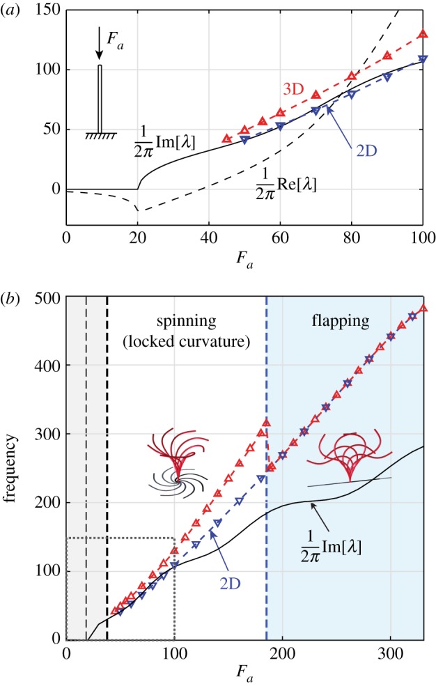
Frequency of oscillations versus linear stability analysis. (a) Real (dashed line) and imaginary (solid black line) parts of the dominant λ as a function of F_a for the range of F_a reported in [29]. A Hopf bifurcation at F_a ≈ 37.7 marks the transition from a stable straight configuration to sustained oscillations. The nonlinear oscillation frequencies are computed for non-planar perturbations (red line, up-triangle symbols) and confined planar perturbations (blue line, down-triangle symbols). Confined filaments oscillate at frequencies that are in reasonable agreement with those predicted by the linear stability analysis, while 3D spinning motions occur at higher frequencies. The relative frequency difference (1 −flapping/spinning frequency) ranges from approximately $15\text{\%}$ to approximately $20\text{\%}$. (b) Same analysis extended to a larger range of F_a—dashed box in lower left corner corresponds to the results in (a). We observe a second transition at F_a ≈ 188 from stable 3D spinning to stable 2D flapping motions, even when the filament is subjected to non-planar perturbations. At large values of F_a, the flapping frequency deviates significantly from the linear stability analysis. (Online version in colour.)

The frequency of the nonlinear oscillations is computed by looking at correlations of peaks in the time evolution of the average position of the filament. Nonlinear oscillations are analysed for non-planar and planar (confined) perturbations, depicted in red and blue, respectively. For F_a > 37.7, non-planar perturbations give rise to 3D spinning motions at frequencies that are consistently larger than the frequencies of the 2D deformations associated with planar perturbations. The latter are comparable to the frequencies predicted by the linear stability analysis. Although the linear analysis correctly captures the transition from stable to unstable straight configuration, it only predicts planar deformations and cannot distinguish between 2D and 3D oscillations. The fact that the linear analysis only captures planar deformations is due to the structure of the linear equations, which decouples torsion from bending curvature, as discussed in §4. Our nonlinear analysis indicates that, subject to non-planar perturbations, the Hopf bifurcation at F_a = 37.7 leads to a buckled configuration with locked curvature that spins at a higher frequency (around $15\text{\%}$ larger) than the frequency of confined deformations (figure 5a).

In figure 5b, we extend this analysis to larger values of F_a, with the lower left corner, highlighted by a narrow dashed line, corresponding to figure 5a. Our analysis indicates the presence of another bifurcation at F_a ≈ 188 that causes the filament to transition from 3D spinning to 2D flapping motions, even when subjected to non-planar perturbations. At these large values of F_a, the flapping frequency deviates significantly from the linear stability analysis; the latter fails to capture the second transition from 3D spinning to 2D flapping. We emphasize that these flapping motions are fundamentally distinct from the flapping motions reported in [29] for F_a < 100. The latter are unstable to non-planar perturbations. For F_a > 188, the filament dynamically converges to planar flapping.

Before we proceed, a few comments on the scaling of the dimensional force and instability threshold with the filament length are in order. The dimensional force is equal to F_aB/L². Thus, in dimensional form, for a filament of length L = 20 µm (table 1), the first transition from a straight configuration to 3D spinning occurs at F_aB/L² = 37.7B/L² = 75.4 pN and the second transition from 3D spinning to 2D flapping occurs at F_aB/L² = 188 B/L² = 376 pN. Shorter filaments require larger values of the dimensional force to trigger these instabilities.

We examine more closely the robustness of the 3D spinning and 2D flapping motions with respect to the amount of initial perturbation away from the straight equilibrium. Our numerical experiments show that, for 37.7 < F_a < 188, any minute perturbation to the planar symmetry puts the filament into a 3D spinning state, whereas F_a > 188 always leads to planar flapping even for dramatically non-planar initial conditions. These results indicate that the second transition is not sensitive to initial perturbations. They further suggest that, for 37.7 < F_a < 188, the basin of attraction of the 3D spinning mode is the set of all non-planar initial conditions, while for F_a > 188 the basin of attraction of the 2D flapping is the full space of initial conditions, planar and non-planar (see electronic supplementary material, movies S3 and S4).

To elucidate the physical mechanisms at play in these regimes, we note that the work done by the axial force is balanced by both the elastic bending energy of the filament and the work dissipated via viscous drag due to the filament motion. In the 3D spinning regime, the filament maintains a locked curvature, characterized by a constant bending energy. In figure 6, we plot the bending energy of the filament versus the force value F_a for both 3D spinning (red) and planar flapping (blue), which are unstable for F_a < 188. In its locked-curvature configuration, the bending energy grows logarithmically with F_a. When undergoing 2D flapping deformations, the bending energy accesses larger ranges of energy values. This explains why the spinning frequencies are larger than the frequencies of confined 2D flapping: since a smaller amount of the work done by the axial force is absorbed by the bending energy of the locked filament than by the confined 2D flapping filament, more work is available for 3D spinning. In the 2D flapping regime, the work done by the axial force is too large; the filament cannot settle on a locked-curvature configuration that stores a sufficient amount of bending energy to allow the excess work to be dissipated via viscous drag by a rigid rotation of the locked filament. The filament has to deform.

Figure 6.

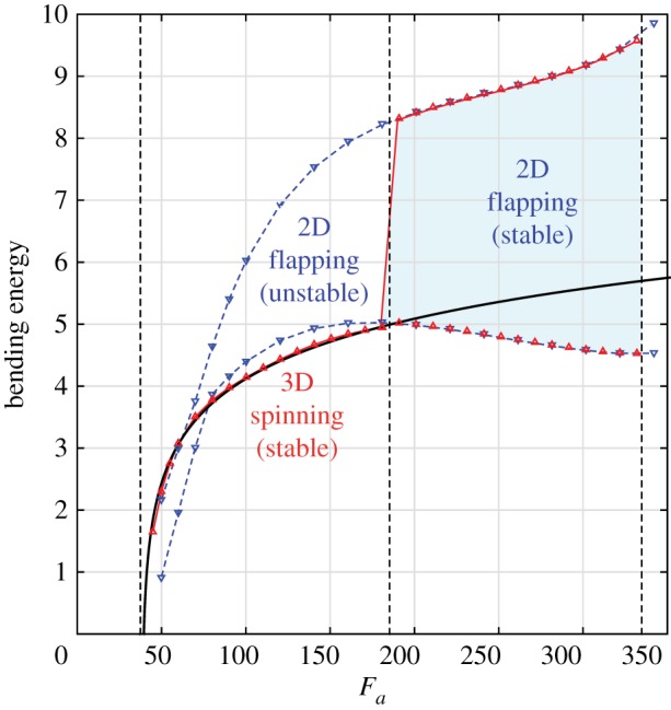
Bending energy versus axial force. The bending energy of spinning motion (red) increases logarithmically with F_a following the curve E_bending = ln(F_a − 38.7) (solid black line). The envelope of the flapping bending energy, from minimum to maximum energy, is depicted for the unstable (confined) 2D flapping for F_a < 188 (blue, down-triangle symbols) and the stable 2D flapping for F_a > 188 (red and blue with symbols). The minimum of the bending energy of flapping starts to decrease near the transition. (Online version in colour.)

To summarize, the results in this section show that the nonlinear dynamics of an elastic filament in a viscous fluid, clamped at one end and subject to a follower compressive force at its free end, is far richer than previously recognized. As the magnitude of the axial force F_a increases, four distinct regimes of dynamical behaviours are observed: (i) a monotonically stable regime, (ii) a regime with decaying oscillations, (iii) 3D spinning motions at a buckled configuration with locked curvature, and (iv) 2D flapping motions where the filament dynamically converges to planar oscillations.

6. Axial force profiles

We examine the robustness of the four regimes identified in §5 to the distribution of axial forces along the filament centreline. Specifically, we consider two force profiles. The first profile consists of a linear force density, with two parameters α and f_a,

$${\mathbf{f}}_{\mathrm{a}}=-f_{\mathrm{a}}[1+\alpha (2s-1)]\mathbf{t}.$$ 6.1

Here, f_a is the intensity of the force density, α ranges from −1 to 1 and αf_a determines the slope of the linear force distribution; negative α corresponds to a force density that decreases as s increases towards the tip of the filament and positive α to a force density that increases towards the filament tip. The total compressive force exerted on the filament is given by $F_{\mathrm{a}}={\int }_0^1{f}_{\mathrm{a}}[1+\alpha (2s-1)]\hspace{0.17em}\text{d}s=f_{\mathrm{a}}$. The second profile consists of a concentrated force f_a at a distance s_a from the base point of the filament

$${\mathbf{f}}_{\mathrm{a}}=-f_{\mathrm{a}}\delta (s-s_{\mathrm{a}})\mathbf{t},$$ 6.2

where δ(s − s_a) is the Dirac delta function and s_a ranges between 0 and 1; s_a = 1 corresponds to the force at the tip of the filament. The total compressive force exerted on the filament is given by $F_{\mathrm{a}}={\int }_0^1{f}_{\mathrm{a}}\delta (s-s_{\mathrm{a}})\hspace{0.17em}\text{d}s=f_{\mathrm{a}}$. A schematic depicting these two profiles is shown in figure 7.

Figure 7.

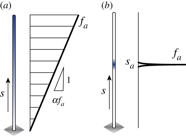
Axial forces. Schematic showing the distribution of the axial forces along the filament centreline: (a) an axial force density that varies linearly from the base of the filament to its tip and (b) the axial force is concentrated at a distance of s_a from the filament base. (Online version in colour.)

In figure 8a, we set F_a = 125 and consider three values of α. For α = −0.5, the axial force decreases towards the filament tip, α = 0 corresponds to a constant force density along the filament, and for α = 1 the axial force increases towards the filament tip. In all three cases, the filament buckles into a locked configuration and undergoes 3D spinning motion. We systematically analyse the behaviour of the filament as a function of the two parameters α and F_a. The results are shown in the parameter space (α, F_a) in figure 8b: black dots correspond to cases where the straight configuration is stable, the solid black line denotes the Hopf bifurcation marking the transition to growing oscillations based on the linear stability analysis of §4. The colourmap denotes the frequency of the nonlinear oscillations of the filament. The filament motion is represented next to each point (α, F_a) by superimposing the filament configuration at various time steps within the oscillation cycle. Force densities that decrease towards the tip of the filament (α < 0) require larger force values F_a to reach the threshold for the Hopf bifurcation. In all cases past the Hopf bifurcation, the filament buckles and undergoes 3D spinning at frequencies larger than the frequencies predicted by the linear stability analysis.

Figure 8.

Gallery of filament oscillations. In (a,b), filaments subject to linear distribution of axial forces exhibit buckling and 3D spinning motion only despite changes in parameter α. But the threshold of instability decreases and the radius of the circle formed by the filament tips increases for higher α. In (c,d), filaments are subjected to a concentrated axial force at varying location s_a, leading to qualitatively distinct regimes of motion. For s_a < 0.5, the distal tip of the filament remains taller than the largest circle formed by the spinning motion. When forces are concentrated closer to the tip, we observe the 3D spinning to 2D flapping transition of figure 4. Note that, in both (b,d), changes in the threshold of initial instability of static straight equilibrium are well matched by the linear stability analysis (solid black lines). F_a = 125 and 300, respectively, for snapshots shown in (a,c). (Online version in colour.)

In figure 8c, we consider a concentrated force F_a = 300 and vary its location along the filament. At s_a = 0.3, the filament buckles into a locked curvature and spins about the z-direction. The filament exhibits large curvatures near the point of application of the axial force, with flatter curvature near the tip. For s_a = 0.5, the filament also buckles, exhibiting similar behaviour but more gradual variations in curvature. For s_a = 0.9, the filament undergoes planar flapping motion, even when subject to non-planar perturbations. A gallery of the filament behaviour as a function of the two parameters s_a and F_a is depicted in figure 8d. The filament first transitions from a straight configuration to 3D spinning motion. A second transition occurs from 3D spinning to a 2D flapping motion as s_a and F_a increase further, as highlighted by the dashed black line in the upper right corner of the parameter space. In dimensional form, the force threshold F_aB/L² required to trigger these instabilities increases as the filament length decreases.

For both profiles of axial forces, the first transition, marking the destabilization of the straight configuration under the distribution of axial forces F_a, is captured by the linear stability analysis of §4. As we vary the two parameters corresponding to each forcing profile, (α, F_a) and (s_a, F_a), respectively, linear stability analysis indicates a transition from a stable to an unstable straight configuration through a Hopf bifurcation as shown in figure 9. However, linear stability analysis predicts growing planar oscillations at frequencies less than the frequencies of the 3D spinning motions obtained in the nonlinear system. Further, this linear analysis does not capture the second transition, from non-planar spinning to planar flapping, observed in the concentrated force profile.

Figure 9.

Linear stability analysis. We plot the full results of linear stability analysis for (a) the linear forcing profiles and (b) the concentrated forcing profiles. The real parts of λ indicate the stability of straight equilibrium, while the imaginary parts predict the frequency of oscillations. Similar to figure 5, the imaginary parts become positive before the real parts, indicating the existence of decaying oscillations. The frequencies predicted here by linear stability are in rough agreement with those shown in figure 8.

Based on the gallery of filament oscillations reported in figure 8, the following observations are in order. (1) The first buckling instability, captured by the linear stability analysis, always leads to 3D spinning motions. (2) The second transition from 3D spinning to 2D flapping seems to occur when the force distribution is biased towards the tip of the filament; as explored in more detail next. (3) Away from the transition thresholds, the filament behaviour is insensitive to changes in the parameters of the axial force, even to changes in the form of the axial force profile. These observations could have important implications for the relevance of this instability-driven mechanism to biological cilia and flagella as discussed in §8.

To better understand the effect of the distribution of axial forces along the filament on this transition from 3D spinning to 2D flapping, we introduce a forcing profile that allows us to continuously change from a linearly distributed force profile to a force concentrated at the filament tip. To this end, we consider

$${\mathbf{f}}_{\mathrm{a}}=-f_{\mathrm{a}}(p+1)s^p\hspace{0.17em}\mathbf{t},$$ 6.3

where p controls how much force is concentrated near the tip in a gradual way. At p = 1, the force expression in (6.3) is identical to that in (6.1) for α = 1. As p → ∞, this force converges to (6.2) for s_a = 1. Again, we have $F_{\mathrm{a}}={\int }_0^1{f}_{\mathrm{a}}(p+1)s^p\hspace{0.17em}\text{d}s=f_{\mathrm{a}}$.

Figure 10 is a phase diagram that summarizes the behaviour of the filament as a function of p and F_a. We find that for a big range of axial forces, potentially exceeding the biologically relevant range, when p = 1, that is, for a linear force distribution, there is no transition from 3D spinning to 2D flapping motions. As p exceeds 1, that is, for force distributions that are larger towards the filament tip, we observe a transition from spinning to flapping motions at biologically relevant values of the axial force F_a (as discussed in §8). For even larger forces, another transition occurs from planar flapping to toroidal flapping motions, and even to chaotic-like behaviour. Representative trajectories of the mean position of the filament are superimposed onto the phase space to illustrate the complex nature of these motions. These results indicate that higher concentrations of axial forces near the distal portion of the microfilament accelerate the development of complex behaviours.

Figure 10.

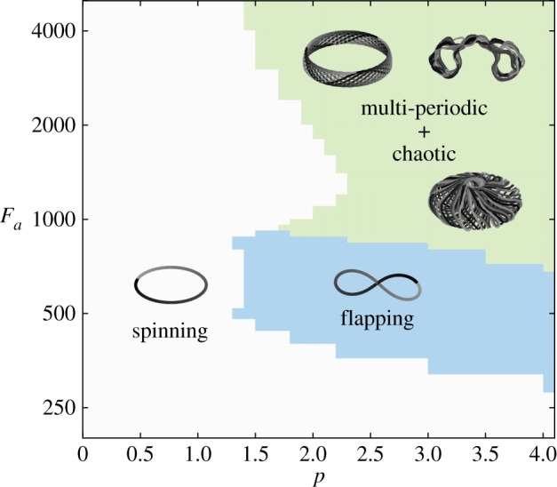
Phase diagram based on power-law forcing profiles. We expand the findings of figure 8 by showing the transition behaviours at much higher F_a using the power-law forcing profiles of (6.3). We see that only when the axial forces increase at a power larger than ≈ 1.5 would 3D spinning transition to 2D flapping. Moreover, at very large forces, we can also obtain much more exotic trajectories. The patterns shown above are formed by the average positions of the filament over its arc-length (grey scale represents passage of time). (Online version in colour.)

It is worth noting here that we calculated the Lyapunov exponents for large values of F_a concentrated at the tip of the filament leading to chaotic-like behaviour. Namely, we calculated the Lyapunov exponents for arbitrary initial conditions based on finite separation in the mean position of the filament (results not shown). Upon removal of a rotational symmetry due to the initial Euler buckling, trajectories from two nearby initial conditions diverge initially, but saturate at a large distance, giving rise to Lyapunov exponents that are consistent with chaos. Similar chaotic trajectories are reported in recent models of active biological filaments [46]. It is not clear if this chaotic behaviour is biologically relevant for a beating flagellum because these large F_a may lie beyond the capabilities of the dynein molecular motors. However, it is not completely surprising to obtain chaotic behaviour in this dissipative system owing to the resemblance of the filament equations of motion to the Kuramoto–Sivashinsky equation that models diffusive instabilities in a laminar flame front.

To conclude this section, we note that the spinning to flapping transition is insensitive to the anisotropy in the fluid drag force. Our numerical experiments show that, when changing γ, the filament continues to transition from 3D spinning to planar flapping then to 3D motion, albeit requiring a different amount of axial force. This observation will allow us to ignore drag anisotropy in our reduced-order, bead–spring model discussed next.

7. Bead–spring model

The elastic filament, subject to an axial force at the free tip, buckles and undergoes 3D rigid spinning at a locked curvature before it transitions to 2D flapping motions at large values of F_a. These nonlinear effects are not captured by the linear stability analysis. Here, we consider a bead–spring model of the filament with the aim of reproducing these nonlinear effects with the minimum number of degrees of freedom.

We model the elastic filament as a chain of N beads is located at r_i, where i = 1, …, N, and connected successively via inextensible rods of length L/N from the origin ${\mathbf{r}}_o={(0,0,0)}^{\mathsf{T}}$ (see figure 11 for a two-link example). To emulate the filament elasticity, we attach to each bead i ≠ N a torsional spring that produces a spring moment M_s,i = −Kψ_i, where K is the spring constant and ${\psi }_i:={\cos }^{-1}({\mathbf{t}}_{i-1}\cdot {\mathbf{t}}_i)$ is the angle between successive links, with t _i: = (r_i − r_i−1)/‖r_i − r_i−1‖. We enforce the clamped boundary condition at r_o weakly by including a spring moment $M_{s,o}=-K{\cos }^{-1}(e_3\cdot {\mathbf{t}}_1)$, proportional to the angle between the equilibrium axis and the first link. The chain is subject to an axial force acting at its tip, on bead N, of the form F_a = −F_at _N. Each bead is subject to an isotropic drag force F _h,i = −ζv_i.

Figure 11.

Two-link chain. (a) A two-link chain subject to an axial follower force F_a = 4, concentrated at its tip. (b) Starting from a straight configuration, non-planar perturbations lead to 3D spinning motions. (c) By symmetry, planar perturbations lead to flapping motions, but these solutions are unstable to the three-dimensional perturbations. (d) The maximum bending energy of planar flapping is larger than the constant bending energy of the spinning motion. (Online version in colour.)

We rewrite these quantities in non-dimensional form using the total chain length L as the characteristic length scale and L³ζ/K as the characteristic time scale. To this end, the non-dimensional force is given by F_aL/K as opposed to the non-dimensional force in the filament model F_aL²/B. Thus, the range of relevant values of the dimensionless force in the chain model may differ from that of the filament model. In the following, we consider all quantities to be non-dimensional.

We write the position vector to bead i as r_i = r_i−1 + t_i/N, where the vector t _i is expressed in terms of the spherical coordinates θ_i and ϕ_i attached to bead i; namely, ${\mathbf{t}}_i\equiv {(\cos {\theta }_i\cos {\varphi }_i,\cos {\theta }_i\sin {\varphi }_i,\sin {\theta }_i)}^{\mathsf{T}}$. We can then explicitly express the variations δr_i and use the principle of virtual work,

$${\mathbf{F}}_a\cdot \delta {\mathbf{r}}_N+\sum _{i=1}^N{\mathbf{F}}_{h,i}\cdot \delta {\mathbf{r}}_i+\sum _{i=0}^{N-1}{M}_{s,i}\delta {\psi }_i=0,$$ 7.1

to obtain 2N governing equations for an N-link chain in terms of θ_i and ϕ_i. Note that, after proper non-dimensionalization, the planar two-link equations of [29] can be recovered by setting ϕ_i = 0, i = 0, 1. For N = 1, inextensibility dictates that the tip follower force has no effect, thus the straight equilibrium configuration is globally asymptotically stable. The system admits both spinning and flapping trajectories for all N ≥ 2. However, since torsion is related to ∂³r/∂s³, to account for the effects of torsion, we need N ≥ 3.

In figure 11, we show the behaviour of a two-link model subject to an axial follower force F_a = 4, concentrated at its tip. Starting from a straight configuration, non-planar perturbations bring the chain into 3D spinning motion. Planar flapping motions can only be obtained for planar initial perturbations, and are unstable to non-planar perturbations, consistent with the full filament model. The bending energy of spinning is constant over time while the bending energy of the flapping motion oscillates as a function of time, accessing larger energy values than the spinning motion, similar to the full filament model.

We linearize the equations of motion for two- and three-link chains and examine the dominant eigenvalues of the linear system. The state variables θ_i from ϕ_i decouple at the linear level, similar to the decoupling of curvature and torsion in the full filament model. Figure 12 shows the nonlinear frequencies of the two- and three-link chains, subject to 3D and 2D perturbations, and compares them with the results of the linear stability analysis. As in the full filament model, a Hopf bifurcation leads to sustained oscillations of the chains, and, as in figure 5, the frequencies of 3D spinning are consistently larger than the frequencies of planar flapping of the confined chain. The latter solutions are unstable to non-planar perturbations.

Figure 12.

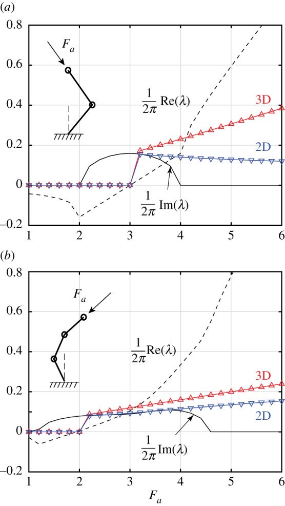
Linear stability of two-link and three-link chains. Nonlinear frequencies of the (a) two- and (b) three-link chains compared with the dominant eigenvalue from linear stability analysis. Similar to figure 5, the frequency of 3D spinning is consistently larger than the frequency of planar flapping. The latter is unstable to non-planar perturbations. (Online version in colour.)

In order to examine the transition from 3D spinning to 2D flapping motions in the chain model, we perform a continuation-type analysis for five different link numbers N = 2–6 (see electronic supplementary material, movie S5). We stop at N = 6 because it corresponds to the chain with the smallest number of links that unambiguously exhibit the transition from 3D spinning to 2D flapping. For each N, we start with F_a = 0 and increase its value systematically as follows: we let the chain settle into a stable solution at a given value of F_a, we then increase the value of F_a to obtain a new stable solution, and repeat successively. In figure 13a, we show the maximum and minimum envelope of the bending energy as a function of F_a. Since the 3D spinning motions correspond to rigid rotations at a locked curvature of the buckled filament, the bending energy is constant, and its maximum and minimum are equal. Observe that spinning becomes unstable at large values of F_a only for N ≥ 3. In figure 13b, we illustrate the chain behaviour by superimposing several snapshots of the same chain during one period of its oscillations. We show the filament behaviour as a function of the number of links N and the tip force F_a. For 3 ≤ N < 6, we observe a transition from spinning to ‘windmilling’ motions, where the chain or part of the chain rotates (windmills) roughly about an axis in the (x, y)-plane. For N = 6, planar flapping solutions become stable for a range of F_a. This is also true for N > 6 (results not shown for brevity). In the limit of large N, the discrete chain model exhibits similar results to the discrete filament model of §3, albeit without drag anisotropy. That is to say, instability-driven oscillations occur under the assumption of local isotropic drag, indicating that they are insensitive to the hydrodynamic force model. This is in contrast to systems that require hydrodynamic interactions along the chain to trigger sustained oscillations [47].

Figure 13.

Transition to non-spinning solutions of the bead–spring models. We perform a continuation-type analysis for different numbers of links, where we let the chain settle onto a stable solution at a given F_a and successively increase F_a to obtain new stable solutions. (a) The maximum and minimum envelope of the resultant bending energy as a function of F_a. Spinning motions become unstable at large F_a for N ≥ 3. (b) Chain behaviour as a function of the number of links and F_a flapping solutions become stable for a fixed range of F_a only at N = 6. (Online version in colour.)

The transition away from the 3D spinning motion is consistent with our physical intuition in §5. When spinning, the work done by the tip force is balanced by the constant elastic energy stored in the locked configuration of the chain and the work dissipated through viscous drag due to the ‘rigid’ rotation about the z-axis. As the tip force F_a increases, to maintain this balance, the three-link chain opts to minimize time-dependent deformations by rigidly rotating the whole chain about an axis in the (x, y)-plane. This rotation is permitted because the clamped boundary condition in the chain model is imposed weakly, via an elastic spring at O. Since these rotations activate the elastic spring at the base, the corresponding elastic energy is non-zero. Also, these rotations lead to larger linear velocities and thus larger drag forces (that is, larger dissipation) than rotations about the z-axis. For four- and five-link chains, the upper link of the chain succumbs first under the axial force and begins to rotate in a windmill-like motion, as illustrated in figure 13b. However, as the number of links increase, these hybrid solutions—consisting of rigid spinning about the z-axis with windmill-like rotations that are spatially localized at the distal links—become unstable. At N = 6, the chain clearly exhibits wave-like deformations.

8. Discussion

We considered an elastic microfilament, clamped at one end in a viscous fluid, subject to a distribution of axial forces. We identified two major transitions in the filament behaviour. First, the filament transitions from a straight configuration to a buckled configuration, with locked curvature, and undergoes 3D spinning. The second transition occurs at larger values of the axial force and marks a destabilization of the 3D spinning motions, giving rise to 2D flapping oscillations. These periodic motions, both 3D spinning and 2D flapping, are robust to large perturbations in the filament configuration. They are also robust, away from the bifurcation values, to perturbations in the parameters of the axial forces, and even to changes in the force profile altogether (as long as the force density increases sufficiently nonlinearly towards the tip of the filament). These findings, although in the context of a simplified model, support the idea that an open-loop, instability-driven mechanism could explain not only the origin of sustained oscillations but also the wide variety of periodic beating patterns observed in cilia and flagella.

Cilia and flagella, despite their highly conserved internal axoneme structure across cell types, exhibit distinct beating patterns depending on the cell type, environment and function. For example, sperm cells propel themselves by planar wave-like deformations of their flagellum [48]. The biflagellate algal cell Chlamydomonas swim using synchronized flapping oscillations of their flagella, referred to as ‘breast stroke’, and can transition to unsynchronized wave-like oscillations, referred to as ‘free style’, that allow them to turn and reorient themselves [49,50]. In a densely packed ciliated surface, motile cilia often beat in 3D patterns, with an asymmetry in their effective and recovery stroke. A gallery of various planar and non-planar cilia beating patterns can be found in [6,7].

The model presented in this paper does not accurately represent the intricate internal structure of cilia. It rather assumes that its net effect on the cilium centreline can be approximated by a distribution of axial forces of constant magnitude. An accurate representation of the effect of the axoneme structure on the centreline motion would give rise to a distribution of axial and normal forces that are coupled to the centreline geometry. These limitations notwithstanding, we use the current model to roughly gauge whether the instability-driven oscillations and the transitions reported in this study are relevant to the mechanics of cilia and flagella. To this end, we provide a rough estimate of the total axial force that is biologically attainable. We estimate the total amount of forces that the dynein motors provide inside a typical cilium. The axoneme consists typically of ‘9 + 2’ microtubule doublets, with nine outer doublets and a central pair (figure 1). Dynein molecules form an array of cross-bridges between pairs of outer microtubule doublets. The force exerted on microtubules by a single molecular motor is known to be of the order of a few pico-newtons. So assuming eight dynein arms per 100 nm and 3–8 pN of force per dynein arm [51], we would get a per-doublet force density estimate of 200–$600\hspace{0.17em}\hspace{0.17em}\text{pN}\cdot \mu {\text{m}}^{-1}$. This gives us about 2–$5\hspace{0.17em}\text{nN}\cdot \mu {\text{m}}^{-1}$ per cilium assuming all nine doublets are activated. In reality, because of the internal structural damping and other reaction forces (most doublets experience dynein forces in both compressive and extensile directions), the total compressive force density is likely to be much smaller. In our model, a force density of the order of $20\hspace{0.17em}\hspace{0.17em}\text{pN}\cdot \mu {\text{m}}^{-1}$ can lead to sustained oscillations and is sufficient to even induce the transition from 3D spinning to a planar flapping regime. This calculation is based on the cilia length and bending rigidity estimate of table 1, where we have chosen a typical length of 20 µm as cilia and flagella can vary in length between 10 and 50 µm, and a high stiffness value of $800\hspace{0.17em}\hspace{0.17em}\text{pN}\cdot \mu {\text{m}}^2$ compared to values of 25–$800\hspace{0.17em}\hspace{0.17em}\text{pN}\cdot \mu {\text{m}}^2$ reported in the literature [30,42,52–54]. These numbers suggest that the axial forces due to dynein activity in cilia and flagella should be large enough to support these instability-driven oscillations, as noted in more elaborate models of [4,5,28].

Another important consideration for exploring the relevance of these instability-driven oscillations to biological cilia is that cilia often exhibit asymmetric beating patterns. To account for asymmetric oscillations in our filament model, we incorporate a non-zero reference curvature of the filament. Experimental evidence from the algal cells Chlamydomonas supports the notion that their flagella are naturally curved [3]. In our model, we set M = B(κ − κ_o), where κ_o is a non-zero reference curvature. We consider κ_o = 2πd₁, as depicted schematically in the top of figure 14a. Figure 14 shows the filament dynamics under three values of the axial force F_a at the free tip of the filament. We identify three distinct behaviours of the naturally curved filament: (i) ‘asymmetric’ spinning (figure 14b), reminiscent of the spinning behaviour of the naturally straight filament, but here the spinning axis is not normal to the base wall to which the filament is clamped; (ii) ‘asymmetric’ precession while flapping (figure 14c), where the flapping motion is combined with a slow precession about the vertical axis, and flapping frequency is about five times faster than the precession frequency; and (iii) ‘asymmetric’ flapping (figure 14d) that is nearly, but not completely, planar; the filament switches between the left and right sides of a flapping plane in an alternating fashion, as evident from the shadows in the inset of figure 14d. These regimes can be cleanly delineated from the time evolution of a cumulative rotation angle θ, defined in the (x, y)-plane as the angle to the vertical projection of the filament tip; see the bottom schematic in figure 14a. In the top row of figure 14b–d, we plot the change in θ after the filament reaches its limit cycle behaviour. At F_a = 100 (figure 14b), θ changes to be monotonic in time, indicating that the filament is simply spinning. At F_a = 200 (figure 14c), the fast periodic fluctuation of θ reflects the flapping motion, and the slow drift of its average value captures the filament precession. At F_a = 250 (figure 14c), θ varies in (−π, π], indicating that the motion is purely flapping. Owing to the asymmetry incorporated in the system, the vertical position z for the filament tip changes with time in all three behaviours; see bottom row of figure 14b–d. In particular, over one period of oscillation (some highlighted in grey in figure 14), the filament tip periodically gets closer to and then further away from the base wall, in a way reminiscent of the effective and recovery strokes in ciliary beating patterns.

Figure 14.

Asymmetric beating patterns. (a) A naturally curved filament with a reference curvature of κ_o = 2πd₁ is subjected to an axial force F_a at its tip. We define the rotation angle θ in the (x, y)-plane associated with the vertical projection of the tip point. (b) At F_a = 100, an asymmetric 3D spinning pattern develops: θ monotonically decreases and the vertical tip position z varies periodically. (c) At F_a = 200, the filament engages in asymmetric flapping while it slowly precesses about the vertical axis: θ drifts on average. (d) At F_a = 250, the asymmetric flapping is nearly planar but switches between flapping on the left and right sides of that plane: θ is periodic. The filament snapshots are taken from the regions highlighted in grey. (Online version in colour.)

The work in this study is a first step towards understanding the interplay between the molecular motor activity, the elastic properties of biological filaments, and the fluid mechanical forces in generating the wide variety of beating patterns observed across flagellated cells and in the transitions between multiple beating modes in the same cell as the level of molecular motor activity changes. This work focused on the case of a single filament in a viscous fluid, using the resistive force theory. One of the main advantages of this simple model is that it avoids the requirement of numerous material parameters, unknown experimentally, such as those needed in a full-fledged finite-element simulation involving more details of the internal structure of flagella [5,55]. This simple model also allows us to focus on the fundamental mechanisms underlying flagellar oscillations and the various transitions that could potentially be responsible for the variety of beating patterns observed in nature. However, a few remarks on the limitations of the model are in order. Our model does not fully reflect the internal mechanics of cilia. In ongoing work, we are deriving the equations of motion and effective forces acting on the centreline from more elaborate, coupled, multi-filament models of the axoneme structure. The present model does not account for the long-range hydrodynamic effects of viscous fluids. Future extensions of this work will account for the full hydrodynamics, using a combination of slender body theory and regularized Stokeslet formulation, in the presence of the cell body or the cell wall [54,56]. Future work will also focus on the effects of anisotropy in the bending rigidity matrix B, which encodes information about the internal axoneme structure. Experimental evidence indicates that the presence or the absence of certain structures within the flagellum could lead to 3D versus planar beating patterns in the Chlamydomonas flagella [11]. This suggests that anisotropy of bending rigidity could be another crucial effect responsible for the varied motion of cilia and flagella. It is also important to account for the effects of the intrinsic oscillations of the dynein motor forces due to the time scales of their binding and unbinding to microtubules and due to thermal fluctuations [51]. Lastly, this instability-driven mechanism could have implications for the coordinations of multiple active filaments with non-local hydrodynamic interactions [54]. The presence of neighbouring filaments and other solid boundaries may affect the transition thresholds and bias planar versus non-planar beating patterns.

Data accessibility

Additional details are available in the electronic supplementary material.

Authors' contributions

E.K. designed the research. F.L., H.G. and E.K. performed the research, analysed the results and wrote the paper.

Competing interests

We declare we have no competing interests.

Funding

This work is supported in part by NSF INSPIRE grant 160844, ARO grant no. W911NF-16-1-0074 and ONR grant no. N00014-17-1-2062.

References

- 1.Brokaw CJ. 1971. Bend propagation by a sliding filament model for flagella. J. Exp. Biol. 55, 289–304. [DOI] [PubMed] [Google Scholar]
- 2.Lindemann CB. 1994. A ‘geometric clutch’ hypothesis to explain oscillations of the axoneme of cilia and flagella. J. Theor. Biol. 168, 175–189. ( 10.1006/jtbi.1994.1097) [DOI] [Google Scholar]
- 3.Sartori P, Geyer VF, Scholich A, Jülicher F, Howard J. 2016. Dynamic curvature regulation accounts for the symmetric and asymmetric beats of Chlamydomonas flagella. Elife 5, e13258 ( 10.7554/eLife.13258) [DOI] [PMC free article] [PubMed] [Google Scholar]
- 4.Bayly P, Dutcher S. 2016. Steady dynein forces induce flutter instability and propagating waves in mathematical models of flagella. J. R. Soc. Interface 13, 20160523 ( 10.1098/rsif.2016.0523) [DOI] [PMC free article] [PubMed] [Google Scholar]
- 5.Hu T, Bayly PV. 2018. Finite element models of flagella with sliding radial spokes and interdoublet links exhibit propagating waves under steady dynein loading. Cytoskeleton 75, 185–200. ( 10.1002/cm.v75.5) [DOI] [PubMed] [Google Scholar]
- 6.Sleigh MA. 1968. Patterns of ciliary beating. Symp. Soc. Exp. Biol. 22, 131–150. [PubMed] [Google Scholar]
- 7.Brennen C, Winet H. 1977. Fluid mechanics of propulsion by cilia and flagella. Annu. Rev. Fluid Mech. 9, 339–398. ( 10.1146/annurev.fl.09.010177.002011) [DOI] [Google Scholar]
- 8.Blake JR. 1972. A model for the micro-structure in ciliated organisms. J. Fluid Mech. 55, 1–23. ( 10.1017/S0022112072001612) [DOI] [Google Scholar]
- 9.Chwang A, Wu TY. 1971. A note on the helical movement of micro-organisms. Proc. R. Soc. Lond. B 178, 327–346. ( 10.1098/rspb.1971.0068) [DOI] [PubMed] [Google Scholar]
- 10.Hirokawa N, Tanaka Y, Okada Y, Takeda S. 2006. Nodal flow and the generation of left-right asymmetry. Cell 125, 33–45. ( 10.1016/j.cell.2006.03.002) [DOI] [PubMed] [Google Scholar]
- 11.Meng D, Cao M, Oda T, Pan J. 2014. The conserved ciliary protein Bug22 controls planar beating of Chlamydomonas flagella. J. Cell Sci. 127, 281–287. ( 10.1242/jcs.140723) [DOI] [PubMed] [Google Scholar]
- 12.Brokaw CJ. 2009. Thinking about flagellar oscillation. Cell Motil. Cytoskeleton 66, 425–436. ( 10.1002/cm.v66:8) [DOI] [PubMed] [Google Scholar]
- 13.Riedel-Kruse IH, Müller C, Oates AC. 2007. Synchrony dynamics during initiation, failure, and rescue of the segmentation clock. Science 317, 1911–1915. ( 10.1126/science.1142538) [DOI] [PubMed] [Google Scholar]
- 14.Brokaw CJ. 1972. Computer simulation of flagellar movement: I. Demonstration of stable bend propagation and bend initiation by the sliding filament model. Biophys. J. 12, 564–586. ( 10.1016/S0006-3495(72)86104-6) [DOI] [PMC free article] [PubMed] [Google Scholar]
- 15.Brokaw CJ, Rintala DR. 1975. Computer simulation of flagellar movement. III. Models incorporating cross-bridge kinetics. J. Mechanochem. Cell Motility 3, 77–86. [PubMed] [Google Scholar]
- 16.Brokaw CJ. 1985. Computer simulation of flagellar movement. VI. Simple curvature-controlled models are incompletely specified. Biophys. J. 48, 633–642. ( 10.1016/S0006-3495(85)83819-4) [DOI] [PMC free article] [PubMed] [Google Scholar]
- 17.Hines M, Blum JJ. 1983. Three-dimensional mechanics of eukaryotic flagella. Biophys. J. 41, 67–79. ( 10.1016/S0006-3495(83)84406-3) [DOI] [PMC free article] [PubMed] [Google Scholar]
- 18.Murase M, Hines M, Blum JJ. 1989. Properties of an excitable dynein model for bend propagation in cilia and flagella. J. Theor. Biol. 139, 413–430. ( 10.1016/S0022-5193(89)80219-X) [DOI] [PubMed] [Google Scholar]
- 19.Hilfinger A, Riedel-Kruse I, Howard J, Jülicher F. 2009. How molecular motors shape the flagellar beat. Biophys. J. 96, 196a ( 10.1016/j.bpj.2008.12.1051) [DOI] [PMC free article] [PubMed] [Google Scholar]
- 20.Hilfinger A, Chattopadhyay AK, Jülicher F. 2009. Nonlinear dynamics of cilia and flagella. Phys. Rev. E 79, 051918 ( 10.1103/PhysRevE.79.051918) [DOI] [PubMed] [Google Scholar]
- 21.Camalet S, Jülicher F. 2000. Generic aspects of axonemal beating. New J. Phys. 2, 24 ( 10.1088/1367-2630/2/1/324) [DOI] [Google Scholar]
- 22.Lindemann CB. 1994. A model of flagellar and ciliary functioning which uses the forces transverse to the axoneme as the regulator of dynein activation. Cell Motil. Cytoskeleton 29, 141–154. ( 10.1002/(ISSN)1097-0169) [DOI] [PubMed] [Google Scholar]
- 23.Lindemann CB. 2002. Geometric clutch model version 3: the role of the inner and outer arm dyneins in the ciliary beat. Cell Motil. Cytoskeleton 52, 242–254. ( 10.1002/(ISSN)1097-0169) [DOI] [PubMed] [Google Scholar]
- 24.Bayly PV, Wilson KS. 2014. Equations of interdoublet separation during flagella motion reveal mechanisms of wave propagation and instability. Biophys. J. 107, 1756–1772. ( 10.1016/j.bpj.2014.07.064) [DOI] [PMC free article] [PubMed] [Google Scholar]
- 25.Dowell EH, Curtiss HC, Scanlan RH, Sisto F. 1989. A modern course in aeroelasticity, vol. 3 Berlin, Germany: Springer. [Google Scholar]
- 26.Paidoussis MP. 1998. Fluid-structure interactions: slender structures and axial flow, vol. 1 New York, NY: Academic Press. [Google Scholar]
- 27.Paidoussis MP. 2008. The canonical problem of the fluid-conveying pipe and radiation of the knowledge gained to other dynamics problems across applied mechanics. J. Sound Vib. 310, 462–492. ( 10.1016/j.jsv.2007.03.065) [DOI] [Google Scholar]
- 28.Han J, Peskin CS. 2018. Spontaneous oscillation and fluid–structure interaction of cilia. Proc. Natl Acad. Sci. USA 115, 4417–4422. ( 10.1073/pnas.1712042115) [DOI] [PMC free article] [PubMed] [Google Scholar]
- 29.De Canio G, Lauga E, Goldstein RE. 2017. Spontaneous oscillations of elastic filaments induced by molecular motors. J. R. Soc. Interface 14, 20170491 ( 10.1098/rsif.2017.0491) [DOI] [PMC free article] [PubMed] [Google Scholar]
- 30.Eloy C, Lauga E. 2012. Kinematics of the most efficient cilium. Phys. Rev. Lett. 109, 038101 ( 10.1103/PhysRevLett.109.038101) [DOI] [PubMed] [Google Scholar]
- 31.Sartori P, Geyer VF, Howard J, Jülicher F. 2016. Curvature regulation of the ciliary beat through axonemal twist. Phys. Rev. E 94, 042426 ( 10.1103/PhysRevE.94.042426) [DOI] [PubMed] [Google Scholar]
- 32.Lindemann CB, Macauley LJ, Lesich KA. 2005. The counterbend phenomenon in dynein-disabled rat sperm flagella and what it reveals about the interdoublet elasticity. Biophys. J. 89, 1165–1174. ( 10.1529/biophysj.105.060681) [DOI] [PMC free article] [PubMed] [Google Scholar]
- 33.Pelle DW, Brokaw CJ, Lesich KA, Lindemann CB. 2009. Mechanical properties of the passive sea urchin sperm flagellum. Cell Motil. Cytoskeleton 66, 721–735. ( 10.1002/cm.v66:9) [DOI] [PubMed] [Google Scholar]
- 34.Gadêlha H, Gaffney EA, Goriely A. 2013. The counterbend phenomenon in flagellar axonemes and cross-linked filament bundles. Proc. Natl Acad. Sci. USA 110, 12 180–12 185. ( 10.1073/pnas.1302113110) [DOI] [PMC free article] [PubMed] [Google Scholar]
- 35.Coy R, Gadêlha H. 2017. The counterbend dynamics of cross-linked filament bundles and flagella. J. R. Soc. Interface 14, 20170065 ( 10.1098/rsif.2017.0065) [DOI] [PMC free article] [PubMed] [Google Scholar]
- 36.Bergou M, Wardetzky M, Robinson S, Audoly B, Grinspun E. 2008. Discrete elastic rods. ACM Trans. Graphics 27, 63 ( 10.1145/1360612.1360662) [DOI] [Google Scholar]
- 37.Gazzola M, Dudte L, McCormick A, Mahadevan L. 2018. Forward and inverse problems in the mechanics of soft filaments. R. Soc. open sci. 5, 171628 ( 10.1098/rsos.171628) [DOI] [PMC free article] [PubMed] [Google Scholar]
- 38.Monteith CE, Brunner ME, Djagaeva I, Bielecki AM, Deutsch JM, Saxton WM. 2016. A mechanism for cytoplasmic streaming: kinesin-driven alignment of microtubules and fast fluid flows. Biophys. J. 110, 2053–2065. ( 10.1016/j.bpj.2016.03.036) [DOI] [PMC free article] [PubMed] [Google Scholar]
- 39.Audoly B, Pomeau Y. 2010. Elasticity and geometry: from hair curls to the non-linear response of shells. Oxford, UK: Oxford University Press. [Google Scholar]
- 40.Kirchhoff G. 1859. Ueber das Gleichgewicht und die Bewegung eines unendlich dünnen elastischen Stabes. J. Reine Angew. Math. 56, 285–313. ( 10.1515/crll.1859.56.285) [DOI] [Google Scholar]
- 41.Lauga E, Powers TR. 2009. The hydrodynamics of swimming microorganisms. Rep. Prog. Phys. 72, 096601 ( 10.1088/0034-4885/72/9/096601) [DOI] [Google Scholar]
- 42.Xu G, Wilson KS, Okamoto RJ, Shao JY, Dutcher SK, Bayly PV. 2016. Flexural rigidity and shear stiffness of flagella estimated from induced bends and counterbends. Biophys. J. 110, 2759–2768. ( 10.1016/j.bpj.2016.05.017) [DOI] [PMC free article] [PubMed] [Google Scholar]
- 43.Ritz W. 1909. Uber eine neue Methode zur Losung gewisser Variationsprobleme der mathematischen Physik. J. Math. 1909, 1–61. ( 10.1515/crll.1909.135.1) [DOI] [Google Scholar]
- 44.MacDonald J. 1933. Successive approximations by the Rayleigh-Ritz variation method. Phys. Rev. 43, 830 ( 10.1103/PhysRev.43.830) [DOI] [Google Scholar]
- 45.Bayly P, Wilson K. 2015. Analysis of unstable modes distinguishes mathematical models of flagellar motion. J. R. Soc. Interface 12, 20150124 ( 10.1098/rsif.2015.0124) [DOI] [PMC free article] [PubMed] [Google Scholar]
- 46.Pearce SP, Heil M, Jensen OE, Jones GW, Prokop A. 2018. Curvature-sensitive kinesin binding can explain microtubule ring formation and reveals chaotic dynamics in a mathematical model. Bull. Math. Biol. 80, 3002–3022. ( 10.1007/s11538-018-0505-4) [DOI] [PubMed] [Google Scholar]
- 47.Laskar A, Singh R, Ghose S, Jayaraman G, Kumar PS, Adhikari R. 2013. Hydrodynamic instabilities provide a generic route to spontaneous biomimetic oscillations in chemomechanically active filaments. Sci. Rep. 3, 1964 ( 10.1038/srep01964) [DOI] [PMC free article] [PubMed] [Google Scholar]
- 48.Woolley DM, Crockett RF, Groom WD, Revell SG. 2009. A study of synchronisation between the flagella of bull spermatozoa, with related observations. J. Exp. Biol. 212, 2215–2223. ( 10.1242/jeb.028266) [DOI] [PubMed] [Google Scholar]
- 49.Leptos KC, Wan KY, Polin M, Tuval I, Pesci AI, Goldstein RE. 2013. Antiphase synchronization in a flagellar-dominance mutant of Chlamydomonas. Phys. Rev. Lett. 111, 158101 ( 10.1103/PhysRevLett.111.158101) [DOI] [PMC free article] [PubMed] [Google Scholar]
- 50.Wan KY, Leptos KC, Goldstein RE. 2014. Lag, lock, sync, slip: the many ‘phases’ of coupled flagella. J. R. Soc. Interface 11, 20131160 ( 10.1098/rsif.2013.1160) [DOI] [PMC free article] [PubMed] [Google Scholar]
- 51.Shingyoji C, Higuchi H, Yoshimura M, Katayama E, Yanagida T. 1998. Dynein arms are oscillating force generators. Nature 393, 711–714. ( 10.1038/31520) [DOI] [PubMed] [Google Scholar]
- 52.Guo H, Nawroth JC, Ding Y, Kanso E. 2014. Cilia beating patterns are not hydrodynamically optimal. Phys. Fluids 26, 091901 ( 10.1063/1.4894855) [DOI] [Google Scholar]
- 53.Guo H, Kanso E. 2016. Evaluating efficiency and robustness in cilia design. Phys. Rev. E 93, 033119 ( 10.1103/PhysRevE.93.033119) [DOI] [PubMed] [Google Scholar]
- 54.Guo H, Fauci L, Shelley MJ, Kanso E. 2018. Bistability in the synchronization of actuated microfilaments. J. Fluid Mech. 836, 304–323. ( 10.1017/jfm.2017.816) [DOI] [Google Scholar]
- 55.Chen D, Zhong Y. 2015. A computational model of dynein activation patterns that can explain nodal cilia rotation. Biophys. J. 109, 35–48. ( 10.1016/j.bpj.2015.05.027) [DOI] [PMC free article] [PubMed] [Google Scholar]
- 56.Wróbel JK, Cortez R, Varela D, Fauci L. 2016. Regularized image system for Stokes flow outside a solid sphere. J. Comput. Phys. 317, 165–184. ( 10.1016/j.jcp.2016.04.043) [DOI] [Google Scholar]
Associated Data
This section collects any data citations, data availability statements, or supplementary materials included in this article.
Supplementary Materials
Data Availability Statement