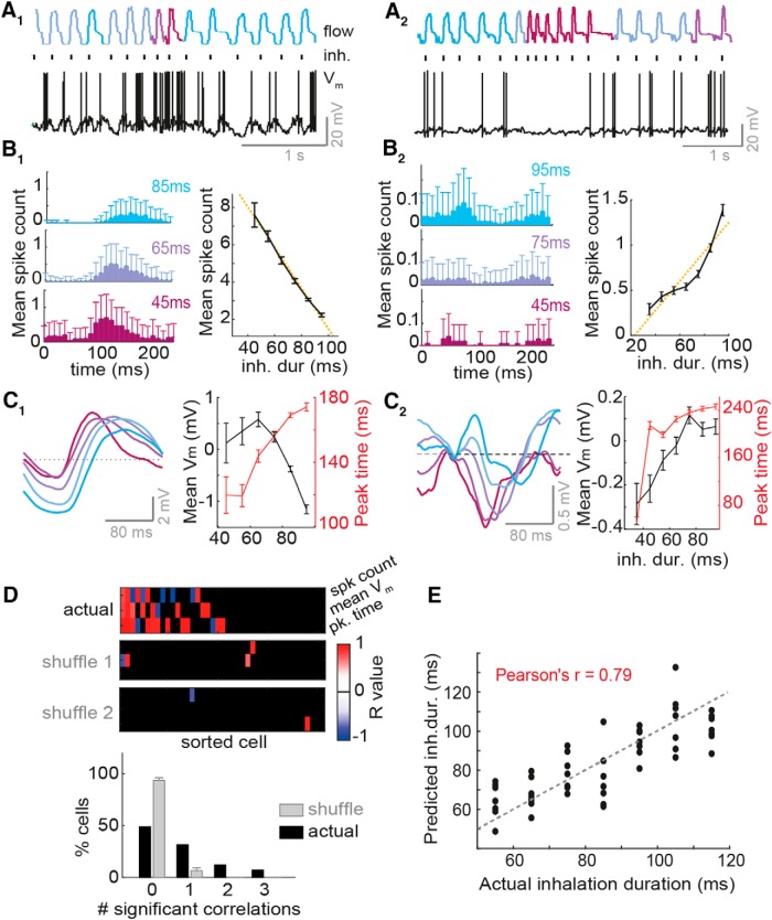
Figure 5.

Inhalation duration transforms mean baseline MTC activity in a large proportion of cells. A₁–C₁ refer to one example cell, while A₂–C₂ refer to a different example cell. A_1–2, Example nasal flow traces and V_m traces in absence of odor. Sniffs are color coded according to inhalation duration (blue = slow, and red = fast). Black ticks indicate inhalation onset. B_1–2, Left: average spike count histograms triggered by inhalations of different durations (denoted on each histogram). Right: mean spike count per sniff as a function of inhalation duration. Error bars = standard error (SE). C_1–2, Left: inhalation-triggered mean V_m waveforms for sniff cycles of different inhalation duration. Right: mean V_m and timing of V_m peak for membrane potential waveforms averaged across all sniffs as a function of inhalation duration. Error bars = SE. D, Top: heatmap of R values for correlations between inhalation duration and 3 different activity parameters (spike count, mean membrane potential, and timing of peak membrane potential, rows 1–3, respectively), for 45 MTCs. Cells are sorted left to right from largest number of significant correlations to lowest number. Black squares show where the correlation was insignificant (p > 0.01, linear regression). Two lowest heatmaps show the same data but for two example shuffle controls, where inhalation durations were shuffled with respect to the physiology, and the data reanalyzed. This gives an indication of false-positive rates in this analysis. Bottom: histogram to show proportion of cells with 0–3 significant correlations between the different activity parameters and inhalation duration. Gray shows proportion for shuffle controls. E, Scatter plot between inhalation duration predicted by a simple linear model using peak spike rates of 25 cells (see Methods) and the actual (true) inhalation duration for all 7 sniff cycles tested in each category. See Fig. 5-1 for the impact of cell type on responses to inhalation change, Fig. 5-2 for further analysis regarding detecting inhalation change, and Fig. 5-3 for a hypothetical relative timing code using this information to infer environmental concentration change.