On the Design and Control of Highly Backdrivable Lower-Limb Exoskeletons: A Discussion of Past and Ongoing Work

Introduction

Lower-limb exoskeletons are external mechanical structures that support and assist human users during locomotion. The earliest studies on exoskeletons date back to the 1960s, whereas over the previous decade, research on powered lower-limb exoskeletons has substantially expanded [1]. Exoskeletons with different architectures have been developed to achieve different goals. Typically, lower-limb exoskeletons can be classified into two broad categories based on their intended use: assisting people who have pathological gaits and augmenting able-bodied users. The first type of exoskeleton is designed to provide assistance to individuals with neurological conditions, for example, stroke or spinal cord injury (SCI). With the help of an exoskeleton, these people can complete different tasks that they cannot complete on their own. For example, the bilateral hip-knee exoskeletons ReWalk [2] and Ekso Bionics [3] enforce pre-defined reference trajectories determined by a finite-state-machine (FSM) structure to assist individuals with SCI. The bilateral Wandercraft exoskeleton adopts a hybrid dynamics-based controller to stabilize dynamically feasible periodic gaits for users with SCI while allowing them to actively control the exoskeleton speed through upper body posture [4].

The second type of exoskeleton is mainly used by able-bodied users for carrying heavy gear and operating cumbersome tools. The majority of these devices transmit force to the ground while tracking a desired reference torque. The Berkeley Lower Extremity Exoskeleton (BLEEX) allows soldiers to carry heavy loads by using its actuators to minimize the interaction forces between the device and the user [5]. The Sarcos-Raytheon “XOS” exoskeleton and the Human Universal Load Carrier (HULC) exoskeletons are also military-based devices aimed at soldier performance enhancement [1]. The soft exosuits presented in [6] can reduce the net metabolic rate for able-bodied subjects during walking by generating assistance through an off-board actuation system and Bowden cables. With advancements in hardware and micro-controller design, an increasing number of complex control algorithms are being realized in practice to promote the rapid development of powered lower-limb exoskeletons.

The majority of assistive exoskeletons are designed to rigidly track time-based kinematic patterns, which forces users to follow specific joint positions during walking. The ReWalk and Ekso Bionics exoskeletons (as well as some other devices [7]–[12]) employ high-ratio transmissions, for example, ball screws or harmonic drives, to achieve the high torques required to track lower-limb kinematics. These rigid actuators are ideal for position-based control methods, as human torques or external force perturbations cannot easily rotate these actuators. Despite the fact that these systems have shown promising results in assisting individuals with SCI, their kinematic control approaches are limited to replicating the normative joint kinematics associated with one specific task and user at a time [1]. These pre-defined trajectories cannot adjust to continuously varying activities or changes in user behavior associated with learning during gait rehabilitation. This control approach must also recognize the user’s intent to transition from one task-specific controller to another [2], [13], which is hard to realize in practice [14]. Multiple task-specific controllers also require more tuning time for each user [15], [16]. Moreover, rigid position control methods require little or no contribution from the human user [17]. This may make sense for people with SCI but not for individuals who have partial or full volitional control of their limbs. For example, individuals post stroke should be allowed to adjust their joint kinematics during the learning process based on corrections from the therapist. Unfortunately, high-ratio transmissions have high mechanical impedance, which prevents users from moving their joints freely without help from the exoskeleton. Individuals with volitional control of their lower extremities require novel design and control methods for exoskeletons that are more compatible with human interaction.

A necessary requirement for assisting or augmenting volitional human motion is for the exoskeleton joints to have low mechanical impedance (that is, backdrivable or “mechanically transparent”). An exoskeleton is said to be backdrivable if users can drive their joints without a high resistive torque from the exoskeleton. This has been achieved in various ways in the past. Active force control attempts to zero the interaction forces measured by a load cell to make the exoskeleton move with the human [5], but this approach has limited bandwidth that prevents more dynamic motions and cannot absorb impact forces [18], [19]. Although the Indego exoskeleton was originally designed for persons with SCI [20], its backdrivable electromechanical actuators have facilitated experiments with individuals post stroke by providing gravity compensation to the swing leg and user/task-specific feedforward movement assistance [13]. The powered knee orthosis in [21] uses a hydraulic actuator to achieve great backdrivability without sacrificing output torque, but electric motors tend to be several times more efficient than hydraulic actuators [18], [22]. Devices with Series Elastic Actuators (SEAs) can realize active backdrivability by servoing the spring displacement to zero, but major limitations still exist such as low output torque [23], [24], complex system architecture [25], [26], and limited force/torque control bandwidth [24], [27]. Soft exosuits [28] by design have low joint impedance, but the control problem becomes substantially harder due to uncertainty in the actuation model from transferring forces to the body through soft, compliant material rather than a rigid structure. Recently, the field of legged robots has started embracing direct-drive and quasi-direct-drive actuation systems (for example, [18], [19], [29]) to enable low-impedance actuation for highly dynamic motions, compliance to impacts, and accurate torque control. We propose that this design philosophy can also be applied in rehabilitation robots to provide users with a cooperative human-machine interface. Having low-impedance actuation also allows the implementation of novel human-interactive control strategies, making it possible for promoting user participation and thus broadening the scope of application for these devices.

Low-impedance actuation is necessary but not sufficient for designing human-interactive exoskeletons, because traditional kinematic control methods can still command large torques that interfere with the volitional motion of the human. Traditional high-gain position control strategies actively increase the overall impedance of the human and exoskeleton system in closed loop, defeating the purpose of the low-impedance actuator design. Therefore, the final requirement concerns the control strategy, which must provide assistance without overly constraining the user’s joint kinematics. Instead of tracking reference kinematic patterns, kinetic goals (for example, energy or force) can be enforced to provide a flexible learning environment and allow the user to choose their own kinematic patterns. In addition to training flexibility, the control method should be task-invariant to provide consistent assistance that eliminates the need for detecting task transitions. Although some task-invariant controllers have been proposed for amplifying human motion [5], [30] or compensating for exoskeleton mass/inertia [13], [31], these approaches assume that the user has the ability to produce the joint kinematics, which is not the case with weakened limbs. Therefore, we focus on an energetic control approach that shapes the Lagrangian (that is, kinetic minus potential energy) of the human body and exoskeleton in closed loop. This energetic control approach, known as energy shaping, controls the system energy to a specific analytical function of the system state in order to induce different dynamics via the Euler-Lagrange equations [32]. By shaping potential energy, torques can be generated to counteract gravity in the vertical direction. This control action yields so-called body-weight support (BWS), which offloads the perceived weight of the user’s lower extremities and center of mass (COM). Similarly, kinetic energy shaping can reduce the perceived mass and inertia of the human-robot system to generate assistance in all directions of motion. Because this control method augments the joint dynamics rather than tracking joint kinematics, the exoskeleton determines how the joints should move instead of where they move. Therefore, the assistance is invariant of the task and the preferred kinematics of the user.

In this paper, we summarize our previous and ongoing work to demonstrate the design and control philosophy behind task-invariant exoskeletal assistance (see “Summary of the Paper”). We applied the proposed design philosophy to build a powered ankle exoskeleton (Generation Zero) that served as a tethered engineering testbed for preliminary experiments [33]. We then present the design of a mobile powered knee-ankle exoskeleton (Generation One) using a high torque-density electrical motor and a custom low-ratio transmission [34], which can achieve high torque output without sacrificing intrinsic backdrivability or efficiency. To control these exoskeletons in a human-cooperative manner, we propose a complete theoretical framework for underactuated energy shaping that incorporates both environmental and human interaction [35]–[37]. By explicitly modeling holonomic contact constraints in the dynamics, we transform the conventional Lagrangian dynamics into the equivalent constrained dynamics (ECD) that have fewer (or possibly zero) unactuated degrees of freedom (DOFs). These constrained dynamics ease the solving of the matching conditions, which determine what energetic properties of the human body can be shaped by the available actuators. This theoretical framework can accommodate arbitrary degrees of underactuation and system dimensions, and the resulting control law can assist any task by augmenting body energetics rather than tracking reference trajectories.

The rest of the paper is organized as follows. In the following section, we introduce the design philosophy for highly backdrivable actuation systems and present the mechatronic and electrical design for two generations of exoskeletons. Then we derive the generalized matching framework for energy shaping with environmental and human interaction. We show simulation results for different shaping strategies on an 8-DOF human-like biped. Finally, able-bodied human subject experiments demonstrate the backdrivability of the powered knee-ankle exoskeleton and validate the potential energy shaping control strategy across a variety of locomotor tasks.

Design of Highly Backdrivable Exoskeletons

In this section, we present the mechatronic designs for two generations of powered exoskeletons shown in Figure 1. The required high torque output of these devices are achieved by increasing the torque density of the electrical motor rather than the transmission ratio. The reflected inertia (or mechanical impedance) of these actuators is drastically reduced through the use of a low-ratio transmission. This actuation design is capable of controlling the output torque without any torque sensing, because direct-drive and quasi-direct-drive actuation systems can be modeled as linear systems [38]. These designs are also intrinsically backdrivable (without any sensing or control), which is ideal for human interaction. Moreover, low-impedance actuators have the potential for energy regeneration during periods of negative work [18], which helps to extend battery life or choose smaller batteries.

Figure 1.

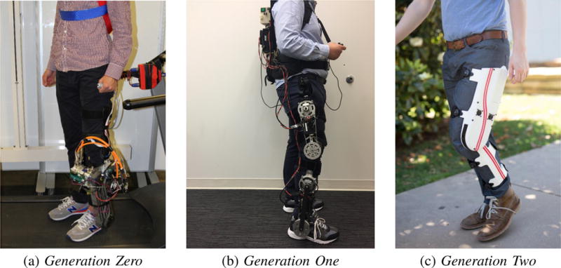
Three generations of exoskeleton prototypes: the Powered Ankle Exoskeleton (left, Generation Zero, image reproduced from [33]), the Powered Knee-Ankle Exoskeleton (center, Generation One), and the Powered Knee Exoskeleton (right, Generation Two). All prototypes are designed with a combination of high-torque motors and low-ratio transmissions.

Generation Zero: Powered Ankle Exoskeleton

As the first step in design, we built a powered ankle exoskeleton to validate the proposed design philosophy [33]. The hardware design presented in this section was mainly conducted to achieve high torque output, accurate torque control performance, and low backdrive torque.

To obtain a sufficient torque output and a small torque ripple, we chose a high torque actuator with a permanent magnetic synchronous motor (PMSM) connected to a two-stage planetary gear transmission (TPM 004X, Wittenstein, Inc., 2.4 kg, efficiency 94%). We used another transmission, a poly chain GT Carbon timing belt (8MGT 720, Gates Industry, Inc., efficiency between 92.8% and 97.8%), to further increase actuator output torque and move the heavy weight towards user’s COM, which minimizes the metabolic burden of added weight during locomotion [39]. Given the combined transmission ratio (43.71:1), approximate efficiency (90%), and peak motor torque (1.29 Nm), the actuator’s peak torque and power were estimated to be 50 Nm and 288 W, respectively. The CAD rendering of the ankle exoskeleton design is shown in Figure 2.

Figure 2.

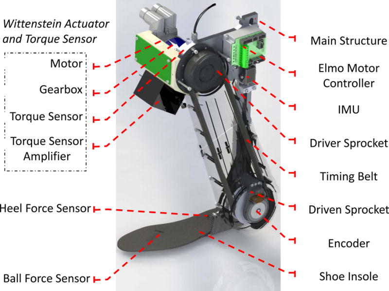
The powered ankle exoskeleton (Generation Zero). This is a single joint exoskeleton that provides an increased output torque to the ankle joint with small torque ripple. This is achieved by combining a permanent magnetic synchronous motor (PMSM) and a two-stage planetary gear transmission with a poly chain GT Carbon timing belt. This figure is reproduced from [33].

For the purpose of control implementation, we measured several features of the human’s walking gait (walking phase, ankle angle, and shank angle) using the following sensors. We placed two force sensors (FlexiForce A301, Tekscan, Inc.) in a custom shoe insole (one under the heel and the other under the ball of the foot) to detect the heel strike, mid-stance, and pre-swing phases of the gait. The insole, made from a rubber-like PolyJet photopolymer, was produced with a Connex 350 3D printer. We measured the ankle angle with an optical incremental encoder (2048 CPR, US Digital, Inc.) and the global orientation of the shank with an inertial measurement unit (IMU) (3DM-GX4-25, LORD MicroStrain, Inc.) on the main structure.

Having designed and built the device, we conducted a torque step response test to verify the performance of the actuation system. We installed a reaction torque sensor (TPM 004+, Wittenstein, Inc.) between the actuator case and main structure to measure the real torque output from the actuator. In this experiment, the actuator was locked in place while we completed a medium torque test (20 Nm) and a high torque test (35 Nm). The results in Figure 3 have a short response time and small steady error. The backdrivability of the device was then demonstrated by treadmill experiments with able-bodied subjects, who walked at various speeds with and without closed-loop torque control [33]. However, the use of industrial components resulted in an overall exoskeleton mass of about 4.5 kg, which was too heavy for a single joint exoskeleton for mobile gait assistance. The tethered power supply and overall size also constrained the device to a stationary treadmill training environment. In the next iteration of our design philosophy, we used custom components to create a next generation powered knee-ankle exoskeleton that is light enough for mobile gait assistance.

Figure 3.

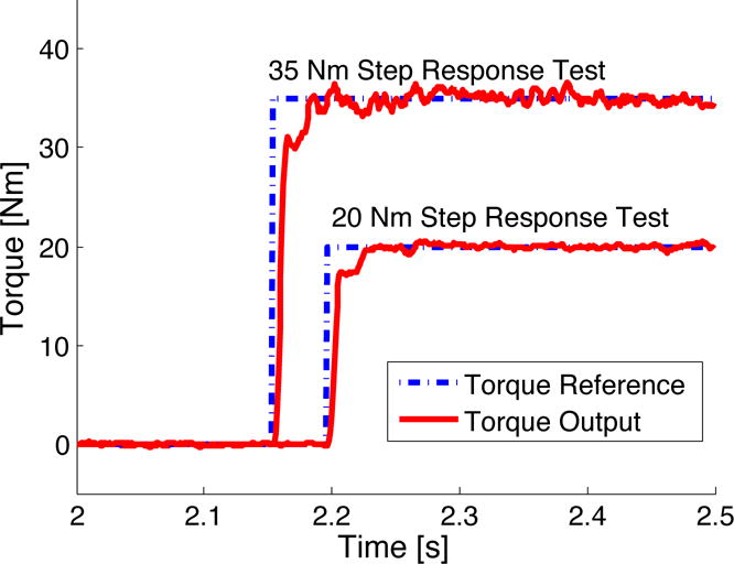
Step response results of the ankle exoskeleton’s actuator. The dashed line indicates the step reference and the solid red line indicates the actual torque output. This test was conducted with a 35 Nm and 20 Nm step reference, respectively. This figure is reproduced from [33].

Generation One: Powered Knee-Ankle Exoskeleton

In this section, we introduce our second exoskeleton prototype: the powered knee-ankle exoskeleton [34] shown in Figure 4. The two actuator modules are attached to a knee-ankle-foot orthotic brace to drive the knee and ankle joints. Torque is transferred to the human ankle through a carbon fiber shoe insert. Several sensors are installed on the brace and the actuator modules to monitor key variables of the gait cycle as shown in the block diagram of Figure 5.

Figure 4.

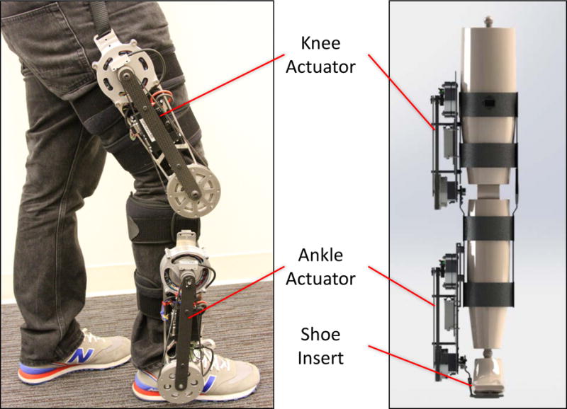
The powered knee-ankle exoskeleton (left) and its rendering (right). Two modular actuators are attached to a knee brace and provide torque to the knee and ankle joints of the affected leg. Torque is transferred to the ankle with the use of a small shoe insert that also houses two small pressure sensors along the Center of Pressure (COP) to aid the control system. This figure is reproduced from [34].

Figure 5.

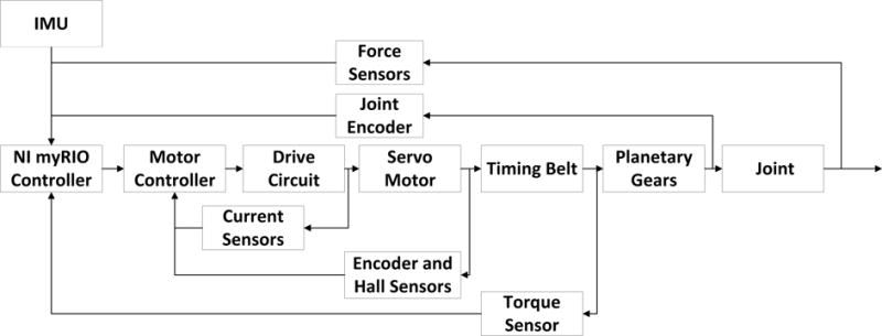
Schematic of the powered knee-ankle exoskeleton system. A servo motor generates a torque, which is then amplified by a timing belt and a planetary gear transmission. Sensor data are fed into a myRIO controller for information processing and commanding the motor controller. This figure is reproduced from [34].

Motors and Transmissions

To reduce the weight and package factor, we used frameless high torque density PMSMs (that is, AC servo motors) and a custom transmission to provide sufficient input torque and power to the user. By optimizing the motor winding configuration, the custom motor (MF0096008, Allied Motion, Inc.) can produce 7.2 Nm peak torque and 200 W power. A distributed two-stage low-ratio transmission was designed for the actuator. We used a poly chain GT carbon timing belt (3MR, Gates Industry, Inc., 4:1 ratio, efficiency between 92.8% and 97.8%) to amplify the motor torque and to move the actuator weight closer to the user’s COM. A custom 6:1 planetary gear transmission (minimum efficiency of 90% [40]) was built inside the driven sprocket of the timing belt to minimize weight and size. The overall ratio of the two-stage transmission was 24:1 with an estimated efficiency between 83.5% and 88%. The schematic of the actuator is shown in Figure 6. In theory, the combination of the torque dense motor and the distributed low-ratio transmission could produce over 150 Nm output torque. However, the motor’s torque was limited by a thermal condition, and the motor’s velocity output was limited by working voltage. To balance the torque and velocity requirements, the actuation system was designed to provide 30 Nm continuous torque output with peak velocity at 80 RPM. The peak torque was limited to 60 Nm by the mechanical structure and the maximum current (30 A) of the motor driver (G-TWI-25/100-SE, Elmo Motion Control, Ltd.).

Figure 6.

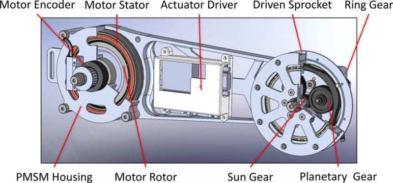
Schematic of the modular actuator of the powered knee-ankle exoskeleton. A frameless electrical motor is integrated with the mechanical structure of the exoskeleton. A timing belt connects the output shaft of the motor to the sun gear. A planetary gear set is built inside the driven sprocket yielding a lightweight, power dense actuator. This figure is reproduced from [34].

Design of Mechanical and Electrical Systems

The frameless motor and custom transmission were integrated into the mechanical structure to further reduce the weight of the exoskeleton. For instance, the motor housing is part of the main structure of the exoskeleton, which was mainly manufactured with aluminum alloy. Several carbon fiber pieces were used to reduce heavy metal materials and strengthen the actuation system. The final mass of each module (knee versus ankle) was about 2 kg with detailed specifications given in Table 1. Considering only actuator components, the torque density of each actuator is about 50 Nm/kg. The total mass of this exoskeleton is similar to our first prototype (Generation Zero) but includes two actuators instead of only one at the ankle. The package factor and mass characteristics were greatly improved by using frameless components.

TABLE 1.

Mass specifications of the powered knee-ankle exoskeleton. Note that the knee and ankle modules include the mass of onboard electronics and cabling.

Components	Mass [kg]
Knee module (thigh)	2.106
Ankle module (shank)	1.843
Shoe insert	0.356
Thigh attachment	0.632
Shank attachment	0.471
Total mass	5.41

The electrical system of this exoskeleton has two main parts: a high-level gait control system and a low-level actuator drive system. The gait control system monitors the key variables of the user’s gait to implement any given torque-based rehabilitation control algorithm. The actuator drive system tracks torque commands from the gait control system as shown in the block diagram of Figure 7.

Figure 7.

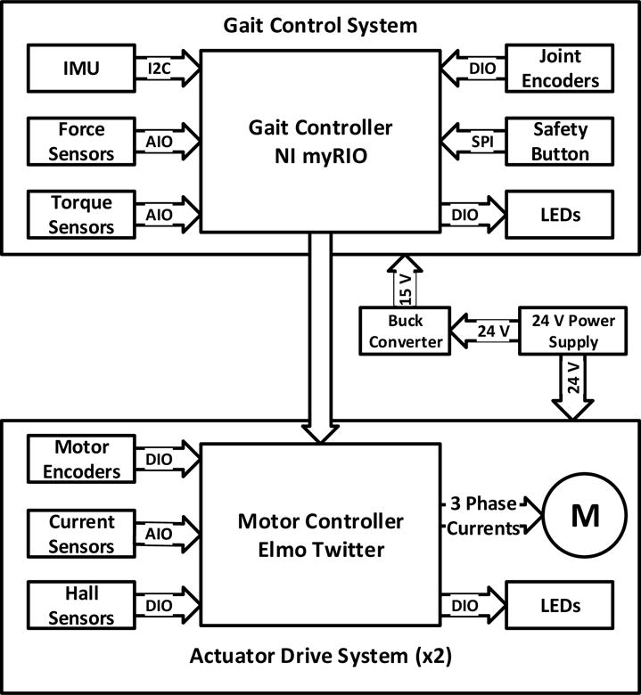
Block diagram of the electrical system of the powered knee-ankle exoskeleton: the gait control system receives feedback related to the user’s gait and sends torque commands. The two actuator drive systems control and drive the knee and ankle actuators. A buck DC-DC converter provides power to the gait control system. This figure is reproduced from [34].

Torque Control System

A common method for controlling torque is based on estimating the actuator’s output torque through the motor phase currents, the transmission ratio ξ, and efficiency η. The actuator output torque T_a and the electromagnetic motor torque T_e are given by

$$T_a=T_e\xi \eta =\left(3P/2\right){\lambda }_m{I}_q\xi \eta ,$$ (1)

where P is the number of motor poles, λ_m is the motor flux linkage, I_q is the active current in the d-q rotating reference frame calculated by the Clarke and Park transformations [41]. Equation (1) determines the reference motor current to achieve the desired output torque, and the motor driver regulates the motor current using a Proportional-Integral (PI) controller in the inner loop of Figure 8. This low-level current loop operates at a much higher sampling rate than the gait control system (approximately 10 kHz versus 1 kHz, respectively), so their dynamics are separately controlled.

Figure 8.

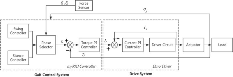
Torque control system schematic, where q_j represents joint angles, F₁ and F₂ are ground reaction forces, T_r is the reference torque, T_f is the measured output torque, I_r is the reference current, and I_q is the motor’s active current [41]. The phase selector switches between the stance and swing controllers, which produce the torque references. The actuator drive system contains two PI control loops. The inner loop is the current PI controller which regulates the motor’s current. The outer loop is the torque PI controller to compensate for the actuator’s torque tracking error. This figure is reproduced from [34].

The accuracy of the torque output via equation (1) depends on a known transmission efficiency η, which can vary during dynamic motion due to different factors such as asymmetric friction loss [42]. A potential benefit of a low-ratio transmission is that the efficiency is higher and more constant (for example, fewer gears meshing [40], [43]) and thus improves the accuracy of current-based torque control [18]. To demonstrate this by comparison, we implemented a second (outer) torque control loop to compensate the torque error measured by a reaction torque sensor (M2210E, Sunrise Instruments Co., Ltd.) inline between the actuator and joint. Both loops (inner current loop and outer torque loop) use PI control to enforce the torque commanded by the higher-level joint control strategy. The overall control schematic is shown in Figure 8.

Benchtop Tests

Before testing the exoskeleton on human subjects, we conducted benchtop tests to characterize the actuator’s performance. We first measured the static backdrive torque, which is defined as the minimum torque required to overcome static friction to backdrive the actuator. A torque was manually applied to the output shaft of the actuator and gradually increased until rotation began. At this point the actuator’s inline reaction torque sensor measured 1.5 Nm. The backdrive torque during dynamic conditions will be reported through treadmill walking tests in the human subject experiments section.

We also conducted a high torque test to verify the actuator’s torque output and the related response time. The actuator was mounted to a testing platform and its output shaft was mechanically fixed. Then, a low torque of 3 Nm was set to preload the actuator and ensure that any mechanical backlash would not interfere with the test. Finally, a torque of 50 Nm was commanded, maintained for 5 seconds, and then set back to zero. The results of this test are plotted in Figure 9. Once the system had settled (t ≥ 0.4 in Figure 9(a)), the steady state error was less than 1.3%. These test results were imported into Matlab Control and Simulation Toolbox and used to generate a model of the system. This model suggests that the system’s torque bandwidth is 10 Hz, which exceeds the required bandwidth for human walking (4-8 Hz [44]).

Figure 9.

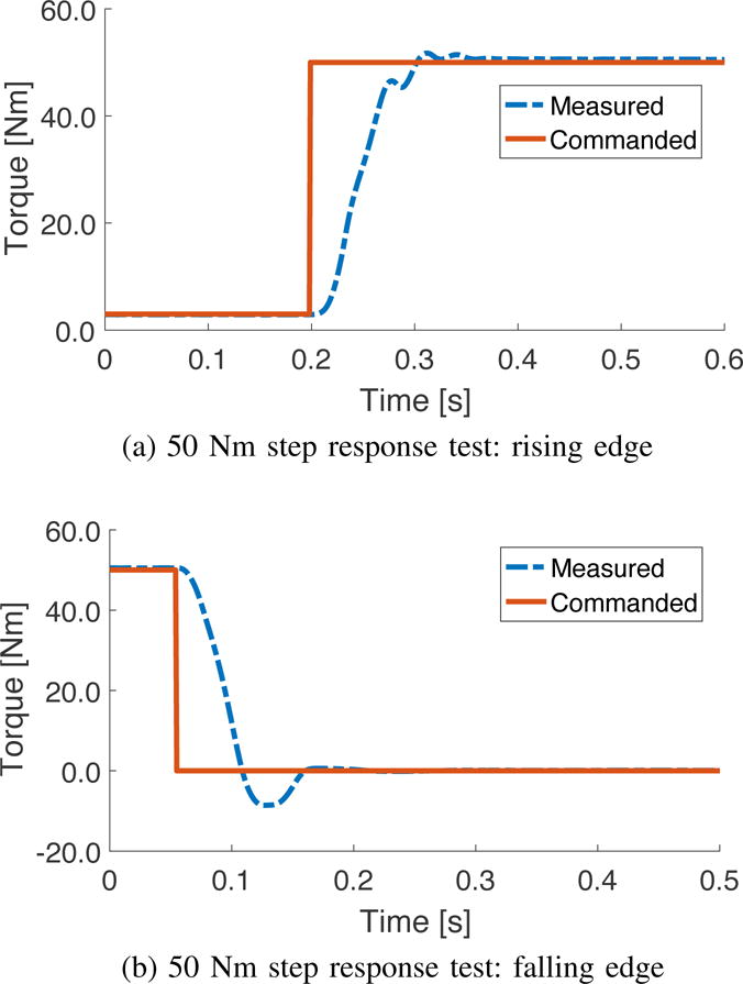
Results from static torque test. The top and bottom figures show the rising and falling edges of a 50 Nm torque step response. Note that the rising edge started from a pretension of 3 Nm.

Summary

This design philosophy successfully balances the core requirements of volitional gait assistance: backdrivability, torque-based control, high torque density, and light weight. High output torque is achieved by increasing the torque density of the electrical motor rather than increasing the transmission ratio. This low-ratio actuator design provides intrinsic backdrivability without the high cost and complexity of variable transmissions, clutches, and/or series elastic components. Our second-generation powered knee exoskeleton (Figure 1, right) takes this design philosophy further with a lower transmission ratio (7:1 via one-stage planetary gears), which is discussed in the future work section.

Energy Shaping Control of Lower-Limb Exoskeletons

Conventional trajectory-based control tends to give the user the least amount of volitional control over the device, which limits its applicability to different patient populations [45]. Instead of tracking kinematic trajectories, this section will introduce a task-invariant, energetic control approach for providing exoskeletal assistance known as energy shaping. Energy shaping has been applied to biped models to facilitate natural, efficient gaits [46]–[49] based on passive dynamics. Although promising results have been shown, these works have been limited to simple toy models where the matching conditions (to be introduced later) are tractable. Similarly, these biped models have point feet or flat feet with a single contact model, often assuming full actuation. Humans are not point-footed or flat-footed walkers. In human walking, contact varies from heel to toe resulting in multiple periods of underactuation, which cannot be captured by the existing framework. It is also unknown how to incorporate human interaction. Therefore, in this section we propose a complete theoretical framework for underactuated energy shaping that incorporates both environmental and human interaction.

Energy Shaping: A Brief Review

Energy shaping is a control method that alters the dynamical characteristics of a mechanical system [50]–[54]. In this part we briefly review the traditional concept of energy shaping. Consider a forced n-dimensional Euler-Lagrange system with configuration space ℚ (assume ℝⁿ for simplicity) and its tangent bundle Tℚ = ⋃_q∈ℚT_qℚ. We can describe the system by a Lagrangian $\mathcal{L}\left(q,\dot{q}\right)$ defined as

$$\mathcal{L}\left(q,\dot{q}\right)=\mathcal{K}\left(q,\dot{q}\right)-\mathcal{P}\left(q\right)=\frac{1}{2}{\dot{q}}^{T}M\left(q\right)\dot{q}-\mathcal{P}\left(q\right),$$ (2)

where the Lagrangian $\mathcal{L}\left(q,\dot{q}\right):T\mathrm{\mathbb{Q}}\to \mathrm{ℝ}$ is a smooth function, q ∈ ℚ is the generalized coordinates vector, and $\dot{q}\in T_q\mathrm{\mathbb{Q}}$ is the velocity vector. The scalar function $\mathcal{K}\left(q,\dot{q}\right):T\mathrm{\mathbb{Q}}\to \mathrm{ℝ}$ is the kinetic energy defined based on the positive-definite mass/inertia matrix M(q) ∈ ℝ^n×n, and $\mathcal{P}\left(q\right):\mathrm{\mathbb{Q}}\to \mathrm{ℝ}$ is the potential energy. The Lagrangian dynamics are given by

$$\frac{d}{dt}{\partial }_{\dot{q}}\mathcal{L}\left(q,\dot{q}\right)-{\partial }_q\mathcal{L}\left(q,\dot{q}\right)=\tau ,$$ (3)

which can be further expressed as

$$M\left(q\right)\ddot{q}+C\left(q,\dot{q}\right)\dot{q}+N\left(q\right)=\tau ,$$ (4)

where $C\left(q,\dot{q}\right)\in {\mathrm{ℝ}}^{n\times n}$ is the Coriolis/centrifugal matrix, $N\left(q\right)={\nabla }_q\mathcal{P}\left(q\right)\in {\mathrm{ℝ}}^n$ is the gravitational forces vector, and τ ∈ ℝⁿ contains all external (nonconservative) forces. For the underactuated case, τ = B(q)u where matrix B(q) ∈ ℝ^n×p maps the control input u ∈ ℝ^p to the n-dimensional dynamics (n > p).

Now consider an unforced Euler-Lagrange system defined by another Lagrangian $\stackrel{\sim }{\mathcal{L}}\left(q,\dot{q}\right):T\mathrm{\mathbb{Q}}\to \mathrm{ℝ}$ described as

$$\stackrel{\sim }{\mathcal{L}}\left(q,\dot{q}\right)=\stackrel{\sim }{\mathcal{K}}\left(q,\dot{q}\right)-\stackrel{\sim }{\mathcal{P}}\left(q\right)=\frac{1}{2}{\dot{q}}^T\stackrel{\sim }{M}\left(q\right)\dot{q}-\stackrel{\sim }{\mathcal{P}}\left(q\right)$$ (5)

with a new kinetic energy $\stackrel{\sim }{\mathcal{K}}\left(q,\dot{q}\right):T\mathrm{\mathbb{Q}}\to \mathrm{ℝ}$ and a new potential energy $\stackrel{\sim }{\mathcal{P}}\left(q\right):\mathrm{\mathbb{Q}}\to \mathrm{ℝ}$. The resulting Lagrangian dynamics can be expressed as

$$\frac{d}{dt}{\partial }_{\dot{q}}\stackrel{\sim }{\mathcal{L}}\left(q,\dot{q}\right)-{\partial }_q\stackrel{\sim }{\mathcal{L}}\left(q,\dot{q}\right)=0$$ (6)

which can be also expressed as

$$\stackrel{\sim }{M}\left(q\right)\ddot{q}+\stackrel{\sim }{C}\left(q,\dot{q}\right)\dot{q}+\stackrel{\sim }{N}\left(q\right)=0,$$ (7)

where $\stackrel{\sim }{C}\left(q,\dot{q}\right)$ is the Coriolis/centrifugal matrix in closed loop, and $\stackrel{\sim }{N}\left(q\right)={\nabla }_q\stackrel{\sim }{\mathcal{P}}\left(q\right)$.

We say the systems (4) and (7) match if (7) is a possible closed-loop system of (4), that is, there exists a control law u such that (4) becomes (7). Equivalently, standard results in [52] shows that these two system match if and only if there exists a full-rank left annihilator B(q)^⊥ ∈ ℝ^{(n − p)×n} of B(q), that is, B(q)^⊥B(q) = 0 and rank(B(q)^⊥) = n − p, ∀q ∈ ℚ, such that

$$B^{\perp }\left(q\right)\left[C\left(q,\dot{q}\right)\dot{q}+N\left(q\right)-M\left(q\right)\stackrel{\sim }{M}{\left(q\right)}^{-1}\left(\stackrel{\sim }{C}\left(q,\dot{q}\right)\dot{q}+\stackrel{\sim }{N}\left(q\right)\right)\right]=0.$$ (8)

Equation (8) is the so-called matching condition, which is a nonlinear partial differential equation that determines the achievable closed-loop energy. Assuming (8) is satisfied, one can obtain that

$$B\left(q\right)u=M\left(q\right)\ddot{q}+C\left(q,\dot{q}\right)\dot{q}+N\left(q\right)-\left(\stackrel{\sim }{M}\left(q\right)\ddot{q}+\stackrel{\sim }{C}\left(q,\dot{q}\right)\dot{q}+\stackrel{\sim }{N}\left(q\right)\right).$$ (9)

Solving (7) for $\ddot{q}$, one can obtain the expression as

$$\ddot{q}=-\stackrel{\sim }{M}{\left(q\right)}^{-1}\left(\stackrel{\sim }{C}\left(q,\dot{q}\right)\dot{q}+\stackrel{\sim }{N}\left(q\right)\right).$$ (10)

Substituting (10) into (9) and multiplying the left-pseudo inverse of B(q) (equivalent to matrix inverse for n = p) on both sides of (9), one obtains the control law as [32]

$$u={\left(B{\left(q\right)}^{T}B\left(q\right)\right)}^{-1}B{\left(q\right)}^T\left[C\left(q,\dot{q}\right)\dot{q}+N\left(q\right)-M\left(q\right)\stackrel{\sim }{M}{\left(q\right)}^{-1}\left(\stackrel{\sim }{C}\left(q,\dot{q}\right)\dot{q}+\stackrel{\sim }{N}\left(q\right)\right)\right].$$ (11)

Interacting with the Environment

The matching condition (8) is trivially satisfied for all $\stackrel{\sim }{M}\left(q\right)$ and $\stackrel{\sim }{\mathcal{P}}\left(q\right)$ if n = p, that is, if the system is fully-actuated [32]. When the system is underactuated (n > p), solutions of the matching condition become quite difficult to obtain [55]. Contact constraints affect the number of unactuated coordinates and therefore must be considered when deriving energy-shaping control laws. In this part, we present generalized dynamics with contact constraints and derive the corresponding matching conditions. To begin, we model a planar biped that combines the human body and exoskeleton(s). For simplicity we lump the torso and hip together as a single mass (that is, only one hip joint), but the following framework can also be used with more human-like models.

Modeling the Biped

The biped is modeled as a kinematic chain with respect to an inertial reference frame (IRF, to be specified later) shown in Figure 10. Depending on whether the exoskeleton is unilateral or bilateral, we choose to model the stance and swing legs separately (unilateral case [35], [36]) or the entire lower body as a kinematic chain from the stance foot to the swing foot (bilateral case [37]). By explicitly modeling contact constraints in the dynamics, the EOM can be expressed as

$$M\left(q\right)\ddot{q}+C\left(q,\dot{q}\right)\dot{q}+N\left(q\right)+A{\left(q\right)}^T\lambda =\tau ,$$ (12)

where M(q) ∈ ℝ^n×n, $C\left(q,\dot{q}\right)\in {\mathrm{ℝ}}^{n\times n}$, and N(q) ∈ ℝ^n×1 are defined similar to the terms in (4). The configuration vector is given as $q={\left({\theta }_{\mathrm{x}},{\theta }_{\mathrm{y}},{\theta }_{\text{ab}},q_{\mathrm{s}}^T\right)}^T\in {\mathrm{ℝ}}^n$, where θ_x and θ_y are the Cartesian coordinates with respect to the IRF, θ_ab is an absolute angle defined with respect to the vertical axis, and the shape vector q_s ∈ ℝⁿ⁻³ contains joint angles based on the biped model (to be specified in the simulation section). The matrix A(q)^T ∈ ℝ^n×c is the constraint matrix defined as the gradient of the holonomic constraint functions (see next section), and c is the number of contact constraints depending on the contact condition. The Lagrange multiplier is calculated using the method in [15], [56] as

$$\begin{gathered} \lambda =\widehat{\lambda }+\overline{\lambda }\tau ,\text{where} \\ \lambda =W\left(q\right)\left(\dot{A}\left(q\right)\dot{q}-A\left(q\right)M{\left(q\right)}^{-1}C\left(q,\dot{q}\right)\dot{q}-A\left(q\right)M{\left(q\right)}^{-1}N\left(q\right)\right), \\ \overline{\lambda }=W\left(q\right)A\left(q\right)M{\left(q\right)}^{-1},\text{where} \\ W\left(q\right)={\left(A\left(q\right)M{\left(q\right)}^{-1}A{\left(q\right)}^T\right)}^{-1}. \end{gathered}$$ (13)

Because we are lumping the human body and exoskeleton together, the torque τ = τ_hum + τ_exo at the right-hand side of (12) comprises the human input terms τ_hum = B(q)v + J(q)^T F and the exoskeleton input τ_exo = B(q)u. The mapping matrix B(q) ∈ ℝ^n×p maps both the human muscular torques v ∈ ℝ^p and the exoskeleton actuator torques u ∈ ℝ^p into the dynamics. Without loss of generality, we assume B(q) takes the form of [0_p×(n−p), I_p×p]^T. The force vector F = (F_x, F_y, M_z)^T ∈ ℝ^3×1 in τ_hum denotes the interaction forces between the stance model and the swing leg model, where (F_x, F_y)^T and M_z indicate the two linear forces and a moment in the sagittal plane, respectively. The forces F are mapped into the dynamics by the body Jacobian matrix J(q)^T ∈ ℝ^n×3. Note that for bilateral exoskeleton models, the interaction forces F are internal to the dynamics of the complete kinematic chain and hence will not show up as an external input (that is, F = 0).

Figure 10.

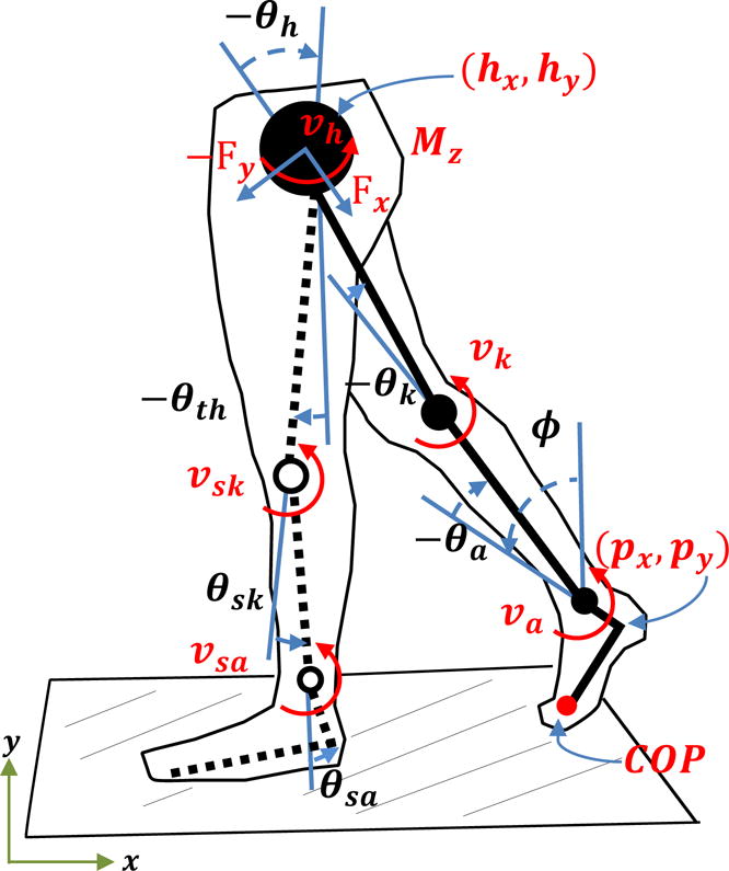
Kinematic model of the human body and the exoskeleton(s). The stance leg is shown in solid black and the swing leg (just before impact) in dashed black. For controlling a unilateral exoskeleton, we separately model the stance and swing legs. The stance leg is modeled as a kinematic chain from the inertia reference frame (IRF), which is defined at the stance heel during heel and flat foot contact versus the stance toe during toe contact. As for the swing leg, we choose the hip as a floating base for the swing leg’s kinematic chain. The forces F = (F_x, F_y, M_z)^T ∈ ℝ^3×1 are the interaction forces between the hip of the stance model and the swing thigh. For modeling a human wearing a bilateral exoskeleton, we combine the stance and swing leg models (full biped model) and the forces F are implicitly modeled in the equations of motion (EOM) of the complete kinematic chain. For simulations of the full biped model, the angle θ_h is defined as the hip angle between the stance and swing thighs, and the red arcs indicate the human muscle inputs.

Holonomic Contact Constraints

In the previous section, we explicitly modeled contact in the dynamics without specifying the choice of contact constraints. In this section, we define the general form of holonomic contact constraints encountered during the single-support period of human walking, which are expressed as relations between the position variables:

$$a\left(q_1,q_2,\dots ,q_c\right)=0_{c\times 1},$$ (14)

where q_i denotes the i-th element of the configuration vector q. The single-support period can be separated into heel contact, flat foot, and toe contact phases, based on which appropriate holonomic contact constraints can be defined as in Figure 11. There are c = 2 constraints for heel contact and toe contact whereas flat foot has c = 3. We will later show that the proposed framework is able to accommodate arbitrary numbers of contact constraints. In this paper, we assume the constraint matrix A(q) has the constant form

$$A\left(q\right)={\nabla }_{q}a\left(q_1,q_2,\dots ,q_c\right)=\left[I_{c\times c}{0}_{c\times \left(n-c\right)}\right].$$ (15)

This constant form (that is, Ȧ = 0) can be achieved by defining the IRF at the stance toe during toe contact and the stance heel during heel and flat foot contact.

Figure 11.

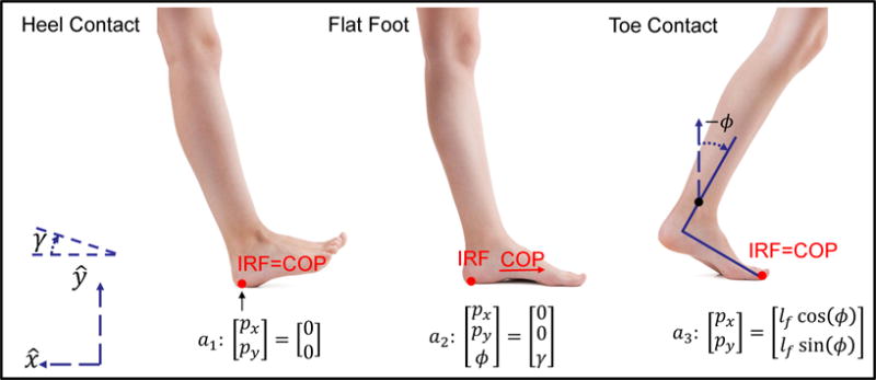
Heel contact configuration (left), flat foot configuration (center), toe contact configuration (right) during the single-support period of human locomotion. For simulation purposes, we assume the biped is walking on a slope with angle γ. To have a constant constraint matrix A, the inertial reference frame (IRF) can be moved to the toe during toe contact, that is, (t_x, t_y)^T = (p_x – l_f cos(ϕ), p_y − l_f sin(ϕ))^T = (0, 0)^T, where (t_x, t_y)^T denotes the position of the toe.

Equivalent Constrained Dynamics

The classical matching condition (8) and control law (11) in the previous subsection cannot be directly applied to the generalized dynamics (12). Although a dynamical system in the form of (4) could be separately modeled for each phase by dropping constrained coordinates from the generalized coordinate vector, this would require a clever change of coordinates for some constraints (for example, rolling contact [57]). The dimension and degree of underactuation of the resulting hybrid system also changes between phases, requiring different models for control law (11). Switching between control models in real time requires precise estimates of gait cycle phase, which can be difficult to achieve in practice [14].

Instead of modeling a different dynamical system for each phase, we will extend the results of the previous sections to a single generalized system (12) to obtain a shaping framework which can accommodate any holonomic contact constraints (and the resulting unactuated DOFs) that could occur during various locomotor tasks. This generalized framework shows what terms can and cannot be shaped with each contact constraint. We start the proposed approach by plugging expressions for A(q) and λ into (12) to obtain the form of (4), which is denoted as the equivalent constrained dynamics that have fewer (possibly zero) unactuated DOFs compared to the generalized dynamics (12) without constraints. From now on, we omit q and $\dot{q}$ in the dynamical terms to abbreviate notations. Following the procedure in [37], the equivalent constrained form of (12) is expressed as

$$M_{\lambda }\ddot{q}+C_{\lambda }\dot{q}+N_{\lambda }=B_{\lambda }v+J_{\lambda }^{T}F+B_{\lambda }u,$$ (16)

$$\begin{gathered} \mathrm{where}{M}_{\lambda }=M, \\ {C}_{\lambda }=\left(I-A^{T}WA{M}^{-1}\right)C+\bcancel{A^{T}W\dot{A}}, \\ {N}_{\lambda }=\left(I-A^{T}WA{M}^{-1}\right)N, \\ {B}_{\lambda }=\left(I-A^{T}WA{M}^{-1}\right)B, \\ {J}_{\lambda }^T=\left(I-A^{T}WA{M}^{-1}\right)J^T. \end{gathered}$$ (17)

Given the open-loop dynamics (16), we define the desired closed-loop ECD as

$${\stackrel{\sim }{M}}_{\lambda }\ddot{q}+{\stackrel{\sim }{C}}_{\lambda }\dot{q}+{\stackrel{\sim }{N}}_{\lambda }={\stackrel{\sim }{\tau }}_{\text{hum}},$$ (18)

where ${\stackrel{\sim }{M}}_{\lambda }=\stackrel{\sim }{M}$ is the mass/inertia matrix in the closed-loop ECD and is assumed to be positive-definite. The remaining terms in (18) are given by

$$\begin{gathered} {\stackrel{\sim }{C}}_{\lambda }=\left(I-A^T\stackrel{\sim }{W}A{\stackrel{\sim }{M}}^{-1}\right)\stackrel{\sim }{C}+\bcancel{A^T\stackrel{\sim }{W}\dot{A}}, \\ {\stackrel{\sim }{N}}_{\lambda }=\left(I-A^T\stackrel{\sim }{W}A{\stackrel{\sim }{M}}^{-1}\right)\stackrel{\sim }{N}, \\ {\stackrel{\sim }{B}}_{\lambda }=\left(I-A^T\stackrel{\sim }{W}A{\stackrel{\sim }{M}}^{-1}\right)\stackrel{\sim }{B}, \\ {\stackrel{\sim }{J}}_{\lambda }^T=\left(I-A^T\stackrel{\sim }{W}A{\stackrel{\sim }{M}}^{-1}\right){\stackrel{\sim }{J}}^T, \\ \stackrel{\sim }{W}={\left(A{\stackrel{\sim }{M}}^{-1}{A}^T\right)}^{-1}, \end{gathered}$$ (19)

where $\stackrel{\sim }{C}$ and Ñ are the dynamics terms of (12) in closed loop. We denote the closed-loop human input vector as ${\stackrel{\sim }{\tau }}_{\text{hum}}={\stackrel{\sim }{B}}_{\lambda }v+{\stackrel{\sim }{J}}_{\lambda }^{T}F$ but make no assumptions on the human inputs v and F. Instead, we assume these two terms are mapped into the closed-loop dynamics by ${\stackrel{\sim }{B}}_{\lambda }$ and ${\stackrel{\sim }{J}}_{\lambda }^T$ with specific choices of $\stackrel{\sim }{B}$ and ${\stackrel{\sim }{J}}^T$ to be defined next.

Matching Based on Equivalent Constrained Dynamics

We begin this part by introducing the generalized matching condition based on ECD. Given (16) and (18), we follow the procedure from (4) to (8) to derive the matching condition for the ECD as

$$B_{\lambda }^{\perp }\left[M_{\lambda }{\stackrel{\sim }{M}}_{\lambda }^{-1}\left({\stackrel{\sim }{B}}_{\lambda }v+{\stackrel{\sim }{J}}_{\lambda }^{T}F-{\stackrel{\sim }{C}}_{\lambda }\dot{q}-{\stackrel{\sim }{N}}_{\lambda }\right)+C_{\lambda }\dot{q}+N_{\lambda }-B_{\lambda }v-J_{\lambda }^{T}F\right]=0,$$ (20)

which can be separated into sub-matching conditions that correspond to matching for kinetic energy, potential energy, and human inputs, respectively:

$$B_{\lambda }^{\perp }\left(C_{\lambda }\dot{q}-M_{\lambda }{\stackrel{\sim }{M}}_{\lambda }^{-1}{\stackrel{\sim }{C}}_{\lambda }\dot{q}\right)=0,$$ (21)

$$B_{\lambda }^{\perp }\left(N_{\lambda }-M_{\lambda }{\stackrel{\sim }{M}}_{\lambda }^{-1}{\stackrel{\sim }{N}}_{\lambda }\right)=0,$$ (22)

$$B_{\lambda }^{\perp }\left[B_{\lambda }v+J_{\lambda }^{T}F-M_{\lambda }{\stackrel{\sim }{M}}_{\lambda }^{-1}\left({\stackrel{\sim }{B}}_{\lambda }v+{\stackrel{\sim }{J}}_{\lambda }^{T}F\right)\right]=0.$$ (23)

Matching for Kinetic Energy

Prior research showed that the bottom-right submatrix of a mass matrix is the mass matrix of a lower-dimensional mechanical system [58]. This motivates us to shape the bottom-right part in M_λ, which may render matching conditions that are easier to satisfy. Following the procedure in [35], [36], we decompose M_λ into matrices blocks, that is,

$$M=\left[\begin{array}{ll}{M}_1\hfill & M_2\hfill \\ M_2^T\hfill & M_4\hfill \end{array}\right]=M_{\lambda },$$ (24)

where M₁ ∈ ℝ^c×c, M₂ ∈ ℝ^{c×(n − c)}. We want the bottom-right part to be shaped via control, hence we define the closed-loop inertia matrix as

$$\stackrel{\sim }{M}=\left[\begin{array}{ll}{M}_1\hfill & M_2\hfill \\ M_2^T\hfill & {\stackrel{\sim }{M}}_4\hfill \end{array}\right]={\stackrel{\sim }{M}}_{\lambda },$$ (25)

where the choice of ${\stackrel{\sim }{M}}_4$ will be specified in the following sections.

Note from [32], [55] that we have the relationship between C and M as

$$C\dot{q}=D_q\left(M\dot{q}\right)\dot{q}-\frac{1}{2}{\partial }_q\left({\dot{q}}^{T}M\dot{q}\right),$$ (26)

where D_x(y) is the Jacobian matrix of partial derivatives of vector y with respect to vector x. Because the first c DOFs are constrained, their time-derivatives equal zero so that (26) reduces to

$$C\dot{q}=D_q\left[\begin{array}{l}{M}_2{\dot{q}}_{c+1,n}\hfill \\ M_4{\dot{q}}_{c+1,n}\hfill \end{array}\right]\left[\begin{array}{l}0\hfill \\ {\dot{q}}_{c+1,n}\hfill \end{array}\right]-\frac{1}{2}{\partial }_q\left({\dot{q}}_{c+1,n}^T{M}_4{\dot{q}}_{c+1,n}\right),$$

where the subscript (i, j) indicates rows i through j of a matrix. Note that the submatrix M₄ does not depend on q₁,_c based on the recursively cyclic property in [58], yielding simplified expressions for $C\dot{q}$ and $\stackrel{\sim }{C}\dot{q}$ as

$$C\dot{q}=\left[\begin{array}{c}{\partial }_{q_{c+1,n}}\left(M_2{\dot{q}}_{c+1,n}\right){\dot{q}}_{c+1,n}\\ \mathrm{\Psi }\end{array}\right],$$ (27)

$$\stackrel{\sim }{C}\dot{q}=\left[\begin{array}{c}{\partial }_{q_{c+1,n}}\left(M_2{\dot{q}}_{c+1,n}\right){\dot{q}}_{c+1,n}\\ \stackrel{\sim }{\mathrm{\Psi }}\end{array}\right],$$ (28)

where

$$\mathrm{\Psi }:=\frac{1}{2}{\partial }_{q_{c+1,n}}\left({\dot{q}}_{c+1,n}^T{M}_4{\dot{q}}_{c+1,n}\right)\in {\mathrm{ℝ}}^{\left(n-c\right)\times 1},\stackrel{\sim }{\mathrm{\Psi }}:=\frac{1}{2}{\partial }_{q_{c+1,n}}\left({\dot{q}}_{c+1,n}^T{\stackrel{\sim }{M}}_4{\dot{q}}_{c+1,n}\right)\in {\mathrm{ℝ}}^{\left(n-c\right)\times 1}.$$

Following the same procedure in [36], we calculate [I − A^TW AM⁻¹] in (16) using the blockwise inversion of M and define $\left[I-A^T\stackrel{\sim }{W}A{\stackrel{\sim }{M}}^{-1}\right]$ accordingly as

$$\left[I-A^{T}WA{M}^{-1}\right]=\left[\begin{array}{cc}{0}_{c\times c}& Y\\ 0_{\left(n-c\right)\times c}& I_{\left(n-c\right)\times \left(n-c\right)}\end{array}\right],$$ (29)

$$\left[I-A^T\stackrel{\sim }{W}A{\stackrel{\sim }{M}}^{-1}\right]=\left[\begin{array}{cc}{0}_{c\times c}& \stackrel{\sim }{Y}\\ 0_{\left(n-c\right)\times c}& I_{\left(n-c\right)\times \left(n-c\right)}\end{array}\right],$$ (30)

where $Y=M_2{M}_4^{-1}$ and $\stackrel{\sim }{Y}=M_2{\stackrel{\sim }{M}}_4^{-1}$. Multiplying (29) with (27) and (30) with (28), we obtain

$$C_{\lambda }\dot{q}=\left[\begin{array}{c}Y\mathrm{\Psi }\\ \mathrm{\Psi }\end{array}\right],{\stackrel{\sim }{C}}_{\lambda }\dot{q}=\left[\begin{array}{c}\stackrel{\sim }{Y}\stackrel{\sim }{\mathrm{\Psi }}\\ \stackrel{\sim }{\mathrm{\Psi }}\end{array}\right].$$ (31)

To simplify the multiplication between M_λ and ${\stackrel{\sim }{M}}_{\lambda }^{-1}$, we apply the blockwise inversion method again to obtain

$$M_{\lambda }{\stackrel{\sim }{M}}_{\lambda }^{-1}=\left[\begin{array}{cc}{I}_{c\times c}& 0_{c\times \left(n-c\right)}\\ {\mathrm{\Omega }}_1& {\mathrm{\Omega }}_2\end{array}\right],$$ (32)

where ${\mathrm{\Omega }}_1=\left(I-M_4{\stackrel{\sim }{M}}_4^{-1}\right)M_2^T{\left(M_1-M_2{\stackrel{\sim }{M}}_4^{-1}{M}_2^T\right)}^{-1}\in {\mathrm{ℝ}}^{\left(n-c\right)\times c}$ and ${\mathrm{\Omega }}_2=-{\mathrm{\Omega }}_1\stackrel{\sim }{Y}+M_4{\stackrel{\sim }{M}}_4^{-1}\in {\mathrm{ℝ}}^{\left(n-c\right)\times \left(n-c\right)}$. The matrix B_λ is calculated from (17) and its annihilator $B_{\lambda }^{\perp }$ can be chosen as

$$B_{\lambda }=\left[\begin{array}{c}Y{B}_{c+1,n}\\ B_{c+1,n}\end{array}\right],B_{\lambda }^{\perp }=\left[\begin{array}{cc}{I}_{c\times c}& -Y\\ 0_{\left(n-p-c\right)\times c}& S\end{array}\right],$$ (33)

where S = [I_{(n − p − c)×(n − p − c)}, 0_{(n − p − c)×p}]. When the system is fully-constrained, that is, n = p + c, the second block row of the annihilator disappears. It can be verified that $B_{\lambda }^{\perp }\in {\mathrm{ℝ}}^{\left(n-p\right)\times n}$, $\text{rank}\left(B_{\lambda }^{\perp }\right)=n-p$, and $B_{\lambda }^{\perp }{B}_{\lambda }=0_{\left(n-p\right)\times p}$. Plugging $B_{\lambda }^{\perp }$, (32), and (31) into (21), the left-hand side of the matching condition becomes

$$B_{\lambda }^{\perp }\left[C_{\lambda }\dot{q}-M_{\lambda }{\stackrel{\sim }{M}}_{\lambda }^{-1}{\stackrel{\sim }{C}}_{\lambda }\dot{q}\right]=\left[\begin{array}{cc}{I}_{c\times c}& -Y\\ 0_{\left(n-p-c\right)\times c}& S\end{array}\right]\left[\begin{array}{c}Y\mathrm{\Psi }-\stackrel{\sim }{Y}\stackrel{\sim }{\mathrm{\Psi }}\\ \mathrm{\Psi }-{\mathrm{\Omega }}_1\stackrel{\sim }{Y}\stackrel{\sim }{\mathrm{\Psi }}-{\mathrm{\Omega }}_2\stackrel{\sim }{\mathrm{\Psi }}\end{array}\right].$$ (34)

The first c rows of (34) can be simplified as

$$\begin{array}{l}\left[I_{c\times c}-Y\right]\left[\begin{array}{c}Y\mathrm{\Psi }-\stackrel{\sim }{Y}\stackrel{\sim }{\mathrm{\Psi }}\\ \mathrm{\Psi }-{\mathrm{\Omega }}_1\stackrel{\sim }{Y}\stackrel{\sim }{\mathrm{\Psi }}-{\mathrm{\Omega }}_2\stackrel{\sim }{\mathrm{\Psi }}\end{array}\right]\\ =\left(-\stackrel{\sim }{Y}+Y{\mathrm{\Omega }}_1\stackrel{\sim }{Y}+Y{\mathrm{\Omega }}_2\right)\stackrel{\sim }{\mathrm{\Psi }}=\left(-\stackrel{\sim }{Y}+Y{M}_4{\stackrel{\sim }{M}}_4^{-1}\right)\stackrel{\sim }{\mathrm{\Psi }}\\ =\left(-\stackrel{\sim }{Y}+M_2{\stackrel{\sim }{M}}_4^{-1}\right)\stackrel{\sim }{\mathrm{\Psi }}=0_{c\times 1}.\end{array}$$ (35)

For contacts (for example, heel or toe contact) that result in underactuation (n > p+c), additional analysis is needed to fully satisfy the matching condition (21), that is, the bottom (n − p − c) rows of (34) must also be satisfied.

Note that during underactuated cases, M₄ cannot be shaped arbitrarily. We propose satisfying the matching condition by shaping only the bottom-right p × p part of M₄, which is associated with the p actuated coordinates. To show this, we first decompose and shape M₄ in a similar manner to (25) as

$$M_4=\left[\begin{array}{cc}{M}_{41}& M_{42}\\ M_{42}^T& M_{44}\end{array}\right],{\stackrel{\sim }{M}}_4=\left[\begin{array}{cc}{M}_{41}& M_{42}\\ M_{42}^T& {\stackrel{\sim }{M}}_{44}\end{array}\right],$$

where M₄₁ ∈ ℝ^{(n−p−c)×(n−p−c)}, M₄₂ ∈ ℝ^{(n−p−c)×p}, and M₄₄, ${\stackrel{\sim }{M}}_{44}\in {\mathrm{ℝ}}^{p\times p}$. Similar to (32), the top-left element of $M_4{\stackrel{\sim }{M}}_4^{-1}$ will be I_{(n−p−c)×(n−p−c)}. Subtracting $M_4{\stackrel{\sim }{M}}_4^{-1}$ from I_{(n−c)×(n−c)}, the first (n−p−c) rows of Ω₁ will become zeroes. As a consequence, the first (n−p−c) rows of Ω₂ become [I_{(n−p−c)×(n−p−c)}, 0_{(n−p−c)×p}]. Leveraging these properties of Ω₁ and Ω₂, the bottom (n − p − c) rows of (34) become

$$\left[0_{\left(n-p-c\right)\times c}S\right]\left[\begin{array}{c}Y\mathrm{\Psi }-\stackrel{\sim }{Y}\stackrel{\sim }{\mathrm{\Psi }}\\ \mathrm{\Psi }-{\mathrm{\Omega }}_1\stackrel{\sim }{Y}\stackrel{\sim }{\mathrm{\Psi }}-{\mathrm{\Omega }}_2\stackrel{\sim }{\mathrm{\Psi }}\end{array}\right]=\frac{1}{2}{\partial }_{q_{c+1,n-p}}\left({\dot{q}}_{c+1,n}^T\left(M_4-{\stackrel{\sim }{M}}_4\right){\dot{q}}_{c+1,n}\right).$$ (36)

From [58], we know ∂M₄₄/∂q_c+1,_{n − p} = 0, that is, q_c+1,_{n − p} is cyclic in M₄₄ ∈ ℝ^p×p, hence (36) equals 0_{(n − p − c)×1} and the matching condition (21) is satisfied.

Matching for Potential Energy

The constrained potential forces vectors are obtained from (17) and (19) as

$$N_{\lambda }=\left[\begin{array}{c}Y{N}_{c+1,n}\\ N_{c+1,n}\end{array}\right],{\stackrel{\sim }{N}}_{\lambda }=\left[\begin{array}{c}\stackrel{\sim }{Y}{\stackrel{\sim }{N}}_{c+1,n}\\ {\stackrel{\sim }{N}}_{c+1,n}\end{array}\right].$$ (37)

The choices of desired gravitational forces vector Ñ_c+1,_n will be specified later. Similar to the matching proof for kinetic energy, plugging $B_{\lambda }^{\perp }$, (32), and (37) into (22), the first c rows of the matching condition are derived as

$$\begin{array}{l}\left[I_{c\times c}-Y\right]\left[N_{\lambda }-M_{\lambda }{\stackrel{\sim }{M}}_{\lambda }^{-1}{\stackrel{\sim }{N}}_{\lambda }\right]\\ =\left[I_{c\times c}-Y\right]\left[\begin{array}{c}Y{N}_{c+1,n}-\stackrel{\sim }{Y}{\stackrel{\sim }{N}}_{c+1,n}\\ N_{c+1,n}-{\mathrm{\Omega }}_1\stackrel{\sim }{Y}{\stackrel{\sim }{N}}_{c+1,n}-{\mathrm{\Omega }}_2{\stackrel{\sim }{N}}_{c+1,n}\end{array}\right]\\ =\left(-\stackrel{\sim }{Y}+Y{\mathrm{\Omega }}_1\stackrel{\sim }{Y}+Y{\mathrm{\Omega }}_2\right){\stackrel{\sim }{N}}_{c+1,n}=0_{c\times 1},\end{array}$$ (38)

which can be verified based on (35). Again, (38) serves as the matching condition (22) for the fully-actuated conditions. For underactuated cases, we need to check the additional (n − p − c) rows of the matching condition, which can be expressed as

$$\begin{gathered} \left[0_{\left(n-p-c\right)\times c}S\right]\left[N_{\lambda }-M_{\lambda }{\stackrel{\sim }{M}}_{\lambda }^{-1}{\stackrel{\sim }{N}}_{\lambda }\right] \\ =S\cdot \left(N_{c+1,n}-{\mathrm{\Omega }}_1\stackrel{\sim }{Y}{\stackrel{\sim }{N}}_{c+1,n}-{\mathrm{\Omega }}_2{\stackrel{\sim }{N}}_{c+1,n}\right) \\ =N_{c+1,n-p}-{\stackrel{\sim }{N}}_{c+1,n-p}, \end{gathered}$$ (39)

where we again leveraged the properties of Ω₁ and Ω₂ in (32). As in [35] this matching condition can be satisfied by assuming N_c+1,_{n − p} = Ñ_c+1,_{n − p}, which are the rows that correspond to the unactuated DOFs that are unconstrained. We will make the same assumption here to satisfy the matching condition (22).

Matching for Human Inputs

Because the human joint input v and the interaction forces F are not easily measured in practice, we choose the closed-loop mappings $\stackrel{\sim }{B}$ and ${\stackrel{\sim }{J}}^T$ such that v and F disappear from the exoskeleton control law and the matching condition (23) is satisfied. In particular, we solve the equations $B_{\lambda }^{\perp }\left(B_{\lambda }-M_{\lambda }{\stackrel{\sim }{M}}_{\lambda }^{-1}{\stackrel{\sim }{B}}_{\lambda }\right)=0$ and $B_{\lambda }^{\perp }\left(J_{\lambda }^T-M_{\lambda }{\stackrel{\sim }{M}}_{\lambda }^{-1}{\stackrel{\sim }{J}}_{\lambda }^T\right)=0$ for

$${\stackrel{\sim }{B}}_{c+1,n}={\stackrel{\sim }{M}}_4{M}_4^{-1}{B}_{c+1,n},$$ (40)

$${\stackrel{\sim }{J}}_{c+1,n}^T={\stackrel{\sim }{M}}_4{M}_4^{-1}{J}_{c+1,n}^T.$$ (41)

These terms immediately satisfy the matching condition (23) and alter the way that the human joint inputs v and interaction forces F enter the closed-loop system dynamics. Given (40) and (41), the control law that brings (16) into (18) becomes

$$u={\left(B_{\lambda }^T{B}_{\lambda }\right)}^{-1}{B}_{\lambda }^T\left[C_{\lambda }\dot{q}+N_{\lambda }-M_{\lambda }{\stackrel{\sim }{M}}_{\lambda }^{-1}\left({\stackrel{\sim }{C}}_{\lambda }\dot{q}+{\stackrel{\sim }{N}}_{\lambda }\right)\right].$$ (42)

Energy Shaping Strategies: Compensating Inertia and Body Weight

The main mechanical tasks that require energy during human walking are (i) supporting the body’s weight during stance, (ii) driving the body’s COM against inertia, (iii) swinging the legs, and (iv) maintaining balance. A percentage of the subject’s weight is typically offloaded using an overhead BWS harness during gait rehabilitation to reduce the muscular force required for the first task. While the harness can offload the human weight that needs to be supported by the stance leg, there is no straightforward way to offload the human swing leg’s weight. Not being able to compensate for swing leg mass can have consequences such as the foot drop phenomenon in individuals post stroke. A second limitation of the conventional BWS strategy is that COM and leg inertia compensation is not possible. Braking forces at heel strike decelerate the COM, which again needs to be accelerated during the drive phase. A study of the independent effects of weight and mass on the metabolic cost of walking [59] found that driving the COM against inertia accounts for up to 50% of the total metabolic cost. Kinetic energy-shaping assistance from an exoskeleton could potentially reduce this metabolic cost, and prior work [31] indicates that inertia compensation can counteract the side effects of the exoskeleton inertia on human legs during walking.

These facts motivate us to compensate the limb inertia and body weight in the shapeable parts of ECD. To this end, we choose ${\stackrel{\sim }{M}}_4$ and Ñ by scaling the limb moments of inertia in M₄₄ ∈ ℝ^p×p and the gravity constant in the shapeable part of N:

$${\stackrel{\sim }{M}}_4=M_D+\kappa \cdot M_I,$$ (43)

$$\stackrel{\sim }{N}={\left[N_{1,n-p}^T,{\stackrel{\sim }{N}}_{n-p+1,n}^T\right]}^T={\left[N_{1,n-p}^T,\mu N_{n-p+1,n}^T\right]}^T,$$ (44)

where M_D ∈ ℝ^p×p and M_I ∈ ℝ^p×p are matrices that respectively correspond to the translational and rotational portions of M₄ [60]. Note that matrix M_I is constant and only contains limb moments of inertia. The non-negative scaling factor κ is chosen less than one to compensate limb inertia ( ${\stackrel{\sim }{M}}_4<M_4$, i.e., ${\stackrel{\sim }{M}}_4-M_4$ is negative definite) or greater than one to add virtual limb inertia ( ${\stackrel{\sim }{M}}_4>M_4$, i.e., ${\stackrel{\sim }{M}}_4-M_4$ is positive definite) in closed loop. However, it is important to ensure that ${\stackrel{\sim }{M}}_4$ remains positive-definite during inertia compensation to avoid singularities in the control law. Finally, we choose the positive scaling factor μ to be less than one for positive BWS $\left(\stackrel{\sim }{g}<g\right)$ or greater than one for negative BWS $\left(\stackrel{\sim }{g}>g\right)$, where g = 9.81m/s² is the gravity constant in the gravitational forces vector N.

Passivity and Stability

Energy shaping is intimately related to the notion of passivity [50]–[53], through which safe interactions between the exoskeleton and the human user can be guaranteed (see “Passivity and Stability Properties” for more details). Input-output passivity implies that the change in some storage quantity (often energy) is bounded by the “energy” injected through the input. That is, the system cannot generate “energy” on its own. We have shown in [36] that the human-exoskeleton system is passive from the human inputs to joint velocity after shaping potential energy (Figure 12). This implies that energy growth is controlled by the human and thus interaction with the exoskeleton should be safe. In particular, it is possible to establish Lyapunov stability results for commonly assumed human control policies [36]. This passivity result also holds for the case of total energy shaping, which is left to future work.

Figure 12.

Feedback loops and passive mappings of a human leg wearing an energy-shaping exoskeleton, where τ_hum is the total human input, τ_exo is the exoskeleton input, τ = τ_exo + τ_hum is the combined human-exoskeleton input, and (q, $\dot{q}$) contain the joint angles and velocities of the leg. This figure is reproduced from [36].

Simulations of Energy-Shaping Control on a Human-Like Biped

Now that we have designed controllers for the exoskeleton we wish to study it during simulated walking with the full biped model in Figure 10. This requires us to consider the coupled dynamics of the two legs [15]. The full biped is modeled as a kinematic chain with respect to the IRF defined at the stance heel with the configuration vector $q={\left({\theta }_{\mathrm{x}},{\theta }_{\mathrm{y}},{\theta }_{\text{ab}},q_s^T\right)}^T={\left(p_{\mathrm{x}},p_{\mathrm{y}},\varphi ,{\theta }_{\mathrm{a}},{\theta }_{\mathrm{k}},{\theta }_{\mathrm{h}},{\theta }_{\text{sk}},{\theta }_{\text{sa}}\right)}^T\in {\mathrm{ℝ}}^8$. We pick (θ_x, θ_y)^T = (p_x, p_y)^T as the Cartesian coordinates of the stance heel and θ_ab = ϕ as the stance heel angle defined with respect to the vertical axis. In the shape vector q_s = (θ_a, θ_k, θ_h, θ_sk, θ_sa)^T, θ_a and θ_sa are the angles of the stance and swing ankle, θ_k and θ_sk are angles of the stance and swing knee, and θ_h is the hip angle between the stance and swing thighs. In this part we simulate the full biped model assuming it is wearing a bilateral exoskeleton with three different shaping strategies: potential energy shaping, kinetic energy shaping, and total energy shaping.

Impedance Control for Human Inputs

In order to predict the effects of the proposed control approach, we must first construct a human-like, stable walking gait in simulation. According to the results in [61], a simulated 7-link biped can converge to a stable, natural-looking gait using joint impedance control. The control torque of each joint can be constructed from a spring-damper coupled with phase-dependent equilibrium points [62]. We adopt this control paradigm to generate dynamic walking gaits that preserve the ballistic swing motion [63] and the energetic efficiency down slopes [64], which are characteristic of human locomotion. We assume that the human has input torques at the ankle, knee and hip joints. For simplicity, we keep the human impedance parameters constant instead of having a different set of parameters with respect to each phase of stance as in [62]. The human input vector τ_hum for the full biped model is given as

$${\tau }_{\text{hum}}={\left[0_{1\times 3},v_{\mathrm{a}},v_{\mathrm{k}},v_{\mathrm{h}},v_{\text{sk}},v_{\text{sa}}\right]}^T\in {\mathrm{ℝ}}^{8\times 1},$$ (45)

where v_j is the human torque for joint j ∈ {a, k, h, sk, sa} and is given as

$$v_j=-K_{\mathrm{p}j}\left(q_j-{\overline{q}}_j\right)-K_{\mathrm{d}j}{\dot{q}}_j,$$ (46)

where K_pj, K_dj, q_j, ${\overline{q}}_j$ respectively correspond to the stiffness, viscosity, actual angle, and equilibrium angle of joint j.

Hybrid Dynamics and Stability

Biped locomotion can be modeled as a hybrid dynamical system which includes continuous and discrete dynamics. Impacts happen when the swing heel contacts the ground and subsequently when the flat foot impacts the ground. The corresponding impact equations map the state of the biped at the instant before impact to the state at the instant after impact. Note that no impact occurs when switching between the flat foot and toe contact configurations, but the location of the IRF does change from heel to toe in order to maintain a constant constraint matrix A. Based on the method in [15], the hybrid dynamics and impact maps during one step are computed in the following sequence:

1.	$M\ddot{q}+C\dot{q}+N+A_{\text{heel}}^T\lambda ={\tau }_{\text{exo}}+{\tau }_{\text{hum}}$	if aflat ≠ 0,
2.	${\dot{q}}^{+}=\left(I-M^{-1}{A}_{\text{flat}}^T{\left(A_{\text{flat}}{M}^{-1}{A}_{\text{flat}}^T\right)}^{-1}{A}_{\text{flat}}\right){\dot{q}}^{-}$	if aflat = 0,
3.	$M\ddot{q}+C\dot{q}+N+A_{\text{flat}}^T\lambda ={\tau }_{\text{exo}}+{\tau }_{\text{hum}}$	if $\left|c_{\mathrm{p}}\left(q,\dot{q}\right)\right|<l_{\mathrm{f}}$,
4.	${\dot{q}}^{+}={\dot{q}}^{-}$, ${\left(q{\left(1\right)}^{+},q{\left(2\right)}^{+}\right)}^T=\mathcal{G}$	if $\left|c_{\mathrm{p}}\left(q,\dot{q}\right)\right|=l_{\mathrm{f}}$,
5.	$M\ddot{q}+C\dot{q}+N+A_{\text{toe}}^T\lambda ={\tau }_{\text{exo}}+{\tau }_{\text{hum}}$	if h(q) ≠ 0,
6.	$\left(q^{+},{\dot{q}}^{+}\right)=\mathcal{J}\left(q^{-},{\dot{q}}^{-}\right)$	if h(q) = 0,

where M ∈ ℝ^8×8, C ∈ ℝ^8×8, and N ∈ ℝ⁸ are the dynamics terms of the full biped model. The terms A_heel, A_flat and A_toe denote the constraint matrices for the heel contact, flat foot, and toe contact conditions depicted in Figure 11, and the superscripts “−” and “+” indicate values before and after each impact. The term $\mathcal{G}={\left(l_{\mathrm{f}}\cos \left(\gamma \right),l_{\mathrm{f}}\sin \left(\gamma \right)\right)}^T$ models the change in IRF for foot length l_f. The vector $c_{\mathrm{p}}\left(q,\dot{q}\right)$ is the COP defined with respect to the heel IRF calculated using the conservation law of momentum. The ground clearance of the swing heel is denoted by h(q), and $\mathcal{J}$ denotes the swing heel ground-strike impact map derived based on [65]. The aforementioned sequence of continuous and discrete dynamics repeats after a complete step, that is, phase 6 switches back to phase 1 for the next step.

The combination of nonlinear differential equations and discontinuous events makes stability difficult to prove analytically for hybrid systems in general. Fortunately, the method of Poincaré sections [66] provides analytical conditions for local stability that can be checked numerically by simulation. Letting $x={\left(q^T,{\dot{q}}^T\right)}^T$ be the state vector of the full biped, a walking gait corresponds to a periodic solution curve $\overline{x}\left(t\right)$ of the hybrid system such that $\overline{x}\left(t\right)=\overline{x}\left(t+T\right)$, for all t ≥ 0 and some minimal T > 0. The set of states occupied by the periodic solution defines a periodic orbit $\mathcal{O}\text{:}=\left\{x|x=\overline{x}\left(t\right)\text{for}\text{some}t\right\}$ in the state space. The step-to-step evolution of a solution curve can be modeled with the Poincaré map $\mathcal{P}\text{:}G\to G$, where G = {x|h(q) = 0} is the switching surface indicating initial heel contact [15]. The intersection of a periodic orbit with the switching surface is a fixed point $x^{\ast }=\mathcal{P}\left(x^{\ast }\right)=\mathcal{O}\cap G$ with standard assumptions in [66]. If x* is a locally exponentially stable fixed point of the discrete system $x\left(k+1\right)=\mathcal{P}\left(x\left(k\right)\right)$, then $\mathcal{O}$ is a locally exponentially stable periodic orbit of the hybrid system defining the Poincaré map $\mathcal{P}\text{:}G\to G$. Therefore, the periodic orbit $\mathcal{O}$ is locally exponentially stable if the eigenvalues of the Jacobian ${\nabla }_x\mathcal{P}\left(x^{\ast }\right)$ are within the unit circle.

The Jacobian eigenvalues can be numerically calculated through a perturbation analysis as described in [67], [68]. In fact, a similar analysis using normal kinematic variability instead of explicit perturbations has shown that human walking is orbitally stable [69]. The simulations of the next section will show that the energy shaping controller maintains the orbital stability of a nominal walking gait, which suggests that human walking will remain orbitally stable with an exoskeleton utilizing this control strategy.

Simulation Results and Discussion

To find a stable limit cycle of the biped, we chose the model parameters of Table 2 to consist of average values from adult males reported in [70], with the trunk masses grouped at the hip as in [15]. The foot length was set to 0.2 m to provide reasonable amounts of time in both the flat foot and toe contact conditions. We first tuned the human joint impedance gains by trial and error to find a stable nominal gait, where the final gains are given in Table 2. Once the stable nominal gait was found, these impedance parameters were kept constant to isolate the effects of different energy shaping controllers. The knee and ankle trajectories over four steady-state strides are shown in Figure 13 (top), and the periodic orbit of the biped during one steady step is shown in the phase portrait of Figure 13 (bottom). We will next implement energy shaping controllers with different shaping strategies on this biped model to study their effects.

TABLE 2.

Model and simulation parameters of the biped model in Figure 10. The physical parameters represent average values of male adults, and impedance parameters were kept constant during simulation. This table is reproduced from [36].

Parameter	Variable	Value
Hip mass	mh	31.73 [kg]
Thigh mass	mt	9.457 [kg]
Shank mass	ms	4.053 [kg]
Foot mass	mf	1 [kg]
Thigh moment of inertia	It	0.1995 [kg m2]
Shank moment of inertia	Is	0.0369 [kg·m2]
Full biped shank length	ls	0.428 [m]
Full biped thigh length	lt	0.428 [m]
Full biped heel length	la	0.07 [m]
Full biped foot length	lf	0.2 [m]
Slope angle	γ	0.095 [rad]
Hip equilibrium angle	θh	−0.5 [rad]
Hip proportional gain	Kph	182.258 [Nm/rad]
Hip derivative gain	Kdh	35.1 [Nm s/rad]
Swing knee equilibrium angle	${\overline{\theta }}_{\text{sk}}$	0.2 [rad]
Swing knee proportional gain	Kpsk	182.258 [Nm/rad]
Swing knee derivative gain	Kdsk	18.908 [Nm s/rad]
Swing ankle equilibrium angle	${\overline{\theta }}_{\text{sa}}$	−0.25 [rad]
Swing ankle proportional gain	Kpsa	182.258 [Nm/rad]
Swing ankle derivative gain	Kdsa	0.802 [Nm s/rad]
Stance ankle equilibrium angle	${\overline{\theta }}_{\mathrm{a}}$	0.01/rad]
Stance ankle proportional gain	Kpa	546.774 [Nm/rad]
Stance ankle derivative gain	Kda	21.257 [Nm s/rad]
Stance knee equilibrium angle	${\overline{\theta }}_{\mathrm{k}}$	−0.05 [rad]
Stance knee proportional gain	Kpk	546.774 [Nm/rad]
Stance knee derivative gain	Kdk	21.257 [Nm·s/rad]

Figure 13.

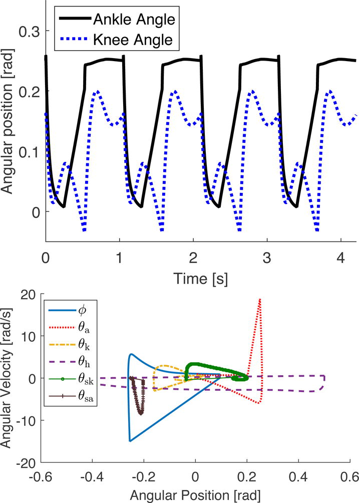
Knee and ankle trajectories of one leg over four steady-state strides of the nominal “human” gait (top), and phase portrait of the biped during one steady step (bottom). This figure is reproduced from [36].

Phase Portraits and Gait Characteristics

Here, we show simulation results with three different shaping strategies. To do this, we plugged in (43) and (44) into (11) to obtain the control law for our simulation. Then, we set μ = 1 so that Ñ = N and progressively changed κ to study the effects of kinetic energy shaping on the biped. Then, we fixed κ = 1 and altered μ to see the independent effects of potential energy shaping. Finally, we increased or decreased both terms concurrently to observe the effects of total energy shaping. For each specific combination of κ and μ, we allowed the biped to converge to a steady gait before recording data. For notational purposes, 0 ≤ κ < 1 indicates we are providing (1 − κ) · 100% support for compensating limb inertia, whereas κ > 1 indicates we are adding (κ − 1) · 100% virtual limb inertia in closed loop. Analogously, 0 < μ < 1 indicates the exoskeleton is providing (1 − μ) · 100% BWS $\left(\stackrel{\sim }{g}<g\right)$, while μ > 1 indicates the exoskeleton is providing (μ − 1) · 100% negative BWS $\left(\stackrel{\sim }{g}>g\right)$.

For a joint-level perspective, Figure 14 compares the phase portraits of the passive gait and the shaped gaits with different shaping strategies. Wider orbits for all joints correspond to longer steps and taller orbits for all joints correspond to faster steps. For the case of kinetic energy shaping (left column), maximum limb inertia compensation (κ = 0) provides greater range of motion and faster joint velocities. The opposite effect is observed for most joints (except the hip) when virtually adding limb inertia (κ = 1.2). The potential energy shaping case (center column) provides the opposite trend: positive BWS (0 < μ < 1) contracts the phase portraits whereas negative BWS (μ > 1) expands them. This verifies the observation in [36] that decreasing potential energy tends to slow down the biped and constrict its range of motion, which has the benefit of greater swing foot clearance to compensate for drop foot. Decreasing (or increasing) both kinetic and potential energy through total energy shaping (right column) renders even greater differences than the potential shaping case (as found in [37]).

Figure 14.

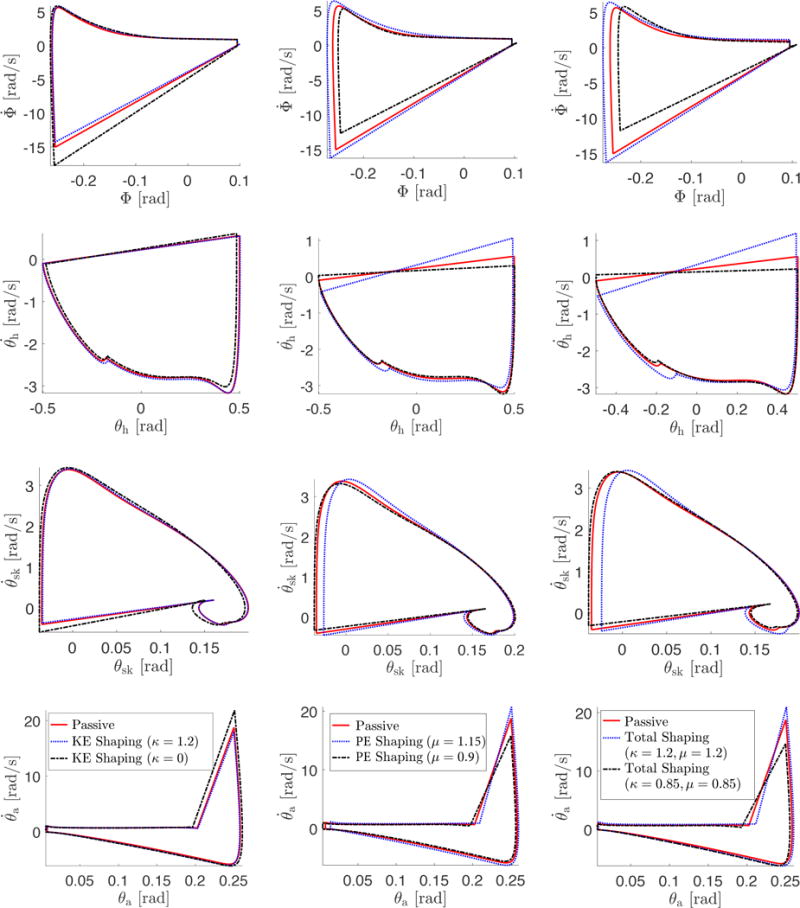
Phase portraits of the passive gait and the shaped gaits. The left column corresponds to the case of kinetic energy shaping, the center column corresponds to the case of potential energy shaping, and the right column corresponds to the case of total energy shaping. Each column shares the same legend shown in the last figure. The rows (from top to bottom) correspond to ϕ, stance hip, swing knee, and stance ankle joints respectively. Each data point on these curves was recorded once steady walking had been achieved.

To further compare the changes in gait characteristics, we show the step length, step linear velocity, and step time periods recorded during simulation with different shaping strategies in Table 3. From this table, we can see that compensating body mass and/or limb inertia in the shapeable dynamics with potential energy shaping and/or total energy shaping decreases the step length as well as the step linear velocity but increases the time periods spent for each step. In contrast, adding virtual body mass and/or limb inertia increases step length and step linear velocity but reduces time interval for each step. Although some of the joint orbits in Figure 14 expanded when compensating limb inertia with kinetic energy shaping only (κ = 0), step length and walking speed decreased because of a contraction in the hip orbit (that is, reduced hip extension causes a shorter step [71]). A similar observation holds for the case of κ = 1.2. These simulation results indicate that different shaping strategies can be chosen based on training goals to promote different gait characteristics.

TABLE 3.

Step length, step linear velocity, and step time periods recorded in simulation with different shaping strategies.

Control strategies	Step length [m]	Step linear velocity [m/s]	Step time periods [s]
Passive (μ = κ = 1)	0.5259	1.0113	0.5256
PE (μ = 1.1)	0.5379	1.1049	0.4868
PE (μ = 1.05)	0.5352	1.0554	0.5071
PE (μ = 0.95)	0.5281	0.9740	0.5421
PE (μ = 0.9)	0.5264	0.9492	0.5546
KE (κ = 2)	0.5677	1.2598	0.4506
KE (κ = 1.2)	0.5368	1.0286	0.5219
KE (κ = 0.8)	0.5259	0.9996	0.5261
KE (κ = 0)	0.5114	0.9807	0.5214
Total (κ = 1.2, μ = 1.2)	0.5424	1.2044	0.4504
Total (κ = 0.85, μ = 0.85)	0.5197	0.9335	0.5567

Metabolic Cost

A key metric for evaluating an exoskeleton is whether it reduces the human user’s metabolic cost of walking [72]. The integral of electromyography (EMG) squared readings from the Soleus and Vastus Lateralis muscles are a good representation of total metabolic cost [73]. Assuming EMG activation is directly related to joint torque production, the authors of [74] proposed a simulation-based metric for metabolic cost

$${\alpha }_j^2=\frac{{\displaystyle {\int }_0^T{v}_j^2\left(t\right)\mathrm{d}t}}{T{\left(\mathit{mgl}\right)}^2}\approx \frac{{\displaystyle {\sum }_{i=1}^{N_T}{v}_j^2\left(i\right)\mathrm{\Delta }t}}{T{\left(\mathit{mgl}\right)}^2},$$ (47)

where T is the step time period, N_T is the number of timesteps in the simulation, v_j is the joint moment, m is the overall mass of the biped, and l is the length of the biped leg. Therefore, we computed the sum of all human joint costs (47) to estimate the effects of energy shaping on the metabolic cost of walking, where several different conditions are shown in Figure 15.

Figure 15.

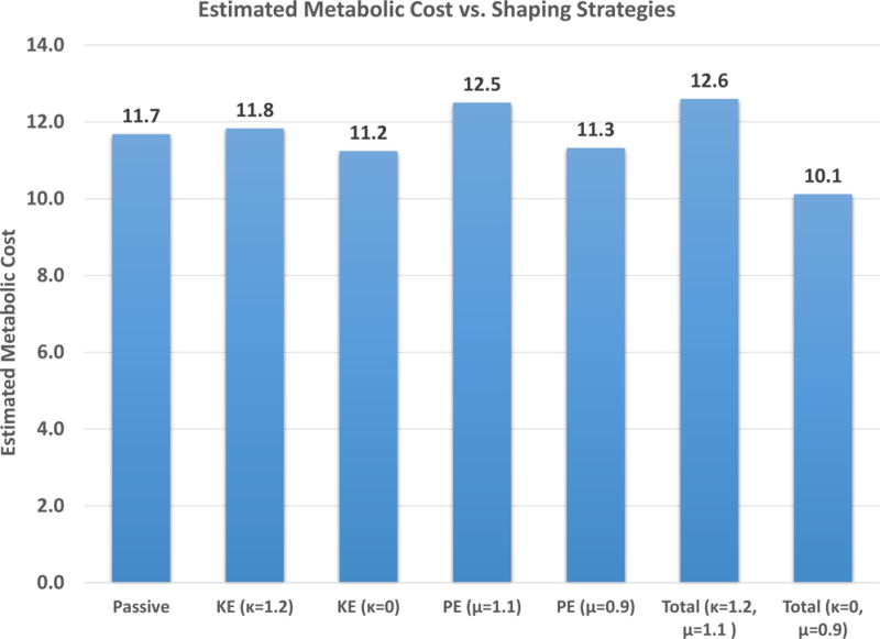
The estimated metabolic costs with different shaping strategies. The numbers on top of each bar denote the sum of (47) for all actuated human joints given the shaping strategy indicated on the x-axis.

From this figure, we can see that adding 20% virtual limb inertia (KE, κ = 1.2) has minor effects on the metabolic cost compared to the passive gait, whereas compensating all the limb inertia (KE, κ = 0) reduces the metabolic cost. Similarly for the case of potential energy shaping, negative BWS (PE, μ = 1.1) increases the biped’s metabolic cost, whereas positive BWS (PE, μ = 0.9) reduces the overall metabolic cost compared to the passive gait. This meets our expectation that offloading the weight of a patient makes it easier to practice walking. For total energy shaping, κ = 1.2 and μ = 1.1 made the biped consume more metabolic energy than only shaping kinetic energy with κ = 1.2 or potential energy with μ = 1.1. When compensating limb inertia in addition to gravity by total energy shaping (κ = 0, μ = 0.9), the biped consumed the least amount of energy compared to all the other cases in Figure 15. These results suggest that the energy shaping approach could provide meaningful assistance during gait rehabilitation, where a clinician can adjust the scaling factors to actively manipulate human effort.

Froude Number

Froude number quantifies the optimal exchange between kinetic and potential energy during dynamic locomotion [75] and has been used to predict the effect of different gravity constants on walking gaits [76]. Two “geometrically similar” bodies that make use of the exchange between kinetic and potential energy to move (for example, pendular motion) will behave in a “dynamically similar” manner if they are associated with the same Froude’s number F_r = ṡ²/gl, where ṡ is the velocity of progression [75], l is leg length, and g is the gravity constant. Assuming F_r remains constant, the effect of gravity on walking speed was predicted by $\dot{\stackrel{\sim }{s}}=\dot{s}\sqrt{\left(\stackrel{\sim }{g}/g\right)}$ in [76]. Therefore, varying gravity $\stackrel{\sim }{g}$ will affect the optimal walking speed $\dot{\stackrel{\sim }{s}}$ such that increased gravity will result in higher velocity and vice versa [77]. To determine whether our simulation results were in agreement with this trend, we calculated predicted velocities $\dot{\stackrel{\sim }{s}}$ with different values of $\stackrel{\sim }{g}$, where $\dot{\stackrel{\sim }{s}}$ was taken as the velocity at μ = 1 (passive gait). Our results in Table 4 show that the trend predicted by Froude number was maintained in the simulation.

TABLE 4.

Analysis of Froude number. The first column contains different values of μ used in the simulation. The second column contains the step linear velocities observed in simulations with the corresponding μ, where each data point was recorded once steady walking had been achieved. The third column contains the predicted linear velocities $\dot{\stackrel{\sim }{s}}$ calculated by multiplying the passive gait’s velocity $\dot{s}=1.011\text{m/s}$ with $\sqrt{\mu }=\sqrt{\stackrel{\sim }{g}/9.81}$.

Control strategies	Step velocity [m/s]	Predicted velocity $\dot{\stackrel{\sim }{s}}$ [m/s]
PE (μ = 0.9)	0.949	0.959
PE (μ = 0.95)	0.974	0.985
Passive (μ = 1)	1.011	1.011
PE (μ = 1.05)	1.055	1.036
PE (μ = 1.1)	1.105	1.060

Human Subject Experiments with Powered Knee-Ankle Exoskeleton

Having demonstrated simulation results on a human-like biped, we wish to implement the energy-shaping control approach on the powered knee-ankle exoskeleton to validate the proposed design and control philosophy. This unilateral device was designed to assist individuals post stroke, who usually have impairments on one side of their body such as diminished leg muscle strength or the inability to generate voluntary muscle contractions with normative magnitude [78]. In this section, we first verify that the device is sufficiently backdrivable during the dynamic conditions of locomotion. Then, we implement a potential energy shaping controller to provide BWS and demonstrate experimental results with an able-bodied subject performing three different activities of daily living. The human subject experiments followed a protocol approved by the Institutional Review Board of the University of Texas at Dallas. During these experiments the subject had the ability to deactivate the exoskeleton by releasing a hand-held safety switch.

Dynamic Backdrive Torque Test

During dynamic conditions backdrive torques must be large enough to overcome the reflected inertia and reflected damping of the actuator, which scale with the gear ratio squared [18]. The low-ratio actuator design of the powered knee-ankle exoskeleton aimed to minimize the reflected inertia and damping for improved dynamic backdrivability. We studied this by monitoring the reaction torque sensors inline with the actuators during dynamic walking conditions with the command torque of both joints set to zero. An able-bodied human subject began this test with active torque compensation enabled, that is, using the outer torque loop in Figure 8. After several steps, the user released the safety button to deactivate the actuator and walked without active torque compensation.

The absolute backdrive torques (averaged over 10 steps) with and without compensation are shown in Figure 16. We see that the peak dynamic backdrive torque is less than 8 Nm at the knee and 5 Nm at the ankle during uncompensated fast walking (1.207 m/s). The peak for the knee occurs at the start of swing phase, where accelerations are highest. The peak for the ankle occurs at initial stance primarily due to acceleration associated with the heel striking the ground. The knee torque is higher than the ankle because of the knee’s higher acceleration. With closed-loop torque control, the peak backdrive torque drops to less than 3 Nm. The mean value of the absolute torque is reduced by 22.9% for the ankle and 63.13% for the knee. The peak backdrive torque is reduced by 57.87% for the ankle and 63.56% for the knee [34]. These backdrive torques are an order of magnitude smaller than normative human joint torques [44] and would likely be even smaller in a clinical application, where slower walking speeds are expected. Improved alignment of the exoskeleton brace with the anatomical joint axes of rotation could further reduce the backdrive torques.

Figure 16.

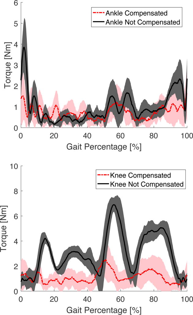
Measured backdrive torque during passive walking: average absolute values and error bars (±1 standard deviation shown in shaded regions) of 10 steady steps. This figure is reproduced from [34].

Underactuated Potential Energy Shaping for a Unilateral Exoskeleton

Gait rehabilitation after a stroke often involves locomotor training while a fraction of the patient’s body weight is offloaded by a harness [79]. This inspires us to implement potential energy shaping on the unilateral powered knee-ankle exoskeleton to provide BWS on the affected side. This part reports the implementation and preliminary experiments with an able-bodied human subject.

Controller Implementation

To implement the potential energy shaping controller, we first set $M_{\lambda }={\stackrel{\sim }{M}}_{\lambda }$ in (42), that is, not shaping the kinetic energy. Because we are interested in controlling a unilateral knee-ankle exoskeleton using only feedback local to its leg, we separate the dynamical models of the stance and swing legs for the purpose of control derivation. The configuration vectors for both the stance and swing models are given as

$$q_{\text{st}}={\left(p_{\mathrm{x}},p_{\mathrm{y}},\varphi ,{\theta }_{\mathrm{a}},{\theta }_{\mathrm{k}}\right)}^T\in {\mathrm{ℝ}}^5,q_{\text{sw}}={\left(h_{\mathrm{x}},h_{\mathrm{y}},{\theta }_{\text{th}},{\theta }_{\text{sk}},{\theta }_{\text{sa}}\right)}^T\in {\mathrm{ℝ}}^5.$$

The subscripts “st” and “sw” indicate stance and swing, and the stance leg configuration q_st is defined similar to the full biped model configuration vector q. We choose the hip as a floating base for the swing leg’s kinematic chain, where (h_x, h_y)^T are the Cartesian positions of the hip, and θ_th is the absolute angle from the vertical axis to the swing thigh. Derivations in [36] demonstrate that the proposed matching framework yields a uniform stance control law u_st (equivalent across stance contact conditions) and swing control law u_sw as

$$u_{\text{st}}=\left(1-\mu \right)N_{\text{st}\left(4,5\right)},u_{\text{sw}}=\left(1-\mu \right)N_{\text{sw}\left(4,5\right)}.$$ (48)

These control laws only require position feedback, where joint angles are measured by joint encoders and global orientation is measured by the IMU. Moreover, the control laws do not prescribe joint kinematics and thus are able to provide task-invariant assistance. Instead of recognizing the user’s intention to switch between numerous controllers in a finite-state machine [13], [80]–[82], the control law (48) switches only between stance and swing. The model parameters used in these two control laws are given in Table 5. The following experiments with potential energy shaping did not utilize the outer torque loop in Figure 8 because the previously reported dynamic backdrive torques were acceptably small without active torque compensation (and it would be desirable to remove expensive torque sensors in future designs).

TABLE 5.

Model parameters for the potential energy shaping controller implemented on the knee-ankle exoskeleton for human subject experiments. The segment masses of the subject were calculated based on [44]. The lengths of the subject’s limbs and the exoskeleton masses were measured. The exoskeleton and human masses were combined in the control law calculation to provide weight support for both the human and exoskeleton.

Parameter	Variable	Value
Hip and upper body mass	mh	54.835 [kg]
Thigh mass	mt	11.228 [kg]
Shank mass	ms	6.582 [kg]
Foot mass	mf	1.745 [kg]
Knee exoskeleton mass	mk	2.106 [kg]
Ankle exoskeleton mass	ma	1.843 [kg]
Shoe insert mass	msh	0.356 [kg]
Shank length	ls	0.41 [m]
Thigh length	lt	0.44 [m]
Foot length	lf	0.2736 [m]

Treadmill Walking Test

The first experimental task with potential energy shaping was walking on a treadmill (Figure 17, top left). A safety harness was used to prevent potential falls. Before recording data, the subject was given time to acclimate to the unpowered exoskeleton and find a natural walking gait. Then the subject was asked to stand straight while the exoskeleton’s sensors were initialized. After activating the controller with positive or negative BWS, the subject started walking on the treadmill at a constant speed of 0.894 m/s. Data was recorded for twelve strides after the subject achieved a steady gait.

Figure 17.

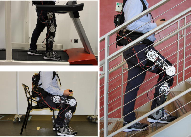
Photos of multiple task experiments. Top left: treadmill test, bottom left: sit-to-stand-to-sit test, right: stair ascent/descent tests.

During the positive BWS walking test, the exoskeleton applied 10% BWS during stance and 20% BWS during swing. A larger BWS ratio was used during the swing phase to increase the torque amplitude. Figures 18(a)–18(b) show the commanded and measured torques (averaged over 12 strides) in comparison to the normative human joint torques [44] scaled by the BWS ratio. The ankle actuator generated positive (dorsiflexion) torque during early stance and negative (plantarflexion) torque during late stance to help the subject with weight acceptance and push off, respectively. The knee actuator generated positive (extension) torque during most of stance to offload body weight from the subject’s knee joint. The subject reported feeling assistance and was able to walk comfortably.

Figure 18.

Measured torque from walking tests (averaged over 12 strides). For the knee torque, positive indicates extension while negative indicates flexion. For the ankle torque, positive indicates dorsiflexion while negative indicates plantarflexion. For positive BWS walking test, we set the BWS ratio to be (BWS_st, BWS_sw) = (10%, 20%), whereas the negative BWS walking test had (BWS_st, BWS_sw) = (−5%, −10%). Winter’s able-bodied torque is obtained by multiplying the normalized torque data from [44] with the subject mass and BWS ratio.

The second test added virtual weight to the subject with −5% BWS during stance and −10% BWS during swing. The resulting torques are shown in Figures 18(c) and 18(d). Instead of assisting the subject, both the knee and ankle actuators generated flexion torques during stance to prevent the subject from extending his joints. The subject reported having to expend more effort to continue walking at 0.894 m/s under the added virtual weight. In this test the signs of the actuator torques tended to be the opposite of the able-bodied references (providing resistance), whereas the signs tended to be aligned during the positive BWS test (providing assistance). In both cases, the torque outputs tracked the reference torques reasonably well during the stance period but not as well during the faster motions of the swing period, where the actuator’s reflected inertia has more influence. This could be addressed in the future by utilizing the outer torque loop or further reducing the transmission ratio, as discussed later.

Sit-to-Stand-to-Sit Test

To study the effects of the energy shaping controller during sit-stand transitions, we asked the subject to stand up from a sitting posture and then immediately sit back down (Figure 17, bottom left). This cycle was repeated 5 times with a 1 to 2 second break each time. The safety harness could not be used in the sitting posture, so we set the BWS ratio to 5% and did not attempt negative BWS in order to minimize the risk of falling. Figures 19(a) and 19(b) shows that both the knee and ankle actuators provided extension torques to offload the user’s body weight while standing up and sitting down. As a consequence, the standing motion was accelerated while the sitting motion was slowed, so the standing motion accounts for only 35% of the cycle. The subject reported feeling that the sit-to-stand cycle was easier with the assistance.

Figure 19.

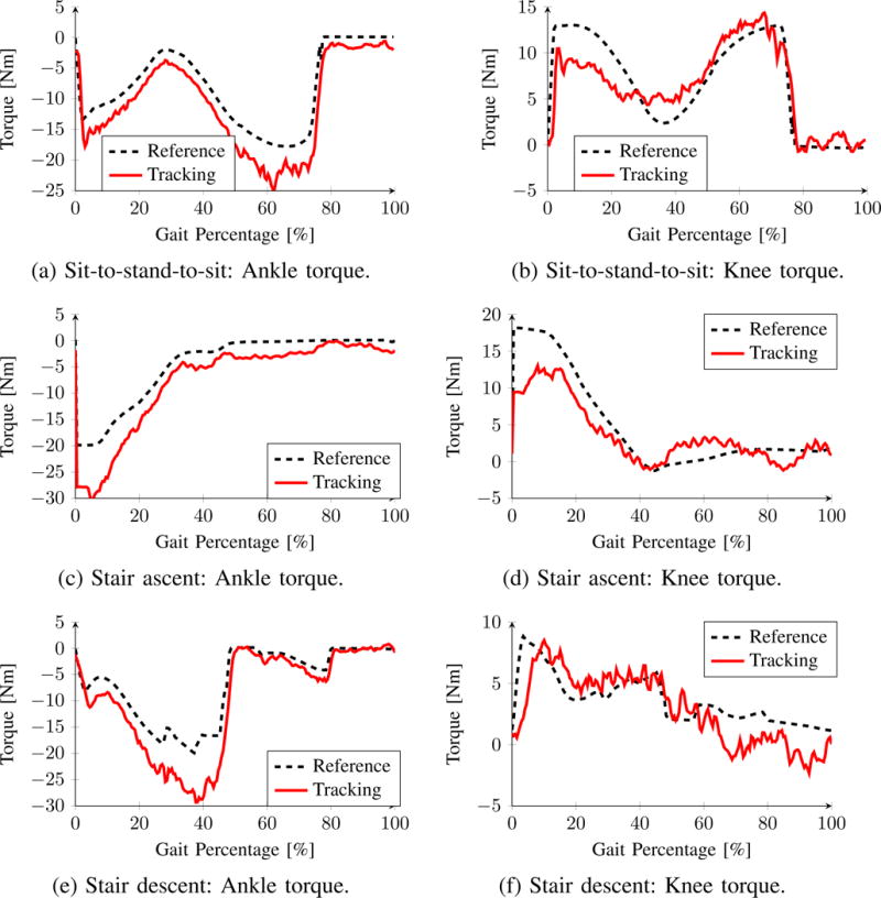
Measured torque from the sit-to-stand-to-sit test (averaged over 5 cycles) and the stair ascent/descent tests (each averaged over 7 strides). The direction of torques align with the ones in Figures 18(a) to 18(d). For the sit-to-stand-to-sit test we set the BWS ratio to 5%. For both stair ascent and descent tests, we set the BWS ratio to 10% for both the stance and swing controllers.

Stair Climbing Test

The stair climbing test (Figure 17, right) was performed on an indoor staircase with handrails. We began data recording from the first step until the subject reached the end of the stairs (a total of 7 steps). Once the subject finished climbing, we asked him to turn around and walk downstairs. For safety reasons, we only provided the subject with 10% BWS going up and down the stairs, and negative BWS was not attempted. The recorded data for upstairs and downstairs are shown in Figures 19(c) to 19(f). The ankle actuator provided plantarflexion torque and the knee actuator provided extension torque during stance to offload body weight, reducing the user’s effort to propel their COM up the stairs or decelerate their COM during stair descent. The subject was able to walk stably and reported feeling comfortable and confident during both locomotor tasks without holding the handrail.

Limitations and Future Research

Although these simulation and experimental results demonstrate the potential of the proposed design and control philosophy, some limitations still remain to be overcome. First and foremost, kinetic energy shaping needs to be implemented in hardware. The control law (42) depends on M_λ and ${\stackrel{\sim }{M}}_{\lambda }$, which include mass/inertia parameters of the exoskeleton and human limbs. The exoskeleton parameters can be estimated using standard system identification methods [5], and human parameters can be estimated from the user’s weight and limb lengths based on formulas from cadaver studies [70]. Parametric errors will result in slightly different closed-loop system parameters than anticipated, but the overall effect of inertia and/or weight compensation will still be achieved. In other words, the actuator torques will still provide assistance/resistance but will be in different magnitudes due to parameter uncertainties.

Future work for control design includes shaping not only the limb inertias but also the mass terms in the inertia matrix. The main challenge is to ensure the positive definiteness of the shaped mass/inertia matrix so the control law remains well-defined. Future work could also attempt to avoid the algebraic simplifications used to solve the matching conditions (that is, shaping only the actuated coordinates), which could provide more effective shaping strategies for human assistance. Ultimately, we will investigate how the choice of $\stackrel{\sim }{M}$ promotes different gait characteristics in both able-bodied human subjects and individuals post stroke.

Although the powered knee-ankle exoskeleton provided adequate backdrivability and torque density, significant improvements can still be made. It would be desirable to further reduce the dynamic backdrive torque and improve torque tracking (without a torque sensor) through the use of an even lower transmission ratio. The presented prototype is also cumbersome to don and doff for the user. Therefore, ongoing work includes the design and testing of our next-generation powered knee orthosis (Generation Two, Figure 1(c)). This device has a custom PMSM motor with greater torque density to allow the use of a 7:1 one-stage planetary gearbox, which has about 1/10 the reflected inertia of the Generation One actuator. This design aims to assist elderly individuals and enhance the capabilities of fully able-bodied users, and it will be tested in both unilateral and bilateral configurations depending on user needs.

Conclusion

In this paper, we summarized our past and ongoing work to present our design and control philosophy for highly-backdrivable lower-limb exoskeletons. By combining torque-dense electrical motors and low-ratio custom transmissions, high torque output and intrinsic backdrivability were achieved simultaneously with minimal production cost. To provide human-cooperative exoskeletal assistance, we proposed a complete theoretical framework for underactuated total energy shaping that incorporates both environmental and human interaction. This general matching framework yields task-invariant, trajectory-free control laws that can accommodate different activities of daily living. Next, we simulated different energy shaping strategies on a human-like 8-DOF biped to study their possible effects and benefits for human assistance. Finally, we implemented the potential energy shaping strategy on the designed knee-ankle exoskeleton and conducted experiments with an able-bodied subject. The subject was free to move his joints with minimal resistance from the exoskeleton actuators, and the potential energy shaping controller provided the subject with consistent assistance during positive BWS tests or resistance during negative BWS tests. Future work will further refine this design/control philosophy and study clinical outcomes for different patient populations.

Sidebar: Summary of the Paper

The majority of assistive exoskeletons are designed to rigidly track time-based kinematic patterns using highly geared actuators, which prevents users from moving their joints freely without help from the exoskeleton. Individuals with partial or full volitional control of their lower extremities require novel design and control methods for exoskeletons that are more compatible with human interaction. In order to assist or augment volitional human motion, exoskeleton joints must be backdrivable and the control strategy must be invariant to the user’s joint kinematics. This paper presents the design philosophy behind two generations of highly backdrivable exoskeletons, which utilize torque-dense motors with low-ratio transmissions. To leverage these designs, a torque-based control framework is presented that shapes the human body’s kinetic and potential energies to provide trajectory-free assistance. Simulations with a human-like biped demonstrate the effects of different energy shaping control strategies, and experiments with a powered knee-ankle exoskeleton demonstrate the user-cooperative and task-invariant nature of the control approach. These results demonstrate potential value for gait assistance and augmentation without being constrained to a clinical environment like traditional treadmill training devices. To achieve the control design and implementation, one would need knowledge of linear algebra, robot dynamics, state-space control, and LabVIEW programming.

Sidebar: Passivity and Stability Properties

Consider a n-link robot described by the following equations of motion

$$M\left(q\right)\ddot{q}+C\left(q,\dot{q}\right)\dot{q}+N\left(q\right)=\tau ,$$ (S1)

where q ∈ ℝⁿ is the configuration vector, and $\dot{q}\in {\mathrm{ℝ}}^n$ is the velocity vector. The positive-definite matrix M(q) ∈ ℝ^n×n is the mass/inertia matrix, $C\left(q,\dot{q}\right)\in {\mathrm{ℝ}}^{n\times n}$ is the Coriolis/centrifugal matrix, N(q) ∈ ℝⁿ is the gravitational forces vector defined as the gradient of the robot’s potential energy, and τ ∈ ℝⁿ is the torque input vector.

Let S(x) : ℝⁿ → ℝ be a continuously differentiable non-negative scalar function, then the system (S1) is said to be passive from input τ to output y with storage function S(x) if $\dot{S}\left(x\right)\le y^T\tau$. Passivity indicates that the change in the robot’s energy is bounded by the “energy” injected through the input τ. In other words, the robot cannot generate “energy” on its own. For robots with dynamics of the form (S1), input-output passivity can be shown by choosing $y={\dot{q}}^T$ and the robot’s total energy $H\left(q,\dot{q}\right)$ as the storage function:

$$H\left(q,\dot{q}\right)=\frac{1}{2}{\dot{q}}^{T}M\left(q\right)\dot{q}+P\left(q\right).$$ (S2)

Taking the time derivative of $H\left(q,\dot{q}\right)$ yields

$$\begin{gathered} \dot{H}={\dot{q}}^{T}M\left(q\right)\ddot{q}+\frac{1}{2}{\dot{q}}^T\dot{M}\left(q\right)\dot{q}+{\dot{q}}^{T}N\left(q\right) \\ ={\dot{q}}^T\left(\tau -C\left(q,\dot{q}\right)\dot{q}-N\left(q\right)\right)+\frac{1}{2}{\dot{q}}^T\dot{M}\left(q\right)\dot{q}+{\dot{q}}^{T}N\left(q\right), \end{gathered}$$

where $M\left(q\right)\ddot{q}$ has been substituted using the equations of motion (S1). Canceling out ${\dot{q}}^{T}N\left(q\right)$ and collecting terms yields

$$\begin{gathered} \dot{H}={\dot{q}}^T\tau +\frac{1}{2}{\dot{q}}^T\left(\dot{M}\left(q\right)-2C\left(q,\dot{q}\right)\right)\dot{q} \\ ={\dot{q}}^T\tau , \end{gathered}$$ (S3)

where the second equality holds true based on the skew-symmetry property between M(q) and $C\left(q,\dot{q}\right)$, that is, $\dot{M}\left(q\right)-2C\left(q,\dot{q}\right)=-{\left(\dot{M}\left(q\right)-2C\left(q,\dot{q}\right)\right)}^T$ [S1].

Input-output passivity enables several stability results through passivity-based control. For example, negative feedback of the output through the input guarantees asymptotic convergence of the output to zero [S1]. We first leverage a standard result for passive systems to state the following [S2]:

Proposition 1

Consider the passive system (S1) with input τ and output $y=\dot{q}$. Given output feedback control τ = σ(y), where σ is any continuous function satisfying y^Tσ(y) ≤ 0, then lim_t→∞ y(t) → 0 and the origin $\left(q,\dot{q}\right)=\left(0,0\right)$ is stable in the sense of Lyapunov.

Here we highlight one possible stability result from [S3] for the case of potential energy shaping. In [S3] we proved that potential energy shaping preserves the passive mapping from the human input τ_hum to output $y={\dot{q}}^T$ in closed loop. This proof relies on the closed-loop total energy $\stackrel{\sim }{H}$ as the storage function:

$$\stackrel{\sim }{H}\left(q,\dot{q}\right)=\frac{1}{2}{\dot{q}}^{T}M\left(q\right)\dot{q}+\stackrel{\sim }{P}\left(q\right),$$ (S4)

where $\stackrel{\sim }{P}\left(q\right):={\displaystyle {\int }_0^q{\displaystyle {\sum }_{i=1}^n{\stackrel{\sim }{N}}_{\left(i\right)}\left(s\right)}}$ ds is the closed-loop potential energy.

It is well established that human motor control effectively modulates joint impedance, that is, the stiffness and viscosity of a joint [S5], [S6]. Therefore, in [S3] we assume the human input takes the form of an impedance controller (which we used for our simulations in this paper) given by τ_hum = −K_pe − K_dė, where K_p and K_d are two positive-definite diagonal matrices, $e:=q-\overline{q}$ is the difference between q and the fixed equilibria vector $\overline{q}$, and $\dot{e}=\dot{q}=y$. To utilize Lyapunov stability analysis, we define a Lyapunov function

$$V\left(q,\dot{q}\right)=\stackrel{\sim }{H}\left(q,\dot{q}\right)+\frac{1}{2}{e}^T{K}_{\mathrm{p}}e.$$ (S5)

It is clear that adding a quadratic term $\frac{1}{2}{e}^T{K}_{\mathrm{p}}e$ to the positive-definite $\stackrel{\sim }{H}\left(q,\dot{q}\right)$ produces a positive-definite function. Taking the time derivative of $V\left(q,\dot{q}\right)$ yields

$$\begin{gathered} \dot{V}\left(q,\dot{q}\right)=y^T{\tau }_{\text{hum}}+{\dot{e}}^T{K}_{\mathrm{p}}e \\ =y^T\left(-K_{\mathrm{p}}e-K_{\mathrm{d}}\dot{e}+K_{\mathrm{p}}e\right) \\ =-y^T{K}_{\mathrm{d}}y\le 0, \end{gathered}$$ (S6)

implying that the shaped human leg is Lyapunov stable [S4].

Biographies

Ge Lv received the B.S. (2011) and the M.S. (2013) degrees in information science and engineering from Northeastern University, Shenyang, China. He joined the Department of Electrical Engineering at the University of Texas at Dallas (UTD) as a Ph.D. student in 2013. His research is in the control of bipedal locomotion with applications to orthoses and exoskeletons. He received the Best Student Paper Award of the 2015 IEEE Conference on Decision and Control.

Hanqi Zhu received the B.S. (2011) and the M.S. (2013) degrees in mechanical engineering from the Xi’an Jiaotong University, China. He is pursuing a second M.S. degree and a Ph.D. degree in the Department of Electrical Engineering at UTD. His research is in the design of advanced mechatronics systems with applications to wearable rehabilitation robots.

Robert D. Gregg received the B.S. degree (2006) in electrical engineering and computer sciences from the University of California, Berkeley and the M.S. (2007) and Ph.D. (2010) degrees in electrical and computer engineering from the University of Illinois at Urbana-Champaign. He joined the Departments of Bioengineering and Mechanical Engineering at UTD as an Assistant Professor in 2013. Prior to joining UTD, he was a Research Scientist at the Rehabilitation Institute of Chicago and a Postdoctoral Fellow at Northwestern University. His research is in the control of bipedal locomotion with applications to autonomous and wearable robots. He is a Senior Member of the IEEE.

References

- S1.Spong M, Hutchinson S, Vidyasagar M. Robot Modeling and Control. Vol. 3 Wiley; New York: 2006. [Google Scholar]
- S2.Sepulchre R, Jankovic M, Kokotovic PV. Constructive Nonlinear Control. Springer; 2012. [Google Scholar]
- S3.Lv G, Gregg RD. Underactuated potential energy shaping with contact constraints: Application to a powered knee-ankle orthosis. IEEE Trans Control Syst Technol. 2018 Jan;26(1):181–193. doi: 10.1109/TCST.2016.2646319. [DOI] [PMC free article] [PubMed] [Google Scholar]
- S4.Murray RM, Li Z, Sastry SS. A Mathematical Introduction to Robotic Manipulation. Boca Raton, FL, USA: CRC Press; 1994. [Google Scholar]
- S5.Flash T, Hogan N. The coordination of arm movements: An experimentally confirmed mathematical model. J Neurosci. 1985 Jul;5(7):1688–1703. doi: 10.1523/JNEUROSCI.05-07-01688.1985. [DOI] [PMC free article] [PubMed] [Google Scholar]
- S6.Burdet E, Osu R, Franklin DW, Milner TE, Kawato M. The central nervous system stabilizes unstable dynamics by learning optimal impedance. Nature. 2001;414(6862):446–449. doi: 10.1038/35106566. [DOI] [PubMed] [Google Scholar]
Acknowledgments
This work was supported by the National Institute of Child Health & Human Development of the NIH under Award Number DP2HD080349. This work was also supported by NSF Award CMMI-1652514. The content is solely the responsibility of the authors and does not necessarily represent the official views of the NIH or the NSF. R. D. Gregg holds a Career Award at the Scientific Interface from the Burroughs Wellcome Fund.
- 1.Yan T, Cempini M, Oddo CM, Vitiello N. Review of assistive strategies in powered lower-limb orthoses and exoskeletons. Rob Auton Syst. 2015;64:120–136. [Google Scholar]
- 2.Zeilig G, Weingarden H, Zwecker M, Dudkiewicz I, Bloch A, Esquenazi A. Safety and tolerance of the rewalk exoskeleton suit for ambulation by people with complete spinal cord injury: A pilot study. The Journal of Spinal Cord Medicine. 2012;35(2):96–101. doi: 10.1179/2045772312Y.0000000003. [DOI] [PMC free article] [PubMed] [Google Scholar]
- 3.Kolakowsky-Hayner SA, Crew J, Moran S, Shah A. Safety and feasibility of using the Ekso Binoic exoskeleton to aid ambulation after spinal cord injury. J Spine. 2013;4:003. [Google Scholar]
- 4.Agrawal A, Harib O, Hereid A, Finet S, Masselin M, Praly L, Ames AD, Sreenath K, Grizzle JW. First steps towards translating hzd control of bipedal robots to decentralized control of exoskeletons. IEEE Access. 2017;5:9919–9934. [Google Scholar]
- 5.Ghan J, Steger R, Kazerooni H. Control and system identification for the Berkeley Lower Extremity Exoskeleton (BLEEX) Adv Rob. 2006;20(9):989–1014. [Google Scholar]
- 6.Quinlivan B, Lee S, Malcolm P, Rossi D, Grimmer M, Siviy C, Karavas N, Wagner D, Asbeck A, Galiana I, et al. Assistance magnitude versus metabolic cost reductions for a tethered multiarticular soft exosuit. Science Robotics. 2017;2(2):4416–4416. doi: 10.1126/scirobotics.aah4416. [DOI] [PubMed] [Google Scholar]
- 7.Pratt JE, Krupp BT, Morse CJ, Collins SH. IEEE Int Conf Robot Autom. Vol. 3. IEEE; 2004. The roboknee: An exoskeleton for enhancing strength and endurance during walking; pp. 2430–2435. [Google Scholar]
- 8.Blaya JA, Herr H. Adaptive control of a variable-impedance ankle-foot orthosis to assist drop-foot gait. IEEE Trans Neural Syst Rehabil Eng. 2004;12(1):24–31. doi: 10.1109/TNSRE.2003.823266. [DOI] [PubMed] [Google Scholar]
- 9.Kawamoto H, Sankai Y. Power assist system HAL-3 for gait disorder person. Computers helping people with special needs. 2002:196–203. [Google Scholar]
- 10.Aguilar-Sierra H, Lopez R, Yu W, Salazar S, Lozano R. A lower limb exoskeleton with hybrid actuation. IEEE Int Conf Biomedical Robotics and Biomechatronics IEEE. 2014:695–700. [Google Scholar]
- 11.Lu R, Li Z, Su C-Y, Xue A. Development and learning control of a human limb with a rehabilitation exoskeleton. IEEE Trans Ind Electron. 2014;61(7):3776–3785. [Google Scholar]
- 12.Kiguchi K, Yokomine Y. Walking assist for a stroke survivor with a power-assist exoskeleton. IEEE Int Conf Systems, Man and Cybernetics IEEE. 2014:1888–1892. [Google Scholar]
- 13.Murray SA, Ha KH, Hartigan C, Goldfarb M. An assistive control approach for a lower-limb exoskeleton to facilitate recovery of walking following stroke. IEEE Trans Neural Syst Rehabil Eng. 2015;23(3):441–449. doi: 10.1109/TNSRE.2014.2346193. [DOI] [PubMed] [Google Scholar]
- 14.Jimenez-Fabian R, Verlinden O. Review of control algorithms for robotic ankle systems in lower-limb orthoses, prostheses, and exoskeletons. Medical Engineering & Physics. 2012;34(4):397–408. doi: 10.1016/j.medengphy.2011.11.018. [DOI] [PubMed] [Google Scholar]
- 15.Gregg RD, Lenzi T, Hargrove LJ, Sensinger JW. Virtual constraint control of a powered prosthetic leg: From simulation to experiments with transfemoral amputees. IEEE Trans Rob. 2014 Dec;30(6):1455–1471. doi: 10.1109/TRO.2014.2361937. [DOI] [PMC free article] [PubMed] [Google Scholar]
- 16.Quintero D, Villarreal DJ, Lambert DJ, Kapp S, Gregg RD. Continuous-phase control of a powered knee–ankle prosthesis: Amputee experiments across speeds and inclines. IEEE Trans Rob. 2018 doi: 10.1109/TRO.2018.2794536. [DOI] [PMC free article] [PubMed] [Google Scholar]
- 17.Duschau-Wicke A, Brunsch T, Lunenburger L, Riener R. Intelligent Robots and Systems, 2008 IEEE/RSJ International Conference on. IEEE; 2008. Adaptive support for patient-cooperative gait rehabilitation with the Lokomat; pp. 2357–2361. [Google Scholar]
- 18.Seok S, Wang A, Chuah MYM, Hyun DJ, Lee J, Otten DM, Lang JH, Kim S. Design principles for energy-efficient legged locomotion and implementation on the MIT Cheetah robot. IEEE/ASME Trans Mechatron. 2015;20(3):1117–1129. [Google Scholar]
- 19.Park H-W, Wensing PM, Kim S. High-speed bounding with the MIT Cheetah 2: Control design and experiments. Int J Rob Res. 2017;36(2):167–192. [Google Scholar]
- 20.Ferris R, Quintero H, Goldfarb M. Preliminary evaluation of a powered lower limb orthosis to aid walking in paraplegic individuals. IEEE Trans Neural Syst Rehabil Eng. 2011;19(6):652–659. doi: 10.1109/TNSRE.2011.2163083. [DOI] [PMC free article] [PubMed] [Google Scholar]
- 21.Kaminaga H, Amari T, Niwa Y, Nakamura Y. Development of knee power assist using backdrivable electro-hydrostatic actuator. IEEE Int Conf Intelligent Robots & Systems. 2010:5517–5524. [Google Scholar]
- 22.Bhounsule PA, Cortell J, Grewal A, Hendriksen B, Karssen JD, Paul C, Ruina A. Low-bandwidth reflex-based control for lower power walking: 65 km on a single battery charge. Int J Rob Res. 2014;33(10):1305–1321. [Google Scholar]
- 23.Kong K, Bae J, Tomizuka M. Control of rotary series elastic actuator for ideal force-mode actuation in human–robot interaction applications. IEEE/ASME Trans Mechatron. 2009;14(1):105–118. [Google Scholar]
- 24.Kong K, Bae J, Tomizuka M. A compact rotary series elastic actuator for human assistive systems. IEEE/ASME Trans Mechatron. 2012;17(2):288–297. [Google Scholar]
- 25.Yu H, Sta Cruz M, Chen G, Huang S, Zhu C, Chew E, Ng YS, Thakor NV. IEEE Int Conf Robot Autom. IEEE; 2013. Mechanical design of a portable knee-ankle-foot robot; pp. 2183–2188. [Google Scholar]
- 26.Brackx B, Geeroms J, Vantilt J, Grosu V, Junius K, Cuypers H, Vanderborght B, Lefeber D. Design of a modular add-on compliant actuator to convert an orthosis into an assistive exoskeleton. IEEE Int Conf Biomedical Robotics and Biomechatronics IEEE. 2014:485–490. [Google Scholar]
- 27.Robinson DW. Ph D dissertation. Massachusetts Institute of Technology; 2000. Design and analysis of series elasticity in closed-loop actuator force control. [Google Scholar]
- 28.Asbeck AT, De Rossi SM, Holt KG, Walsh CJ. A biologically inspired soft exosuit for walking assistance. Int J Rob Res. 2015;34(6):744–762. [Google Scholar]
- 29.Kenneally G, De A, Koditschek DE. Design principles for a family of direct-drive legged robots. IEEE Rob Autom Lett. 2016;1(2):900–907. [Google Scholar]
- 30.Nagarajan U, Aguirre-Ollinger G, Goswami A. Integral admittance shaping: A unified framework for active exoskeleton control. Rob Auton Syst. 2016;75:310–324. [Google Scholar]
- 31.Aguirre-Ollinger G, Colgate JE, Peshkin MA, Goswami A. Inertia compensation control of a one-degree-of-freedom exoskeleton for lower-limb assistance: Initial experiments. IEEE Trans Neural Syst Rehabil Eng. 2012;20(1):68–77. doi: 10.1109/TNSRE.2011.2176960. [DOI] [PubMed] [Google Scholar]
- 32.Holm JK, Spong MW. Kinetic energy shaping for gait regulation of underactuated bipeds. Proc IEEE Int Conf Control Appl. 2008:1232–1238. [Google Scholar]
- 33.Lv G, Zhu H, Elery T, Li L, Gregg RD. Experimental implementation of underactuated potential energy shaping on a powered ankle-foot orthosis. IEEE Int Conf Robot Autom. 2016:3493–3500. doi: 10.1109/ICRA.2016.7487529. [DOI] [PMC free article] [PubMed] [Google Scholar]
- 34.Zhu H, Doan J, Stence C, Lv G, Elery T, Gregg R. Design and validation of a torque dense, highly backdrivable powered knee-ankle orthosis. IEEE Int Conf Robot Autom. 2017 May;:504–510. doi: 10.1109/ICRA.2017.7989063. [DOI] [PMC free article] [PubMed] [Google Scholar]
- 35.Lv G, Gregg RD. Orthotic body-weight support through underactuated potential energy shaping with contact constraints. Proc IEEE Conf Decis Control. 2015:1483–1490. doi: 10.1109/cdc.2015.7402420. [DOI] [PMC free article] [PubMed] [Google Scholar]
- 36.Lv G, Gregg RD. Underactuated potential energy shaping with contact constraints: Application to a powered knee-ankle orthosis. IEEE Trans Control Syst Technol. 2018;26(1):181–193. doi: 10.1109/TCST.2016.2646319. [DOI] [PMC free article] [PubMed] [Google Scholar]
- 37.Lv G, Gregg RD. Towards total energy shaping control of lower-limb exoskeletons. American Control Conference IEEE. 2017:4851–4857. doi: 10.23919/ACC.2017.7963706. [DOI] [PMC free article] [PubMed] [Google Scholar]
- 38.Elery T, Rezazadeh S, Nesler C, Doan J, Zhu H, Gregg R. Design and benchtop validation of a powered knee-ankle prosthesis with high-torque, low-impedance actuators. IEEE Int Conf Robot Autom. 2018 doi: 10.1109/ICRA.2018.8461259. [DOI] [PMC free article] [PubMed] [Google Scholar]
- 39.Waters RL, Mulroy S. The energy expenditure of normal and pathologic gait. Gait & Posture. 1999;9(3):207–231. doi: 10.1016/s0966-6362(99)00009-0. [DOI] [PubMed] [Google Scholar]
- 40.del Castillo JM. The analytical expression of the efficiency of planetary gear trains. Mechanism and Machine Theory. 2002;37(2):197–214. [Google Scholar]
- 41.Krishnan R. Permanent magnet synchronous and brushless DC motor drives. CRC press; 2009. [Google Scholar]
- 42.Dohring ME, Lee E, Newman WS. A load-dependent transmission friction model: theory and experiments. IEEE Int Conf Robotics & Automation. 1993:430–436. [Google Scholar]
- 43.Sensinger JW. Efficiency of high-sensitivity gear trains, such as cycloid drives. ASME J Mechanical Design. 2013;135(7):071006. [Google Scholar]
- 44.Winter DA. Biomechanics and Motor Control of Human Movement. 2nd. New York, NY: Wiley; 2009. [Google Scholar]
- 45.Young AJ, Ferris DP. State of the art and future directions for lower limb robotic exoskeletons. IEEE Trans Neural Syst Rehabil Eng. 2017;25(2):171–182. doi: 10.1109/TNSRE.2016.2521160. [DOI] [PubMed] [Google Scholar]
- 46.Goswami A, Thuilot B, Espiau B. A study of the passive gait of a compass-like biped robot: Symmetry and chaos. Int J Robot Res. 1998;17(12):1282–1301. [Google Scholar]
- 47.McGeer T, et al. Passive dynamic walking. I J Robotic Res. 1990;9(2):62–82. [Google Scholar]
- 48.Gregg RD, Bred TW, Spong MW. A control theoretic approach to robot-assisted locomotor therapy. Proc IEEE Conf Decis Control. 2010:1679–1686. [Google Scholar]
- 49.Holm JK, Lee D, Spong MW. IEEE Int Conf Robot Autom. IEEE; 2007. Time-scaling trajectories of passive-dynamic bipedal robots; pp. 3603–3608. [Google Scholar]
- 50.Ortega R, Perez JAL, Nicklasson PJ, Sira-Ramirez H. Passivity-Based Control of Euler-Lagrange Systems: Mechanical, Electrical and Electromechanical Applications. Berlin, Germany: Springer Science; 1998. [Google Scholar]
- 51.Ortega R, Van der Schaft AJ, Mareels I, Maschke B. Putting energy back in control. IEEE Control Syst Mag. 2001;21(2):18–33. [Google Scholar]
- 52.Blankenstein G, Ortega R, Van Der Schaft AJ. The matching conditions of controlled Lagrangians and IDA-passivity based control. Int J Control. 2002;75(9):645–665. [Google Scholar]
- 53.Ortega R, Spong MW, Gomez-Estern F, Blankenstein G. Stabilization of a class of underactuated mechanical systems via interconnection and damping assignment. IEEE Trans Automat Contr. 2002;47(8):1218–1233. [Google Scholar]
- 54.Bloch AM, Chang DE, Leonard NE, Marsden JE. Controlled Lagrangians and the stabilization of mechanical systems II: Potential shaping. IEEE Trans Automat Contr. 2001;46(10):1556–1571. [Google Scholar]
- 55.Holm J. Ph D dissertation. University of Illinois at Urbana-Champaign; 2008. Gait regulation for robotic bipedal locomotion. [Google Scholar]
- 56.Murray RM, Li Z, Sastry SS. A Mathematical Introduction to Robotic Manipulation. CRC press; 1994. [Google Scholar]
- 57.Martin AE, Post DC, Schmiedeler JP. Design and experimental implementation of a hybrid zero dynamics-based controller for planar bipeds with curved feet. Int J Rob Res. 2014;33(7):988–1005. [Google Scholar]
- 58.Gregg RD, Spong MW. Reduction-based control of three-dimensional bipedal walking robots. Int J Rob Res. 2010;29(6):680–702. [Google Scholar]
- 59.Grabowski A, Farley CT, Kram R. Independent metabolic costs of supporting body weight and accelerating body mass during walking. Journal of Applied Physiology. 2005;98(2):579–583. doi: 10.1152/japplphysiol.00734.2004. [DOI] [PubMed] [Google Scholar]
- 60.Ghorbel F, Srinivasan B, Spong MW. On the uniform boundedness of the inertia matrix of serial robot manipulators. Journal of Robotic Systems. 1998;15(1):17–28. [Google Scholar]
- 61.Braun DJ, Mitchell JE, Goldfarb M. Actuated dynamic walking in a seven-link biped robot. IEEE/ASME Trans Mechatron. 2012;17(1):147–156. [Google Scholar]
- 62.Braun DJ, Goldfarb M. A control approach for actuated dynamic walking in biped robots. IEEE Trans Rob. 2009;25(6):1292–1303. [Google Scholar]
- 63.Mochon S, McMahon TA. Ballistic walking. J Biomech. 1980;13(1):49–57. doi: 10.1016/0021-9290(80)90007-x. [DOI] [PubMed] [Google Scholar]
- 64.Minetti AE, Moia C, Roi GS, Susta D, Ferretti G. Energy cost of walking and running at extreme uphill and downhill slopes. Journal of applied physiology. 2002;93(3):1039–1046. doi: 10.1152/japplphysiol.01177.2001. [DOI] [PubMed] [Google Scholar]
- 65.Westervelt ER, Grizzle JW, Koditschek DE. Hybrid zero dynamics of planar biped walkers. IEEE Trans Autom Control. 2003;48(1):42–56. [Google Scholar]
- 66.Grizzle J, Westervelt E, Chevallereau C, Choi J, Morris B. Feedback Control of Dynamic Bipedal Robot Locomotion. Boca Raton, FL: CRC Press; 2007. [Google Scholar]
- 67.Goswami A, Thuilot B, Espiau B. Compass-like biped robot part I: Stability and bifurcation of passive gaits. Institut National de Recherche en Informatique et en Automatique (INRIA), Grenoble, France, Tech Rep. 1996:2996. [Google Scholar]
- 68.Gregg RD, Dhaher YY, Degani A, Lynch KM. On the mechanics of functional asymmetry in bipedal walking. IEEE Trans Biomed Eng. 2012;59(5):1310–1318. doi: 10.1109/TBME.2012.2186808. [DOI] [PMC free article] [PubMed] [Google Scholar]
- 69.Dingwell JB, Kang HG. Differences between local and orbital dynamic stability during human walking. ASME J Biomech Eng. 2006 Dec;129(4):586. doi: 10.1115/1.2746383. [DOI] [PubMed] [Google Scholar]
- 70.De Leva P. Adjustments to Zatsiorsky-Seluyanov’s segment inertia parameters. J Biomech. 1996;29(9):1223–1230. doi: 10.1016/0021-9290(95)00178-6. [DOI] [PubMed] [Google Scholar]
- 71.Kilbreath SL, Perkins S, Crosbie J, McConnell J. Gluteal taping improves hip extension during stance phase of walking following stroke. Australian Journal of Physiotherapy. 2006;52(1):53–56. doi: 10.1016/s0004-9514(06)70062-9. [DOI] [PubMed] [Google Scholar]
- 72.Collins SH, Wiggin MB, Sawicki GS. Reducing the energy cost of human walking using an unpowered exoskeleton. Nature. 2015;522(7555):212–215. doi: 10.1038/nature14288. [DOI] [PMC free article] [PubMed] [Google Scholar]
- 73.Silder A, Besier T, Delp SL. Predicting the metabolic cost of incline walking from muscle activity and walking mechanics. J Biomech. 2012;45(10):1842–1849. doi: 10.1016/j.jbiomech.2012.03.032. [DOI] [PMC free article] [PubMed] [Google Scholar]
- 74.Martin AE, Schmiedeler JP. Predicting human walking gaits with a simple planar model. J Biomech. 2014;47(6):1416–1421. doi: 10.1016/j.jbiomech.2014.01.035. [DOI] [PubMed] [Google Scholar]
- 75.Alexander R. Optimization and gaits in the locomotion of vertebrates. Physiol Rev. 1989;69(4):1199–1227. doi: 10.1152/physrev.1989.69.4.1199. [DOI] [PubMed] [Google Scholar]
- 76.Saibene F, Minetti AE. Biomechanical and physiological aspects of legged locomotion in humans. European Journal of Applied Physiology. 2003;88(4):297–316. doi: 10.1007/s00421-002-0654-9. [DOI] [PubMed] [Google Scholar]
- 77.Lacquaniti F, Ivanenko YP, Sylos Labini F, La Scaleia V, La Scaleia B, Willems PA, Zago M. Human locomotion in hypogravity: From basic research to clinical applications. Frontiers in Physiology. 2017;8:893. doi: 10.3389/fphys.2017.00893. [DOI] [PMC free article] [PubMed] [Google Scholar]
- 78.Olney SJ, Richards C. Hemiparetic gait following stroke. Part I: Characteristics. Gait & Posture. 1996;4(2):136–148. [Google Scholar]
- 79.Franceschini M, Carda S, Agosti M, Antenucci R, Malgrati D, Cisari C, et al. Walking after stroke: What does treadmill training with body weight support add to overground gait training in patients early after stroke? A single-blind, randomized, controlled trial. Stroke. 2009;40(9):3079–3085. doi: 10.1161/STROKEAHA.109.555540. [DOI] [PubMed] [Google Scholar]
- 80.Tsukahara A, Hasegawa Y, Sankai Y. Intelligent Robots and Systems, 2011 IEEE/RSJ International Conference. IEEE; 2011. Gait support for complete spinal cord injury patient by synchronized leg-swing with HAL; pp. 1737–1742. [Google Scholar]
- 81.Yan T, Parri A, Fantozzi M, Cortese M, Muscolo M, Cempini M, Giovacchini F, Pasquini G, Munih M, Vitiello N. A novel adaptive oscillators-based control for a powered multi-joint lower-limb orthosis. Rehabilitation Robotics, 2015 IEEE International Conference on IEEE. 2015:386–391. [Google Scholar]
- 82.Garate VR, Parri A, Yan T, Munih M, Lova RM, Vitiello N, Ronsse R. Experimental validation of motor primitive-based control for leg exoskeletons during continuous multi-locomotion tasks. Frontiers in Neurorobotics. 2017;11 doi: 10.3389/fnbot.2017.00015. [DOI] [PMC free article] [PubMed] [Google Scholar]