Learning from data to predict future symptoms of oncology patients

Abstract

Effective symptom management is a critical component of cancer treatment. Computational tools that predict the course and severity of these symptoms have the potential to assist oncology clinicians to personalize the patient’s treatment regimen more efficiently and provide more aggressive and timely interventions. Three common and inter-related symptoms in cancer patients are depression, anxiety, and sleep disturbance. In this paper, we elaborate on the efficiency of Support Vector Regression (SVR) and Non-linear Canonical Correlation Analysis by Neural Networks (n-CCA) to predict the severity of the aforementioned symptoms between two different time points during a cycle of chemotherapy (CTX). Our results demonstrate that these two methods produced equivalent results for all three symptoms. These types of predictive models can be used to identify high risk patients, educate patients about their symptom experience, and improve the timing of pre-emptive and personalized symptom management interventions.

Introduction

A growing body of evidence, [1–3] as well as clinical experience suggests that the symptom experience of oncology patients is extremely variable. While some patients experience very few symptoms, other patients undergoing the same treatment experience multiple co-occurring symptoms that are severe and extremely distressing. The clinical dilemma is how to identify these high risk patients prior to the initiation of treatment, so that aggressive symptom management interventions can be initiated and deleterious outcomes can be avoided. The application of machine learning techniques to develop algorithms to identify this high risk phenotype is the first step toward individualized symptom management.

For this investigation, we applied machine learning techniques to develop an algorithm that could identify patients with the highest severity scores for three common and inter-related symptoms (i.e., depression, anxiety, sleep disturbance). Depression occurs in up to 60% of cancer patients. [4] Between 35% and 53% of patients report anxiety during cancer treatment [5] and 45% of patients experience both of these symptoms. [6] Equally deleterious and linked to both depression and anxiety are complaints of sleep disturbance in 30% to 50% of oncology patients. [7] All three symptoms are associated with decrements in patients’ ability to function on a daily basis as well as on their quality of life. Of note, according to a systematic review by Alvaro et al. [8] as depression, anxiety and sleep disturbances are often grouped together, the treatment of insomnia may prevent the development of anxiety and depressive disorders, and vice-versa. Therefore, if we can predict the patients who are at a higher risk for these symptoms, treatments can be initiated to manage these symptoms. In addition, these efficient machine learning methods could be used to predict the severity other symptom in patients with cancer, as well as in patients with other chronic medical conditions.

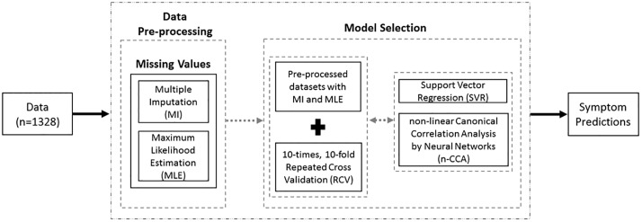
A large variety of machine learning techniques and algorithms can be used to predict data by learning from previous observations. Choosing the most appropriate one for the prediction of symptom severity is a challenging task. Several common problems exist with this type of research including: small sample sizes; a significant number of missing values; the large number of symptom assessment instruments with different measurement scales; the different types of variables (e.g., categorical, ordinal, continuous); and the subjective nature of symptom measurements, themselves. Regression analysis is a common supervised machine learning method that can be used to solve several biological and clinical problems. It is used to estimate the relationship between a dependent variable (i.e., depression, anxiety, sleep disturbance) and one or more independent variables (i.e., predictor(s)). Canonical Correlation Analysis is another analytical method for exploring the relationships between two multivariate sets of variables (e.g., set of variables from Time Point 1 (TP₁) and Time Point 2 (TP₂) of a chemotherapry (CTX) cycle). In this study, we used Support Vector Regression (SVR) with different kernels (i.e., linear, polynomial, radial sigma) and Non-linear Canonical Correlation Analysis by Neural Networks (n-CCA) [9] to predict efficiently our dependent variables (i.e., symptom severity scores of depression, anxiety and sleep disturbance at TP₂). The Multiple Imputation (MI) and Maximum Likelihood Estimation (MLE) methods were applied in order to account for missing data. Similarly, in order to accommodate the small sample size and avoid over-training, we applied a 10-times Repeated 10-fold Cross-validation (RCV) to our predictive models. To the best of our knowledge, this study is the first of its kind in oncology symptom management to applying n-CCA to predict the severity of three common symptoms in oncology patients. An overview of our analysis is provided at Fig 1.

Fig 1. Overview of our analytic approach to learn from data to predict future symptoms of oncology patients.

Our study is organized as follows: the Methods section provides the research methodology along with all of the approaches used in the proposed model. The Results section presents the comparison and evaluation of the aforementioned methods and provides a summary of our results.

Materials and methods

Study procedure

The study, from which our data was drawn, was approved by the Committee on Human Research at the University of California, San Francisco and by the Institutional Review Board at each of the study sites. From February 2010 to December 2013, all eligible patients were approached by the research staff in the infusion unit to discuss participation in the study. Written informed consent was obtained from all patients. Depending on the length of their CTX cycles, patients completed questionnaires in their homes, a total of six times over 2 cycles of CTX (i.e. prior to CTX administration (Time 1 and 4), approximately 1 week after CTX administration (Time 2 and 5), approximately 2 weeks after CTX administration (Time 3 and 6). For this study, which is a secondary analysis of existing data, symptom data from the Time 1 and Time 2 assessment were analysed. Patients were asked to report on their symptom experience for the previous week. Medical records were reviewed for disease and treatment information. The methods for the parent study are described in fully detail in previously published work. [2, 10, 11]

Patients and settings

We carried out a secondary analysis of existing data from this longitudinal study of the symptom experience of oncology outpatients receiving CTX. The data used in this study were obtained from the same dataset and relate to two different Time Points (i.e., Time Point 1 (TP₁, n₁ = 1343; prior to CTX administration), Time Point 2 (TP₂, n₂ = 1278; one week after CTX administration).

According to the study’s eligibility criteria: patients were ≥ 18 years of age; had a diagnosis of breast, gastrointestinal (GI), gynecological (GYN), or lung cancer; had received CTX within the preceding four weeks; were scheduled to receive at least two additional cycles of CTX; were able to read, write, and understand English; and gave written informed consent. Patients were recruited from two Comprehensive Cancer Centers, one Veteran’s Affairs hospital, and four community-based oncology programs.

Instruments

The study instruments included a demographic questionnaire, the Karnofsky Performance Status (KPS) scale, [12, 13] the Self-administered Comorbidity Questionnaire (SCQ), [14] the Lee Fatigue Scale (LFS), [15] the Attentional Function Index (AFI), [16, 17] the General Sleep Disturbance Scale (GSDS), [18] the Center for Epidemiological Studies-Depression Scale (CES-D), [19] and the Spielberg State-Trait Anxiety Inventories (STAI-S and STAI-T). [20]

The demographic questionnaire provided information on age, marital status, years of education, living arrangements, ethnicity, employment status and exercise. In addition patients’ medical records were reviewed to obtain information on: body mass index (BMI), hemoglobin (Hgb), type of cancer, number of metastatic sites, time since cancer diagnosis, number or prior cancer treatments, and CTX cycle length.

To estimate changes in self-reported sleep disturbance, the GSDS was administered at each time point. The GSDS consists of 21 items designed to assess the quality of sleep in the past week. Each item was rated on a 0 (never) to 7 (every day) numeric rating scale (NRS). The GSDS total score is the sum of the 21 items that can range from 0 (no disturbance) to 147 (extreme sleep disturbance). A GSDS total score of ≥ 43 indicates a significant level of sleep disturbance. [21] The GSDS has well-established validity and reliability in shift workers, pregnant women, and patients with cancer and HIV. [18, 22, 23]

The CES-D consists of 20 items selected to represent the major symptoms in the clinical syndrome of depression. Scores can range from 0 to 60, with scores ≥ 16 indicating the need for individuals to seek clinical evaluation for major depression. The CES-D has well-established concurrent and construct validity. [19, 24, 25]

The STAI-T and STAI-S inventories consist of 20 items each that are rated from 1 to 4. The scores for each scale are summed and can range from 20 to 80. A higher score indicates greater anxiety. The STAI-T measures an individual’s predisposition to anxiety determined by his/her personality and estimates how a person feels generally. The STAI-S measures an individual’s transitory emotional response to a stressful situation. It evaluates the emotional response of worry, nervousness, tension, and feelings of apprehension related to how people feel “right now” in a stressful situation. The STAI-S and STAI-T inventories have well-established criteria and construct validity and internal consistency reliability coefficients. [20, 26, 27]

Data analysis and missing data

Our data were collected from a cohort of oncology patients at two different Time Points, Time Point 1 (i.e., TP₁, n_TP1 = 1343), Time Point 2 (i.e., TP₂, n_TP2 = 1278). By merging the two different Time Points we created a new dataset of 1278 samples (n_TP1+TP2 = 1278). When we dropped the cases with at least one missing value in one of their variables, we were left with 799 cases (65,1% of n_TP1+TP2). To assess whether the missing values were missing completely at random (MCAR), missing at random (MAR), or missing not at random (MNAR) [28, 29] we analysed our data with SPSS version 23 (IBM, Armonk, NY). Furthermore, in order to avoid the problem of biasing our analysis by including only the complete cases, we used two different statistical approaches to impute the missing values, namely, Multiple Imputation (MI) [29, 30] and the Maximum Likelihood Estimation (MLE) [29, 31].

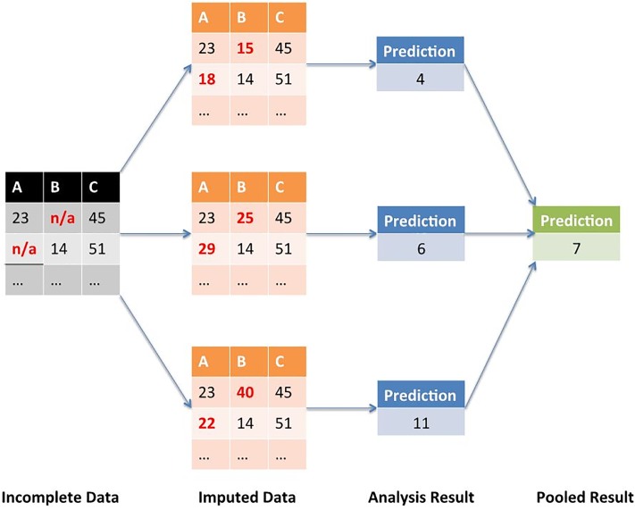
Multiple Imputation (MI) is a statistical approach to address the problem of the missing observations that are frequently encountered in all types of epidemiological and clinical studies. [32] It minimizes the uncertainty around our missing data by creating different imputed data sets several times and integrating their results into a final, pooled result. Fig 2 illustrates the MI procedure with an example.

Fig 2. Multiple imputation.

During the first stage, MI creates multiple copies of the dataset, with the missing values replaced by imputed values. These are sampled from their predictive distribution based on the observed data. [30] MI must fully account for all uncertainty in predicting the missing values by inserting appropriate variability into the multiple imputed values. During the second stage, MI fits the model of interest to each of the imputed datasets. The predicted estimations in each of the imputed datasets will differ because of the variation introduced in the imputation of the missing values. These estimates are only useful when averaged together to give the overall, pooled predicted associations.

Maximum Likelihood Estimation (MLE) is a common statistical method for estimating the parameters of a specific model, by finding the parameter values that maximize the likelihood of making the observations given these parameters. To elaborate more on this topic, [29] suppose we try an experiment with N people where the probability of a success for an individual is p and the probability of a failure is 1-p. If n people succeed and N-n people fail, the likelihood is proportional to the product of the probabilities of successes and failures or pⁿ × (1 − p)^{N − n}. The value of p that maximizes the likelihood is n/N or the overall proportion of success. In our analysis for example, maximum likelihood produces the best estimate of the difference in the parameters between TP₁ and TP₂ that maximize the probability of observing the collected data. Unlike MI, MLE provides a unique estimate of the missing values and it requires fewer decisions than MI.

To impute the missing values with the MI approach and the MLE, we used SPSS version 23 (IBM, Armonk, NY). For the MI approach, we configured SPSS to automatically choose an imputation method based on a scan of our data and produce 10 output datasets with imputed values. For the MLE approach, we configured SPSS AMOS to use an independence model with a regression imputation and produce 1 output dataset with imputed values.

Model selection

To train and evaluate the performance of our different predictive models we divided our dataset into two sub-sets: the Training (n_Train = 1000) and Validation (n_Val = 278) datasets. Cross-validation (CV) and Bootstrap are two common approaches that are known to provide unbiased estimates for the test results of a predictive model. [33] Cross-validation (CV) provides unbiased results but with a high error variance. On the other hand, Bootstrap is known to have better performance in small samples, achieving a small variance but requiring much heavier computation than CV. Combining the strengths of both approaches, Repeated Cross-validation (RCV) appears to be a good validation method for general use providing small bias with limited variability and a reasonable computation load. [33] In fact, RCV is a repeated CV method, in which the CV is repeated several times and then the average is taken. By the same rationale, Boostrap .632 is designed to address the pessimistic bias of the standard Bootstrap method, where the Bootstrap samples only contain approximately 63.2% of the unique samples from the original dataset. [34, 35]

Before training our models on the data, we empirically compared all the aforementioned validation methods on the original dataset before and after imputation for the missing values. Based on the validation method results, we compared the two different types of predictive models in our study with a 10-times and 10-fold RCV method.

We divided the original dataset with the missing values into a Training set of n_Train = 624 cases, and a Test set of n_Test = 175 cases. For the MI and MLE imputation methods, we divided the datasets into a Train set of n_Train = 1000 cases, and a Test set of n_Test = 278 cases. As already mentioned, the MI produced 10 such datasets, with each one of them having a total of n = 1278 cases.

Support Vector Regression

Support Vector Machine (SVM) is a popular machine learning algorithm used to analyze a variety of oncology data, [36–38] among many other applications. SVM became increasingly popular because of its successful application for a different set of problems (e.g. image recognition, text categorization, biosignals, bioinformatics). [39–41] SVM works by mapping data to a high-dimensional feature space so that data points can be categorized, even when the data are not otherwise linearly separable. SVM manages this challenge with an operation called the kernel trick. Through a variety of different kernel functions (e.g. Linear, Polynomial, Radial Basis Function), SVM takes low dimensional input space and transforms it to a higher dimensional space, thus converting non-separable problems to separable ones. With SVM, the data are transformed in such a way that separators between the different categories of the dataset can be found, optimized, and drawn. These separators are called the Optimal Separation Hyperplanes (OSH).

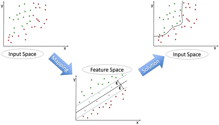
Support Vector Regression (SVR) is an extension of the SVM classifier, estimating the continuous function of a specific dataset. [42, 43] Similarly to SVM, SVR can model complex non-linear relationships by using an appropriate kernel function which maps the input data points onto a higher-dimensional feature space, transforming the non-linear relationships into linear forms. The efficiency of the procedure is determined by the kernel function’s parameters which do not depend on the dimensionality of feature space. Both SVM and SVR depend on defining a loss function, called epsilon intensive (ϵ), which ignores the errors that are situated within a certain distance of the true value. Fig 3 shows an example of a non-linear regression function with its epsilon intensive band. In our study, we implemented all the different SVR models using R version 3.3.0 and the Caret Package. [44]

Fig 3. Support Vector Regression.

Non-linear Canonical Correlation Analysis by neural networks

In our study, we adapted the n-CCA which was introduced by Hsieh et al. in 2000. [9] Our implementation was done with PyCharm Professional Edition 4.5, using Python 2.7 and the Scikit-Learn, Theano, and Lasagne libraries. [45–47]

Canonical Correlation Analysis (CCA) is a method to identify the linear combinations of a set of variables X that have the highest correlations with linear combinations of a set of variables Y. It estimates the correlated modes between the two data sets of variables X (i.e, the data from TP₁) and Y (i.e., the data from TP₂) by solving the equations,

$$\begin{array}{c}\hfill i)U=a*X,ii)V=b*Y,\end{array}$$ (1)

while maximising the Pearson correlation between U and V. To achieve a better performance in cases where the correlation between the two data sets is non-linear, the equations can be modified to include a non-linear relationship. Hsieh et al. [9] have introduced an implementation of n-CCA utilising three neural networks. For a more in-depth mathematical description of the method, we refer to the original paper. [9] In this paper, we describe the concepts of how the neural networks can be used to extract the correlation between the two sets of variables (i.e., data from TP₁ and TP₂).

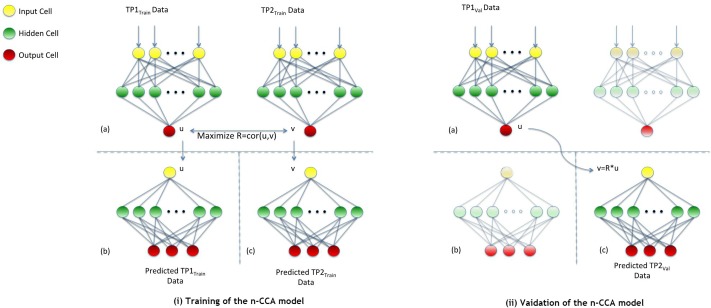
Fig 4 shows the architecture, as well as the training and validation stage, of our neural network that implements n-CCA with our data from TP₁ and TP₂. Our model consists of three networks which were trained separately. The first neural network is a double-barrelled one (illustrated in the Training-(a) section of Fig 4). We called this network the inner network and the other two the outer networks (shown in the Training-(b) and Training-(c) sections of Fig 4).

Fig 4. n-CCA training and validation: (i) training of the n-CCA model, (ii) validation of the n-CCA model.

The two barrels of the inner network (Training-(a) section of Fig 4) share the same structure and take as input the data from TP₁ and TP₂ respectively. The input layer of each barrel has n nodes, one for each feature of the data (n_Features = 29); see S1 Table for a full list of these features). The hidden layer of each barrel contains 50 nodes, that have the hyperbolic tangent function as their activation function. The output layer of each barrel has only one node, producing an output U for the dataset from TP₁ and an output V for the data set from TP₂ respectively. The aim of the training of the inner network is to maximise the correlation between the two vectors, U and V. This aim is achieved by using the negative Pearson coefficient [48] as the cost function which has to be minimised.

The outer networks (Training-(b) and Training-(c) sections of Fig 4) are trained separately, nevertheless they share the same structure. The input layer of each outer network has only one node, taking as input the output (U and V respectively) of the previous double-barrel inner network. The hidden layer of each of the outer networks has 50 nodes with the hyperbolic tangent function as their activation function. The output layer of each outer network produces the features that we need to predict. In our study, we predicted the severity of three symptoms (i.e., sleep disturbance, depression, anxiety). To predict them, each outer network learns the inverse function of each of the barrels of the inner network and maps U and V, respectively, back to the features we are interested to predict. The first outer network (Training-(b) section of Fig 4) maps U back to predicted values of sleep disturbance, depression and anxiety for TP₁ and the second outer network (Training-(c) section of Fig 4) maps V back to predicted values of sleep disturbance, depression and anxiety for TP₂. The aim of the training of the outer networks is to minimise the Mean Squared Error (MSE) between the predicted output and the true values. This training phase consists of 100 epochs, during which we used a 10-times and 10-fold RCV.

When the training stage (Training section of Fig 4) is finished, we can use parts of the model to predict TP₂ data from new, unseen TP₁ data (Validation section of Fig 4). This process can be used either to validate the model or to predict the TP₂ data, when new patients are introduced into the model, where only the TP₁ data are available. In both cases, the TP₁ data are fed into the left barrel of the inner network (Validation-(a) section of Fig 4) to estimate the U vector for these data. By multiplying this output with the Pearson coefficient R that was calculated during the training stage, we can estimate the corresponding V vector. This information forms the input for the outer right network (Validation-(c) section of Fig 4), which predicts the desired features for the TP₂ data.

Comparison between SVR and n-CCA

To compare the performances of the SVR and n-CCA models we used their Root Mean Square Error (RMSE) and Normalised Root Mean Square Error (NRMSE). The latter, was calculated by dividing their RMSE with the mean of the measured values.

$$\begin{array}{c}\hfill NRMSE=\frac{RMSE}{mean},\end{array}$$ (2)

Normalising the RMSE allows the comparison of models with different scales. Lower values among these calculations indicate less residual variance for the predicted outcomes.

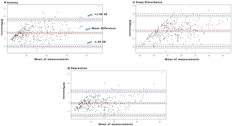
In order to compare the results produced with the SVR and the n-CCA models we used the Bland–Altman plot. [49, 50] The Bland-Altman plot is a graphical method to compare two different measurement techniques. The difference between each technique’s measurement for each case is plotted against the average of the other technique’s measurement for the same case. The former is represented on the y-axis and the latter on the x-axis. The full Bland-Altman plot draws these differences and averages for every case in the test dataset. In our study, the mean difference and the mean difference plus and minus 1.96 times the standard deviation of the differences are represented on the Bland-Altman plot with horizontal lines (see Fig 5).

Fig 5. Bland—Atman plot of the SVR model with the polynomial function and the n-CCA model on the dataset with Maximum Likelihood imputation.

In order to evaluate the agreement between the real and predicted values, we compared the mean, range, and kernel density plots of the results from the analyses on the dataset with the MLE imputation. We compared the predictions of the SVR with polynomial kernel and n-CCA models against the real values of our Test set (n_Test = 278 cases).

Results

Data analysis and handling missing data

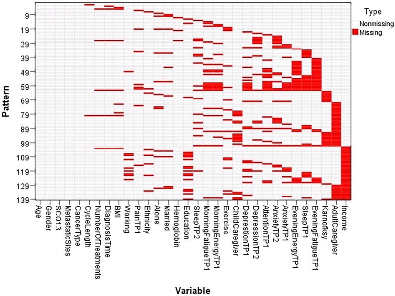
Our initial dataset that contained the data from both TP₁ (prior to CTX administration) and TP₂ (one week after CTX administration; n_TP1+TP2 = 1278), had 799 fully completed cases (65,1% of n_TP1+TP2). The empty values in the dataset were missing completely at random (Little’s MCAR test, p>0.05; Fig 6). These missing values are due to missing responses from patients. In order to use the collected values of all of our cases, we applied the MI [29, 30] and MLE [29, 31] to compensate for missing values.

Fig 6. Missing values pattern (Little’s MCAR test, p>0.05).

Model selection

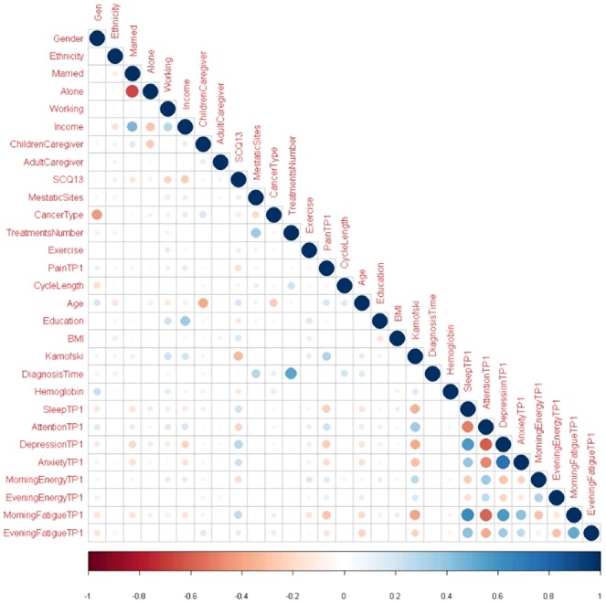
As our validation method, we selected a 10-times and 10-fold RCV. Beforehand, we compared the performance of this validation method with Bootstrap, Bootstrap .632 and 10-fold CV. As predictor variables we used the data collected from TP₁ (for a full description of these predictors see S1 Table). Moderate correlations were found among a number of predictors (see Fig 7). Type of cancer was correlated with gender because 40.6% (n = 519) of the patients in our study had breast cancer. The number of prior cancer treatments was correlated with time from patients’ initial cancer diagnosis. Income was correlated with being married and living alone. KPS score [12, 13] was moderately correlated with sleep disturbance, attentional function, depression, and morning fatigue. Finally regarding the symptoms collected in our dataset, moderate correlations were found between sleep disturbance, anxiety, depression, attentional function, morning energy, and morning fatigue.

Fig 7. Correlation analysis of predictor variables.

Our analytical models were implemented in all three types of datasets (i.e. the original ones with the missing values, the ones imputed with MI, the ones imputed with MLE). The performance of the models was evaluated based in the RMSE and the R-squared (R²). Table 1 shows the performance of different SVR models for predicting depression (CES-D) at TP₂.

Table 1. Performance of Support Vector Regression (SVR) models for predicting depression (CES-D) at TP₂.

		10-times Repeated 10-fold CV		10-fold CV		Bootstrap		Bootstrap .632
Dataset	Kernel	RMSE	R2	RMSE	R2	RMSE	R2	RMSE	R2
Missing data	Linear	6.484	0.589	6.484	0.589	6.484	0.589	6.484	0.589
	Polynomial	6.435	0.592	6.435	0.592	6.436	0.592	8.268	0.416
	Radial Sigma	6.475	0.591	6.470	0.592	6.473	0.591	6.752	0.559
Multiple Imputation	Linear	6.201	0.644	6.201	0.644	6.201	0.644	6.201	0.644
	Polynomial	6.191	0.644	6.191	0.644	6.193	0.644	8.121	0.517
	Radial Sigma	6.401	0.628	6.387	0.630	6.389	0.630	6.512	0.587
Maximum Likelihood	Linear	7.102	0.548	7.102	0.548	7.102	0.548	7.102	0.548
	Polynomial	7.081	0.549	7.081	0.549	7.053	0.552	9.954	0.323
	Radial Sigma	7.189	0.540	7.182	0.541	7.192	0.540	7.393	0.508

Based on these results (Table 1), we selected the 10-times and 10-fold RCV as our preferred validation method to test and compare the remaining analyses. The best overall performance for predicting CES-D at TP₂ with SVR was implemented with the polynomial kernel on the MI imputed dataset (RMSE = 6.191, R² = 0.644). This result could be due to the method of imputation used in the latter dataset and the type of kernel function that was used to construct the prediction model. All four validation methods provided equivalent results with their best performance implemented on the MI datasets. Bootstrap .632 combined with the polynomial kernel had the worst performance on all three types of datasets (i.e. RMSE = 9.954, R² = 0.323).

Comparison between SVR and n-CCA

To compare the different approaches used in our study, we applied three different SVR and three n-CCA models to predict the severity of depression (CES-D), sleep disturbance (GSDS), and state anxiety (STAI-S) at TP₂. The SVR models were implemented with three different kernels (i.e. Linear, Polynomial, Radial Sigma). All of our models were tested on all three types of datasets. As predictors we used all the data collected at TP₁ (see S1 Table).

We compared the performance of the models based on their RMSE, their RMSE/mean ratio (see Tables 2 & 3), and their differences in the Bland-Atman plots (Fig 5). In general the SVR models provided better fitted models with lower prediction error. All the models provided better results using the MI dataset. For the prediction of sleep disturbance, the SVR with the polynomial kernel achieved a RMSE of 13.153 and a RMSE/mean ratio of 0.209. For sleep disturbance, the n-CCA achieved a RMSE of 16.113 and R² of 0.306. For the prediction of anxiety, the polynomial kernel achieved a RMSE of 7.983 and a RMSE/mean ratio of 0.220. For anxiety the n-CCA achieved a RMSE of 8.941 and a RMSE/mean ratio of 0.677. Finally, for the prediction of depression, the polynomial kernel achieved a RMSE of 6.191 and a RMSE/mean ratio of 0.465. For depression, the n-CCA achieved a RMSE of 6.907 and a RMSE/mean ratio of 0.221.

Table 2. Performance of Support Vector Regression (SVR) models for predicting sleep disturbance (GSDS), anxiety (STAI-S) and depression (CES-D) at TP₂.

		Sleep Disturbance		Anxiety		Depression
Dataset	Kernel	RMSE	RMSE/mean	RMSE	RMSE/mean	RMSE	RMSE/mean
Missing data	Linear	13.302	0.251	8.084	0.244	6.484	0.509
	Polynomial	13.379	0.251	8.082	0.245	6.435	0.506
	Radial Sigma	13.709	0.258	8.147	0.247	6.475	0.518
Multiple Imputation	Linear	13.156	0.212	7.985	0.221	6.201	0.465
	Polynomial	13.153	0.209	7.982	0.220	6.191	0.465
	Radial Sigma	13.243	0.239	8.045	0.228	6.401	0.488
Maximum Likelihood	Linear	13.316	0.248	8.583	0.256	7.102	0.537
	Polynomial	13.331	0.246	8.476	0.251	7.081	0.536
	Radial Sigma	13.836	0.256	8.625	0.258	7.189	0.556

Table 3. Performance of n-CCA for predicting sleep disturbance (GSDS), anxiety (STAI-S) and depression (CES-D) at TP₂.

	Sleep Disturbance		Anxiety		Depression
Dataset	RMSE	RMSE/mean	RMSE	RMSE/mean	RMSE	RMSE/mean
Missing data	19.955	0.307	12.238	0.681	9.661	0.222
Multiple Imputation	16.113	0.306	8.941	0.677	6.907	0.221
Maximum Likelihood	16.680	0.305	9.320	0.676	7.583	0.218

Regarding the discrepancies between the two types of measurements as shown on the Bland-Atman plots (Fig 5), the mean differences in the measurements of all three symptoms (i.e., sleep disturbance, anxiety, depression) were close to zero. Most of these differences were between +1.96SD and -1.96SD from the mean difference, which suggests a normal distribution. The two types of analysis (i.e., SVR with polynomial kernel and n-CCA) show a moderate to high level of agreement between their measurements.

Comparison between the real and predicted values

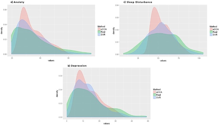
For all three symptoms (i.e., sleep disturbance, anxiety, depression), the means of the predicted values were very close to the means of the real values (Table 4). Regarding their ranges, the ranges of the predicted values from the SVR models were much closer to the ranges for the real values (Table 4). In general, the distributions of predicted values, from both analytical models, were very similar to the distributions for real values (Fig 8). n-CCA, as a Neural Network based algorithm, appears to be affected by our relatively small sample size and the distribution of data on the edges of the symptom scales. In general, it performed better where the data were denser (i.e., more data). On the other hand, SVR with polynomial kernel appears to be less affected by the aforementioned factors and provided predicted values with a high concordance with the real values.

Table 4. Sleep disturbance (GSDS), anxiety (STAI-S) and depression (CES-D) real values compared to the predicted values with the SVR (polynomial kernel) and n-CCA on the dataset with the Maximum Likelihood Estimation imputation.

Symptoms	Real Values (mean)	Real Values (range)	SVR (polynomial kernel)				n-CCA
			Predicted Values (mean)	Predicted Values (range)	RMSE	RMSE / mean	Predicted Values (mean)	Predicted Values (range)	RMSE	RMSE / mean
Sleep Disturbance	54.796	7.000 - 105.000	54.089	20.044 - 100.214	13.331	0.246	54.600	38.427 - 86.368	16.680	0.305
Anxiety	34.481	20.000 - 76.000	33.749	19.495 - 74.236	8.476	0.251	34.865	24.895 - 57.583	9.320	0.267
Depression	14.119	0.000 - 49.000	13.205	0.097 - 49.110	7.081	0.536	13.792	4.578 - 33.338	7.583	0.550

Fig 8. Density plots of the sleep disturbance (GSDS), anxiety (STAI-S) and depression (CES-D) real values compared to the density plots of predicted values with the SVR (polynomial kernel) and n-CCA on the dataset with the Maximum Likelihood Estimation imputation.

Conclusion

This study is the first to use two different machine learning techniques to accurately predict the severity of three common symptoms (i.e., sleep disturbance, anxiety, depression) from prior to through one week following the administration of CTX. The predictions were constructed using the features of the experimental dataset collected at the first Time Point. Using the SVR method, the differences between the real values (i.e., symptom severity scores that the patients reported) and the predicted values were not meaningful differences. Furthermore, we obtained fairly similar results with n-CCA at the expense of having a smaller variance among the predicted values (i.e. higher ratio of RMSE/mean in most cases). The results indicate that relatively similar findings were obtained independent of the number of missing values or the imputation method used to compensate for missing values in our dataset. The ability to predict the severity of future symptoms in oncology patients will be a powerful tool for oncology clinicians. Developing computational tools using machine learning techniques will assist clinicians to risk profile patients and implement pre-emptive symptom management interventions. Using this information, clinicians will be able to customize a patient’s treatment, increase their tolerance for CTX, and improve their quality of life. Following replication, these methods can be evaluated as a decision support tool to assist clinicians to improve symptom management in patients receiving CTX. Finally, the approaches presented in this paper, may be applicable to the same set of co-occurring symptoms in other chronic medical conditions.

The optimization of the feature selection process was one of the limitations of our study. Being an exploratory study for the performance of the aforementioned predictive models, we focused on the construction of predictive models and their evaluation and comparison. This effort was implemented through comparison of different imputation techniques (i.e. MI, MLE), validation (i.e. RCV, CV, Bootstrap, Bootstrap .632) and evaluation methods (i.e. RMSE, Bland-Altman plot). Future work will focus on defining an effective set of predictors, as well as pre-processing and enhancing the data collection and representation to improve the efficiency of both of the SVR and the n-CCA models. In addition, we will develop an incremental learning method with additional time points and evaluate it on a similar dataset. [51]

Supporting information

S1 Table. Predictor variables for the Support Vector Regression (SVR) and the Non-linear Canonical Correlation Analysis by neural networks models.

(TIF)

Data Availability

The relevant data is restricted out of consideration for patient consent and in accordance with the National Institutes of Health Data Sharing Plan. Data is available upon request to Judy Mastick (Judy.Mastick@ucsf.edu) for interested, qualified researchers.

Funding Statement

Part of this study was funded by the National Cancer Institute (CA134900). This project received funding, also, from the European Union’s Seventh Framework Programme for research, technological development and demonstration under grant agreement No 602289. Finally, this project received funding from the European Union’s Horizon 2020 research and innovation programme under grant agreement No 732679.

References

- 1. Astrup GL, Hofsø K, Bjordal K, Guren MG, Vistad I, Cooper B, et al. Patient factors and quality of life outcomes differ among four subgroups of oncology patients based on symptom occurrence. Acta Oncologica. 2017;56(3):462–470. 10.1080/0284186X.2016.1273546 [DOI] [PubMed] [Google Scholar]
- 2. Miaskowski C, Cooper B, Aouizerat B, Melisko M, Chen LM, Dunn L, et al. The symptom phenotype of oncology outpatients remains relatively stable from prior to through 1 week following chemotherapy. European journal of cancer care. 2017;26(3). 10.1111/ecc.12437 [DOI] [PMC free article] [PubMed] [Google Scholar]
- 3. Miaskowski C, Dunn L, Ritchie C, Paul SM, Cooper B, Aouizerat BE, et al. Latent class analysis reveals distinct subgroups of patients based on symptom occurrence and demographic and clinical characteristics. Journal of pain and symptom management. 2015;50(1):28–37. 10.1016/j.jpainsymman.2014.12.011 [DOI] [PMC free article] [PubMed] [Google Scholar]
- 4. Caruso R, GiuliaNanni M, Riba MB, Sabato S, Grassi L. Depressive Spectrum Disorders in Cancer: Diagnostic Issues and Intervention. A Critical Review. Current Psychiatry Reports. 2017;19(6):33 10.1007/s11920-017-0785-7 [DOI] [PMC free article] [PubMed] [Google Scholar]
- 5. Kyranou M, Paul SM, Dunn LB, Puntillo K, Aouizerat BE, Abrams G, et al. Differences in depression, anxiety, and quality of life between women with and without breast pain prior to breast cancer surgery. European Journal of Oncology Nursing. 2013;17(2):190–195. 10.1016/j.ejon.2012.06.001 [DOI] [PMC free article] [PubMed] [Google Scholar]
- 6. Gold M, Dunn LB, Phoenix B, Paul SM, Hamolsky D, Levine JD, et al. Co-occurrence of anxiety and depressive symptoms following breast cancer surgery and its impact on quality of life. European Journal of Oncology Nursing. 2016;20:97–105. 10.1016/j.ejon.2015.06.003 [DOI] [PMC free article] [PubMed] [Google Scholar]
- 7. Dahiya S, Ahluwalia MS, Walia HK. Sleep disturbances in cancer patients: underrecognized and undertreated. Cleveland Clinic journal of medicine. 2013;80(11):722–732. 10.3949/ccjm.80a.12170 [DOI] [PubMed] [Google Scholar]
- 8. Alvaro PK, Roberts RM, Harris JK. A systematic review assessing bidirectionality between sleep disturbances, anxiety, and depression. Sleep. 2013;36(7):1059–1068. 10.5665/sleep.2810 [DOI] [PMC free article] [PubMed] [Google Scholar]
- 9. Hsieh WW. Nonlinear canonical correlation analysis by neural networks. Neural Networks. 2000;13(10):1095–1105. 10.1016/S0893-6080(00)00067-8 [DOI] [PubMed] [Google Scholar]
- 10. Wright F, Hammer M, Paul SM, Aouizerat BE, Kober KM, Conley YP, et al. Inflammatory pathway genes associated with inter-individual variability in the trajectories of morning and evening fatigue in patients receiving chemotherapy. Cytokine. 2017;91:187–210. 10.1016/j.cyto.2016.12.023 [DOI] [PMC free article] [PubMed] [Google Scholar]
- 11. Kober KM, Cooper BA, Paul SM, Dunn LB, Levine JD, Wright F, et al. Subgroups of chemotherapy patients with distinct morning and evening fatigue trajectories. Supportive care in cancer: official journal of the Multinational Association of Supportive Care in Cancer. 2016;24(4):1473 10.1007/s00520-015-2895-2 [DOI] [PMC free article] [PubMed] [Google Scholar]
- 12. Karnofsky D. Performance scale. Factors that influence the therapeutic response in cancer: A comprehensive treatise. 1977; p. 97–101. [Google Scholar]
- 13. Da K, Abelman W, Craver L, Burchenal J. The use of nitrogen mustards in the palliative tratment of cancer. Cancer. 1948;1:634–6456. [Google Scholar]
- 14. Sangha O, Stucki G, Liang MH, Fossel AH, Katz JN. The self-administered comorbidity questionnaire: a new method to assess comorbidity for clinical and health services research. Arthritis Care & Research. 2003;49(2):156–163. 10.1002/art.10993 [DOI] [PubMed] [Google Scholar]
- 15. Lee KA, Hicks G, Nino-Murcia G. Validity and reliability of a scale to assess fatigue. Psychiatry research. 1991;36(3):291–298. 10.1016/0165-1781(91)90027-M [DOI] [PubMed] [Google Scholar]
- 16. Cimprich B. Attentional fatigue following breast cancer surgery. Research in nursing & health. 1992;15(3):199–207. 10.1002/nur.4770150306 [DOI] [PubMed] [Google Scholar]
- 17. Chen ML, Miaskowski C, Liu LN, Chen SC. Changes in perceived attentional function in women following breast cancer surgery. Breast cancer research and treatment. 2012;131(2):599–606. 10.1007/s10549-011-1760-3 [DOI] [PubMed] [Google Scholar]
- 18. Lee KA. Self-reported sleep disturbances in employed women. Sleep. 1992;15(6):493–498. 10.1093/sleep/15.6.493 [DOI] [PubMed] [Google Scholar]
- 19. Radloff LS. The CES-D scale: A self-report depression scale for research in the general population. Applied psychological measurement. 1977;1(3):385–401. 10.1177/014662167700100306 [DOI] [Google Scholar]
- 20. Spielberger C, Gorsuch R, Suchene R, Vagg P, Jacobs G. Manual for the State-Anxiety (Form Y): Self Evaluation Questionnaire. Palo Alto, CA: consulting psychologists press; 1970;. [Google Scholar]
- 21. Fletcher BS, Paul SM, Dodd MJ, Schumacher K, West C, Cooper B, et al. Prevalence, severity, and impact of symptoms on female family caregivers of patients at the initiation of radiation therapy for prostate cancer. Journal of Clinical Oncology. 2008;26(4):599–605. 10.1200/JCO.2007.12.2838 [DOI] [PubMed] [Google Scholar]
- 22. Lee KA, DeJoseph JF. Sleep disturbances, vitality, and fatigue among a select group of employed childbearing women. Birth. 1992;19(4):208–213. 10.1111/j.1523-536X.1992.tb00404.x [DOI] [PubMed] [Google Scholar]
- 23. Miaskowski C, Lee KA. Pain, fatigue, and sleep disturbances in oncology outpatients receiving radiation therapy for bone metastasis: a pilot study. Journal of pain and symptom management. 1999;17(5):320–332. [DOI] [PubMed] [Google Scholar]
- 24. Sheehan TJ, Fifield J, Reisine S, Tennen H. The measurement structure of the Center for Epidemiologic Studies Depression scale. Journal of personality assessment. 1995;64(3):507–521. 10.1207/s15327752jpa6403_9 [DOI] [PubMed] [Google Scholar]
- 25. Carpenter J, Andrykowski M, Wilson J, Hall L, Kay Rayens M, Sachs B, et al. Psychometrics for two short forms of the Center for Epidemiologic Studies-Depression Scale. Issues in mental health nursing. 1998;19(5):481–494. 10.1080/016128498248917 [DOI] [PubMed] [Google Scholar]
- 26. Bieling PJ, Antony MM, Swinson RP. The State–Trait Anxiety Inventory, Trait version: structure and content re-examined. Behaviour research and therapy. 1998;36(7):777–788. 10.1016/S0005-7967(98)00023-0 [DOI] [PubMed] [Google Scholar]
- 27. Kennedy BL, Schwab JJ, Morris RL, Beldia G. Assessment of state and trait anxiety in subjects with anxiety and depressive disorders. Psychiatric Quarterly. 2001;72(3):263–276. [DOI] [PubMed] [Google Scholar]
- 28. Little RJ, Rubin DB. Statistical analysis with missing data. John Wiley & Sons; 2014. [Google Scholar]
- 29. Dziura JD, Post LA, Zhao Q, Fu Z, Peduzzi P. Strategies for dealing with missing data in clinical trials: from design to analysis. The Yale journal of biology and medicine. 2013;86(3):343 [PMC free article] [PubMed] [Google Scholar]
- 30. Sterne JA, White IR, Carlin JB, Spratt M, Royston P, Kenward MG, et al. Multiple imputation for missing data in epidemiological and clinical research: potential and pitfalls. Bmj. 2009;338:b2393 10.1136/bmj.b2393 [DOI] [PMC free article] [PubMed] [Google Scholar]
- 31. Enders CK. A primer on maximum likelihood algorithms available for use with missing data. Structural Equation Modeling. 2001;8(1):128–141. 10.1207/S15328007SEM0801_7 [DOI] [Google Scholar]
- 32. van der Heijden GJ, Donders ART, Stijnen T, Moons KG. Imputation of missing values is superior to complete case analysis and the missing-indicator method in multivariable diagnostic research: a clinical example. Journal of clinical epidemiology. 2006;59(10):1102–1109. 10.1016/j.jclinepi.2006.01.015 [DOI] [PubMed] [Google Scholar]
- 33. Kim JH. Estimating classification error rate: Repeated cross-validation, repeated hold-out and bootstrap. Computational statistics & data analysis. 2009;53(11):3735–3745. 10.1016/j.csda.2009.04.009 [DOI] [Google Scholar]
- 34. Efron B. Estimating the error rate of a prediction rule: improvement on cross-validation. Journal of the American statistical association. 1983;78(382):316–331. 10.1080/01621459.1983.10477973 [DOI] [Google Scholar]
- 35. Efron B, Tibshirani R. Improvements on cross-validation: the 632+ bootstrap method. Journal of the American Statistical Association. 1997;92(438):548–560. 10.1080/01621459.1997.10474007 [DOI] [Google Scholar]
- 36. Chu F, Wang L. Applications of support vector machines to cancer classification with microarray data. International journal of neural systems. 2005;15(06):475–484. 10.1142/S0129065705000396 [DOI] [PubMed] [Google Scholar]
- 37. Wang H, Huang G. Application of support vector machine in cancer diagnosis. Medical oncology. 2011;28(1):613–618. 10.1007/s12032-010-9663-4 [DOI] [PubMed] [Google Scholar]
- 38.Nandpuru HB, Salankar S, Bora V. MRI brain cancer classification using support vector machine. In: Electrical, Electronics and Computer Science (SCEECS), 2014 IEEE Students’ Conference on. IEEE; 2014. p. 1–6.
- 39. Bennett KP, Campbell C. Support vector machines: hype or hallelujah? Acm Sigkdd Explorations Newsletter. 2000;2(2):1–13. 10.1145/380995.380999 [DOI] [Google Scholar]
- 40. Nilashi M, Ibrahim O, Ahani A. Accuracy improvement for predicting Parkinson’s disease progression. Scientific reports. 2016;6 10.1038/srep34181 [DOI] [PMC free article] [PubMed] [Google Scholar]
- 41. Xu C, Qu H, Wang G, Xie B, Shi Y, Yang Y, et al. A novel strategy for forensic age prediction by DNA methylation and support vector regression model. Scientific reports. 2015;5. [DOI] [PMC free article] [PubMed] [Google Scholar]
- 42. Basak D, Pal S, Patranabis DC. Support vector regression. Neural Information Processing-Letters and Reviews. 2007;11(10):203–224. [Google Scholar]
- 43. Smola AJ, Schölkopf B. A tutorial on support vector regression. Statistics and computing. 2004;14(3):199–222. 10.1023/B:STCO.0000035301.49549.88 [DOI] [Google Scholar]
- 44. Kuhn M. Caret package. Journal of Statistical Software. 2008;28(5):1–26.27774042 [Google Scholar]
- 45. Pedregosa F, Varoquaux G, Gramfort A, Michel V, Thirion B, Grisel O, et al. Scikit-learn: Machine learning in Python. Journal of Machine Learning Research. 2011;12(Oct):2825–2830. [Google Scholar]
- 46.Dieleman S, Schlüter J, Raffel C, Olson E, Sønderby SK, Nouri D, et al. Lasagne: First release.; 2015. Available from: 10.5281/zenodo.27878. [DOI]
- 47.Theano Development Team. Theano: A Python framework for fast computation of mathematical expressions. arXiv e-prints. 2016;abs/1605.02688.
- 48. Mukaka MM. A guide to appropriate use of correlation coefficient in medical research. Malawi Medical Journal. 2012;24(3):69–71. [PMC free article] [PubMed] [Google Scholar]
- 49. Altman DG, Bland JM. Measurement in medicine: the analysis of method comparison studies. The statistician. 1983; p. 307–317. 10.2307/2987937 [DOI] [Google Scholar]
- 50. Hanneman SK. Design, analysis and interpretation of method-comparison studies. AACN advanced critical care. 2008;19(2):223 10.1097/01.AACN.0000318125.41512.a3 [DOI] [PMC free article] [PubMed] [Google Scholar]
- 51. Maguire R, Fox PA, McCann L, Miaskowski C, Kotronoulas G, Miller M, et al. The eSMART study protocol: a randomised controlled trial to evaluate electronic symptom management using the advanced symptom management system (ASyMS) remote technology for patients with cancer. BMJ open. 2017;7(5):e015016 10.1136/bmjopen-2016-015016 [DOI] [PMC free article] [PubMed] [Google Scholar]
Associated Data
This section collects any data citations, data availability statements, or supplementary materials included in this article.
Supplementary Materials
(TIF)
Data Availability Statement