In Silico Assessment of Literature Insulin Bolus Calculation Methods Accounting for Glucose Rate of Change

Abstract

Background:

The standard formula (SF) used in bolus calculators (BCs) determines meal insulin bolus using “static” measurement of blood glucose concentration (BG) obtained by self-monitoring of blood glucose (SMBG) fingerprick device. Some methods have been proposed to improve efficacy of SF using “dynamic” information provided by continuous glucose monitoring (CGM), and, in particular, glucose rate of change (ROC). This article compares, in silico and in an ideal framework limiting the exposition to possibly confounding factors (such as CGM noise), the performance of three popular techniques devised for such a scope, that is, the methods of Buckingham et al (BU), Scheiner (SC), and Pettus and Edelman (PE).

Method:

Using the UVa/Padova Type 1 diabetes simulator we generated data of 100 virtual subjects in noise-free, single-meal scenarios having different preprandial BG and ROC values. Meal insulin bolus was computed using SF, BU, SC, and PE. Performance was assessed with the blood glucose risk index (BGRI) on the 9 hours after meal.

Results:

On average, BU, SC, and PE improve BGRI compared to SF. When BG is rapidly decreasing, PE obtains the best performance. In the other ROC scenarios, none of the considered methods prevails in all the preprandial BG conditions tested.

Conclusion:

Our study showed that, at least in the considered ideal framework, none of the methods to correct SF according to ROC is globally better than the others. Critical analysis of the results also suggests that further investigations are needed to develop more effective formulas to account for ROC information in BCs.

One of the most cumbersome tasks in the daily management of type 1 diabetes (T1D) is the calculation of the amount of insulin to be injected at meal-time. To help T1D patients in this process, bolus calculators (BCs) are available, integrated in insulin pumps, as stand-alone devices, and in the form of mobile apps.¹ Commonly, to estimate the insulin bolus amount B (U) needed to compensate for the intake of a certain quantity of carbohydrates (CHO) (g), BCs implement the following standard formula (SF):

$$B=\frac{CHO}{CR}+\frac{G_c-G_T}{CF}-IOB$$ (1)

where CR and CF are, respectively, the carbohydrate-to-insulin ratio (g/U) and the correction factor (mg/dL/U) (two patient-specific therapy parameters which are tuned-up by physicians using empirical laws based on experience),² G_C is the measured preprandial blood glucose (BG) concentration (mg/dL), G_T is the target BG level (mg/dL); and IOB is the so-called insulin on board (U) (an estimate of how much insulin is still acting in the organism from the previous boluses).³ It was shown that BCs implementing the SF (1) generally improve BG control,^3-4 even if optimal CR and CF values may vary with time of the day according to patient intraday physiologic variability and the CHO estimation is affected by uncertainty,⁵ factors that can lead to suboptimal glycemic outcome after the meal.

The SF (1) uses only “static” information on BG, as it was developed when standard BG monitoring was performed by self-monitoring of blood glucose (SMBG) fingerprick devices. More recently, continuous glucose monitoring (CGM) sensors were introduced and some of them received the regulatory approval for nonadjunctive use,^6,7 that is, their measurements can be used for decision-making and, in particular, insulin bolus calculation, without the need of confirmatory SMBG. In a nonadjunctive CGM scenario, the SF can still be used by simply substituting the SMBG measurement with the CGM value at the time of bolus calculation. However, CGM sensors provide information about the current glucose rate of change (ROC) that could be useful for a better determination of the amount of insulin to inject.^8-10 Indeed, some methods were proposed in the literature to “adjust” the SF (1) by exploiting ROC arrows information, including those of Buckingham et al,¹¹ Scheiner,¹² and Pettus and Edelman,¹³ hereafter labeled as SC, PE, and BU, respectively. To the best of our knowledge, no study has quantitatively evaluated the performance of these methods yet. In this work, we perform such an investigation in silico, in a single meal scenario, by using the UVa/Padova T1D simulator.¹⁴ In particular, we analyze data of 100 virtual subjects with different preprandial BG and ROC values. We assess the performance of each method by calculating the blood glucose risk index (BGRI) on the 9 hours after the meal. Comparison among the three methods is performed in an ideal noise-free framework, the aim being limiting, at this stage of the investigation, the influence of possibly confounding factors (such as errors in carb counting, sensor readings, etc).

Methods

Literature Methods for Adjustment of Insulin Bolus According to ROC

The BU method, proposed in 2008,¹¹ consists in modulating the SF (1) according to ROC magnitude and direction. In detail, patients are suggested to increase/decrease insulin bolus by 10% when CGM sensor reports that BG is rising/decreasing by 1-2 mg/dL/min. Otherwise, if BG is changing by 2-3 mg/dL/min or more, patients are advised to increase or decrease insulin bolus by 20%.

The SC guideline, proposed in 2015,¹² suggests using ROC as a tool to infer the glucose levels over the next 30-60 minutes, assuming that the current glucose trend will be stable by the time the insulin starts to act. In particular, the BG measurement used in (1), that is, G_C, is substituted by its predicted value according to ROC. In practice, if BG is increasing/decreasing by 1-3 mg/dL/min, the patient is suggested to “adjust” G_C by summing/subtracting 25 mg/dL to it. Otherwise, if BG is changing by 3 mg/dL/min or more, the patient is advised to increase or decrease G_C by 50 mg/dL.

Recent studies investigating how patients employ CGM and ROC to make insulin therapy adjustments revealed that people are inclined to make more drastic and extreme changes than those suggested by both BU and SC guidelines.^9,10 For example, when G_C is 110 mg/dL and BG is rapidly increasing, T1D patients reported to increase the insulin bolus by 81% instead of just 20%. In line with these findings, the PE guideline was proposed in 2017,¹³ which uses the same rationale of SC but suggests larger G_C corrections. In particular, the PE method consists in increasing/decreasing the measured glucose concentration by 50 mg/dL, 75 mg/dL, and 100 mg/dL when glucose is changing by 1-2 mg/dL/min, 2-3 mg/dL/min, and more than 3 mg/dL/min, respectively. See Table 1 for a summary of the BU, SC, and PE methods.

Table 1.

Comparison of the Literature Guidelines for the Adjustment of the Insulin Bolus B Computed in (1).

ROC indication	BU11	SC12	PE13
Constant: glucose is steady or is not decreasing/increasing by more than 1 mg/dL/min	B* = B	GC* = GC	GC* = GC
Slowly rising: glucose is rising by 1-2 mg/dL/min	B* = B + 10%	GC* = GC + 25	GC* = GC + 50
Rising: glucose is rising by 2-3 mg/dL/min	B* = B + 20%	GC* = GC + 25	GC* = GC + 75
Rapidly rising: glucose is rising by more than 3 mg/dL/min	B* = B + 20%	GC* = GC + 50	GC* = GC + 100
Slowly falling: glucose is falling 1-2 mg/dL/min	B* = B − 10%	GC* = GC − 25	GC* = Gc − 50
Falling: glucose is falling 2-3 mg/dL/min	B* = B − 20%	GC* = GC − 25	GC* = GC − 75
Rapidly falling: glucose is falling more than 3 mg/dL/min	B* = B − 20%	GC* = GC − 50	GC* = GC − 100

B* and G_C* are the adjusted insulin bolus and the corrected BG measurement, respectively.

Simulation Framework

To evaluate and compare the performance of BU, SC, and PE against SF (considered as reference) we designed an ad hoc in silico clinical trial using the UVa/Padova T1D simulator.¹⁴ We performed the trial in 100 virtual adults having (mean ± SD) body weight 69.7 ± 12.4 kg, total daily insulin 0.61 ± 0.18 U/day/kg, CR 15.9 ± 5.3 g/U, fasting plasma glucose 119.6 ± 6.7 mg/dL (we refer the reader to Dalla Man et al¹⁴ for more details). Each subject underwent 9-hour single-meal experiments. The simulation started at 12:00 pm, when the subjects had a lunch of 75g of CHO, and ended at 21:00 pm. We studied each subject in different scenarios characterized by different BG and ROC values at meal time, with the aim of assessing the impact of preprandial conditions, in terms of BG and ROC, on BC’s performance. In particular, we designed these scenarios by a trial-and-error approach, in which we tuned time and CHO content of breakfast and morning snack and time and amount of the respective insulin boluses to achieve the desired (BG, ROC) condition at meal time. In total, we generated 24 different scenarios, deriving from the combination of four preprandial ROC intervals, that is, −3 to −2, −2 to −1, 1 to 2, and 2 to 3 mg/dL/min, and six preprandial BG intervals, that is, 60 ± 5, 70 ± 5, 80 ± 5, 100 ± 5, 150 ± 5, and 250 ± 5 mg/dL. Note that we decided not to test scenarios where preprandial ROC is between −1 and 1 mg/dL/min, since BU, SC, and PE do not correct the SF for these ROC values. We also decided not to test scenarios with extreme preprandial ROC values, that is, ROC > 3 mg/dL/min and ROC < −3 mg/dL/min, since impossible to simulate in all the subjects with realistic manipulations of time, CHO content and insulin bolus of breakfast and morning snack.

To assess the performance of each BC method per se, we decided to limit the exposition of the study to possibly confounding factors (eg, patient behavior in making treatment decisions to mitigate hyper/hypoglycemia, changes in individual insulin sensitivity, low or high preprandial insulin/carbohydrate on board amount, CGM errors and artifacts that can also alter the estimation of the ROC value) and run the simulations in a noise free environment, that is, using optimal therapy parameters, allowing neither postprandial correction boluses nor hypotreatments, without simulating errors in meal CHO counting, BG measurement and ROC estimation.

Performance Evaluation and Statistical Analysis

For each subject and each (BG, ROC) pairs, we compared the BG profile obtained using the SF, that is, when the bolus dose is calculated by using the “static” BG value at meal-time, with the BG profiles obtained from the adoption of the three literature methods which include in (1) the “dynamic” information provided by the CGM sensor, that is, the ROC. Note that, for each particular meal condition scenario, we discarded those virtual subjects whose insulin bolus computed with SF resulted to be zero or negative (eg, because of too much elevated IOB values), since in such a situation the methods would not be comparable.

The quality of glucose control was assessed, first of all, by calculating BGRI in the postprandial 9-h time window.¹⁵ This metric, thanks to the glucose scale symmetrization, is equally sensitive to hypoglycemia and hyperglycemia and condenses glycemic excursions in a single quantity, facilitating interpretation and comparison of the results. To evaluate the between-methods differences, the two-tailed Wilcoxon signed-rank test with 1% significance was performed. In particular, we applied the Bonferroni correction for multiple comparisons, thus dividing the significance level by the total number of comparisons we made. To assess whether or not some patient characteristics can impact the outcome, for each scenario we computed the Spearman’s correlation coefficient between body weight (BW), total daily insulin (TDI), basal insulin infusion rate (Ib), G_T, CR, CF, IOB, and the BGRI difference (ΔBGRI) between BU versus SF, SC versus SF, and PE versus SF. The statistical significance of the obtained correlation was evaluated using as significance level α = 1%.

Finally, to give a picture of the relative performance of the three methods more focused on hypoglycemia, we computed, for each subject, the low blood glucose risk index (LBGI),¹⁵ a metric that, besides quantifying the risk for hypoglycemia, incorporates information on duration and severity of the event). Specifically, we considered LBGI obtained using the methods BU, SC, and PE under comparison and the LBGI obtained using SF, and we calculated the respective average ratio.

Results

Figure 1 presents two examples of BG traces obtained using both ROC-modified BC literature methods and SF. Top panel represents adult 6 with preprandial BG 100 ± 5 mg/dL and ROC −3 to −2 mg/dL/min. In this case adjusting the original insulin bolus amount according to ROC allows to achieve a better glucose control both during and after the meal, reducing and even zeroing (when using PE) time spent in hypoglycemia. In particular, PE correction is the one that performs best (BGRI(SF) = 6.39, BGRI(BU) = 5.00, BGRI(SC) = 3.84, BGRI(PE) = 1.81). The second example, reported in the bottom panel, represents adult 20 with preprandial BG 150 ± 5 mg/dL and ROC 2 to 3 mg/dL/min. This case presents worse glycemic outcomes compared to SF when applying either SC, PE, and BU correction (BGRI(SF) = 7.80, BGRI(BU) = 13.86, BGRI(SC) = 9.14, BGRI(PE) = 14.93) which drive the virtual subject to hypoglycemia.

Figure 1.

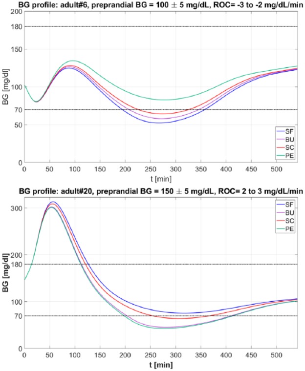
Example of BG trace obtained with SF (in blue), BU (in violet), SC (in red), PE (in green), and BU (in violet) methods. Top panel. BG profiles obtained for the virtual subject adult 6 when preprandial ROC is −3 to −2 mg/dL/min and preprandial BG is 100 ± 5 mg/dL. Bottom panel. BG profiles obtained for the virtual subject adult 20 when ROC is 2 to 3 mg/dL/min and preprandial BG is 150 ± 5 mg/dL.

Below, for each of the considered ROC intervals, we analyze and compare the obtained glycemic outcomes resulting from the adoption of SF, BU, SC, and PE in the virtual population.

ROC −3 to −2 mg/dL/min

In Figure 2A, the distributions of the ΔBGRI between BU versus SF, SC versus SF, and PE versus SF obtained in all the 100 virtual subjects when preprandial ROC is −3 to −2 mg/dL/min are shown via boxplot representation. According to Figure 2A, all methods improve significantly the BGRI (P < .01) obtained with SF. This is visible also in Table 2, where we report the median/interquartile range of the BGRI distribution obtained using SF, BU, SC, and PE. However, the boxplots in Figure 2A also evidence that several subjects obtained worse glycemic outcomes when the dose is corrected according to either BU, SC, or PE compared to SF.

Figure 2.

Boxplot representation of the distribution of ΔBGRI obtained comparing BU versus SF (in blue), SC vs SF (in red), PE versus SF (in green) when ROC is −3 to −2 mg/dL/min (panel A), −2 to −1 mg/dL/min (panel B), 1 to 2 mg/dL/min (panel C), and 2 to 3 mg/dL/min (panel D). Red horizontal lines represent median, boxes mark interquartile ranges, dashed lines are the whiskers, red crosses indicate outliers. Black stars indicate statistical significant between-distribution differences. Lower ΔBGRI means better glucose control quality.

Table 2.

BGRI Results Obtained for Different Preprandial BG Level When ROC Is −3 to −2 mg/dL/min (Panel A), −2 to −1 mg/dL/min (Panel B), 1 to 2 mg/dL/min (Panel C), and 2 to 3 mg/dL/min (Panel D).

		Preprandial BG (mg/dL)
		60 ± 5	70 ± 5	80 ± 5	100 ± 5	150 ± 5	250 ± 5
(A) ROC = −3 to −2 mg/dL/min	SF	14.72 [6.85-27.47]	12.84 [4.86-21.67]	13.91 [5.09-31.16]	12.88 [5.03-30.58]	8.03 [5.12-21.45]	10.91 [7.93-21.71]
	BU	11.45 [5.35-22.88]	8.63 [5.13-18.49]	9.25 [4.84-26.15]	9.10 [4.97-26.94]	7.86 [5.17-15.92]	10.53 [7.44-16.26]
	SC	12.23 [5.54-23.84]	7.95 [3.98-18.70]	10.09 [4.58-26.19]	9.01 [4.97-26.66]	7.77 [5.04-17.85]	10.29 [7.28-17.67]
	PE	10.95 [5.18-20.86]	7.55 [4.00-17.00]	9.18 [4.49-24.59]	8.36 [5.01-25.16]	7.70 [4.97-15.14]	9.80 [7.22-15.28]
(B) ROC −2 to −1 mg/dL/min	SF	5.51 [3.77-13.07]	5.88 [3.74-13.72]	5.70 [3.75-15.57]	6.50 [3.95-20.64]	5.92 [4.61-9.62]	10.56 [7.95-15.06]
	BU	5.39 [3.96-10.09]	5.60 [3.77-10.85]	5.68 [3.62-13.08]	6.75 [4.08-18.15]	6.26 [4.23-8.96]	9.96 [7.92-14.51]
	SC	5.20 [4.03-10.02]	5.68 [3.87-11.50]	5.61 [3.65-12.41]	6.23 [3.90-17.35]	6.07 [4.31-8.61]	10.31 [7.81-14.00]
	PE	5.15 [4.03-9.70]	5.31 [3.89-9.61]	5.31 [3.81-10.40]	5.74 [4.11-13.95]	6.13 [4.34-8.38]	9.90 [7.95-13.67]
(C) ROC = 1 to 2 mg/dL/min	SF	9.15 [6.81-12.28]	8.07 [6.27-10.99]	7.52 [5.82-10.95]	8.98 [6.56-11.35]	10.16 [8.25-12.60]	14.30 [11.19-20.77]
	BU	8.45 [6.36-11.78]	7.54 [5.57-10.15]	7.21 [5.57-9.65]	8.51 [6.21-10.59]	9.79 [7.57-12.93]	14.26 [11.19-20.77]
	SC	8.38 [6.42-12.05]	7.66 [5.84-10.38]	7.32 [5.66-10.03]	8.59 [6.19-10.98]	9.85 [7.77-13.56]	14.49 [10.86-21.82]
	PE	8.17 [6.21-11.28]	7.63 [5.52-9.82]	7.40 [5.27-9.93]	8.53 [6.02-10.68]	9.67 [7.63-13.39]	14.28 [11.47-21.63]
(D) ROC 2 to 3 mg/dL/min	SF	16.99 [11.85-22.01]	13.11 [9.81-17.89]	12.34 [9.24-17.47]	11.03 [8.40-16.21]	13.65 [9.52-18.71]	16.89 [12.70-20.80]
	BU	14.58 [10.70-19.21]	11.48 [8.49-15.42]	10.66 [8.15-15.00]	9.93 [7.57-14.98]	12.88 [8.99-18.21]	16.43 [12.24-21.39]
	SC	14.72 [10.56-19.05]	11.24 [8.59-15.46]	10.37 [8.37-15.18]	9.89 [7.82-15.77]	13.54 [8.78-19.38]	16.54 [12.81-21.65]
	PE	14.14 [10.36-18.09]	11.08 [8.41-15.69]	10.94 [8.08-15.98]	9.96 [7.60-15.25]	13.11 [9.38-19.55]	15.95 [12.58-23.27]

Median [interquartile range] reported for BGRI obtained with the considered literature methods (BU, SC, and PE) and the SF.

In Figure 3A, we report the boxplot representation of the ΔBGRI distributions obtained by comparing SC versus BU, PE versus BU, and PE versus SC when preprandial ROC is −3 to −2 mg/dL/min. Indeed, except for preprandial BG 150 ± 5 mg/dL where all methods achieve equivalent performance, PE obtained significantly (P < .01) better BGRI values compared to both BU and SC. Furthermore, as visible in Table 2A, comparing SC versus BU, better BGRI are achieved using BU.

Figure 3.

Boxplot representation of the distribution of ΔBGRI obtained comparing SC versus BU (in gray), PE versus BU (in violet), and PE versus SC (in green) when ROC is −3 to −2 mg/dL/min (panel A), −2 to −1 mg/dL/min (panel B), 1 to 2 mg/dL/min (panel C), and 2 to 3 mg/dL/min (panel D). Red horizontal lines represent median, boxes mark interquartile ranges, dashed lines are the whiskers, red crosses indicate outliers. Black stars indicate statistical significant between-distribution differences. Lower ΔBGRI means better glucose control quality.

As far as the correlation analysis is concerned, comparing BU, SC, and PE with the SF, we find that, when ROC is −3 to −2 mg/dL/min, the respective ΔBGRI are weakly but significantly correlated (P < .01) with CR and IOB. No significant correlation has been found for the other considered patients’ parameters.

Table 3A reports the average ratio between the LBGI obtained using the considered methods and the LBGI obtained using the SF when ROC is −3 to −2 mg/dL/min. Results show that, as expected, the LBGI decreases using BU, SC, and PE, as the computed insulin bolus amount decreases as well. In particular, PE achieves lower ratios, being the most conservative.

Table 3.

Mean (SD) Ratio Between the LBGI Obtained Using the Considered Methods (BU, SC, and PE) and the LBGI Obtained Using the SF Results Are Obtained for Different Preprandial BG Level When ROC Is −3 to −2 mg/dL/min (Panel A), −2 to −1 mg/dL/min (Panel B), 1 to 2 mg/dL/min (Panel C), and 2 to 3 mg/dL/min (Panel D).

		Preprandial BG (mg/dL)
		60 ± 5	70 ± 5	80 ± 5	100 ± 5	150 ± 5	250 ± 5
(A) ROC = −3 to −2 mg/dL/min	BU – SF	0.84 (0.16)	0.83 (0.19)	0.83 (0.20)	0.85 (0.18)	0.78 (0.22)	0.70 (0.24)
	SC – SF	0.83 (0.16)	0.82 (0.18)	0.81 (0.20)	0.84 (0.17)	0.80 (0.19)	0.73 (0.22)
	PE – SF	0.77 (0.20)	0.77 (0.22)	0.76 (0.24)	0.79 (0.21)	0.74 (0.24)	0.65 (0.27)
(B) ROC −2 to −1 mg/dL/min	BU – SF	0.88 (0.14)	0.87 (0.14)	0.87 (0.14)	0.87 (0.14)	0.83 (0.17)	0.76 (0.18)
	SC – SF	0.88 (0.15)	0.87 (0.15)	0.87 (0.14)	0.87 (0.14)	0.83 (0.17)	0.81 (0.14)
	PE – SF	0.79 (0.23)	0.78 (0.23)	0.78 (0.22)	0.79 (0.21)	0.73 (0.25)	0.68 (0.23)
(C) ROC = 1 to 2 mg/dL/min	BU – SF	1.13 (0.21)	1.17 (0.26)	1.21 (0.32)	1.21 (0.30)	1.33 (0.40)	1.56 (0.61)
	SC – SF	1.13 (0.24)	1.16 (0.27)	1.19 (0.31)	1.19 (0.32)	1.25 (0.40)	1.25 (0.32)
	PE – SF	1.44 (0.84)	1.52 (0.93)	1.61 (1.06)	1.62 (1.10)	1.78 (1.48)	1.64 (0.90)
(D) ROC 2 to 3 mg/dL/min	BU – SF	1.19 (0.49)	1.27 (0.54)	1.42 (0.76)	1.53 (0.83)	1.93 (1.34)	2.73 (2.16)
	SC – SF	1.21 (0.55)	1.29 (0.70)	1.40 (0.84)	1.47 (0.95)	1.72 (1.47)	1.62 (0.86)
	PE – SF	1.50 (1.20)	1.75 (1.75)	1.97 (1.12)	2.10 (1.55)	2.52 (2.18)	2.21 (1.89)

ROC −2 to −1 mg/dL/min

Figure 2B shows the distributions of ΔBGRI obtained by comparing the considered methods against SF when preprandial ROC is −2 to −1 mg/dL/min. In this situation, the outcomes are strongly dependent on the specific preprandial BG level. Indeed, although all methods allowed obtaining statistically significant better performance than SF for preprandial BG 80 ± 5, 100 ± 5 and 250 ± 5 mg/dL, there are no statistically significant (P < .01) differences when comparing BU, SC, and PE versus SF for preprandial BG 60 ± 5 and 150 ± 5 mg/dL, and PE versus SF for preprandial BG 70 ± 5 mg/dL. Considering the median results (see Table 2), the best outcomes were achieved without adjusting the reference insulin bolus when preprandial BG is 150 ± 5 mg/dL and using PE for the other preprandial BG conditions.

As shown in Figure 2B, the fact that the considered methods do not perform better than SF is due to the presence of a nonnegligible number of subjects whose BGRI is higher when using BU, SC, and PE. Moreover, such a worsening of BGRI is more pronounced if larger corrections are applied to SF, like using the PE guideline. Indeed, the bigger the correction of SF, the higher the variability obtained in terms of BGRI.

Figure 3B shows the ΔBGRI distributions obtained comparing the considered methods between each other. In these scenarios we cannot detect any statistically significant difference between the methods.

Furthermore, the correlation analysis obtains same qualitative results as ROC −3 to −2 mg/dL/min. Specifically, comparing BU versus SF, SC versus SF, and PE versus SF when ROC is −2 to −1 mg/dL/min, we find weak but significant correlation (P < .01) between ΔBGRI and CR and IOB.

Table 3B reports the average ratio between the LBGI obtained using the considered methods and the LBGI obtained using the SF when ROC is −2 to −1 mg/dL/min. Results show same qualitative outcomes as ROC −3 to −2 mg/dL/min. Specifically, average LBGI decreases when BU, SC, and PE are adopted.

ROC 1 to 2 mg/dL/min

Figure 2C reports, via boxplot representation, the ΔBGRI distributions obtained comparing BU, SC, and PE versus SF. In this case, adjusting insulin bolus according to ROC we almost always obtained better results in terms of glycemic control. In particular, best median BGRI values (see Table 2) are achieved using PE for preprandial BG 60 ± 5 and 150 ± 5 mg/dL, BU for preprandial BG 70 ± 5, 80 ± 5, and 250 ± 5 mg/dL and SC for preprandial BG 100 ± 5 mg/dL. However, when preprandial BG is 250 ± 5 mg/dL there is no statistically significant difference between BU, SC, and PE and SF, due to a substantial degradation of the glucose control performance in almost half of the considered subjects when a correction is applied to SF.

Focusing on the between-methods comparison (see Figure 3C), results suggest that, when preprandial BG is 150 ± 5 mg/dL, the best outcomes are achieved by the PE indication. On the other hand, when preprandial BG is 250 ± 5 mg/dL, the best results are obtained using BU. Notably, SC presents worse BGRI results compared to both BU and PE, in all of the considered scenarios. Furthermore, as reported in Table 2C, comparing SC versus BU, better BGRI are achieved using the latter.

Concerning the correlation analysis results, comparing BU versus SF, SC versus SF, and PE versus SF when ROC is 1 to 2 mg/dL/min, we find that ΔBGRI is significantly correlated (P < .01) with BW and G_T. No significant correlation has been found for the other considered patients’ parameters.

Finally, in Table 3C we report the average ratio between the LBGI obtained using the considered methods and the LBGI obtained using the SF when ROC is 1 to 2 mg/dL/min. Again, these results are not surprising, since BU, SC, and PE increase the insulin bolus amount when ROC >0. Specifically, higher ratios are obtained using the PE method, since it implements the most aggressive adjustment of the SF.

ROC 2 to 3 mg/dL/min

Figure 2D shows the ΔBGRI distributions obtained by comparing the considered correction methods against SF. Results show that adjusting the reference insulin bolus according to ROC significantly (P < .01) improved, on average, the glycemic outcomes. In particular, best median BGRI results (see Table 2) are achieved using PE for preprandial BG 60 ± 5, 70 ± 5, and 250 ± 5 mg/dL, SC for preprandial BG 80 ± 5 and 100 ± 5 mg/dL and BU for preprandial BG 150 ± 5 mg/dL. However, there are no statistically significant differences comparing BU, SC, and PE versus SF when preprandial BG is 250 ± 5 mg/dL, since correcting SF leads to a degradation of the glycemic outcomes in a consistent part of the population.

In Figure 3D we show the ΔBGRI distributions of SC versus BU, PE versus BU, and PE versus SC via boxplot representation. Results show that BU and PE get almost the same performance and outperform SC when preprandial BG is 150 ± 5 mg/dL. On the other hand, when preprandial BG is 250 ± 5 mg/dL, PE and SC are not significantly different from each other and the best results are achieved using BU.

Finally, as far as the correlation analysis is concerned, we find that, comparing BU, SC, and PE with the SF when ROC is 2 to 3 mg/dL/min, ΔBGRI is significantly correlated (P < .01) with BW, G_T and CR.

Table 3D reports the average ratio between the LBGI obtained using the considered methods and the LBGI obtained using the SF when ROC is 2 to 3 mg/dL/min. Results show the same qualitative results as ROC 1 to 2 mg/dL/min.

Discussion and Conclusion

Methods for BC that can take advantage of the “dynamic” information provided by CGM sensors and, in particular, of the ROC have been recently proposed. The most popular are BU, SC, and PE. To the best of our knowledge, no study has quantitatively evaluated them yet. In this article, we compared these three methods and assessed their performance in noise-free single meal in silico scenarios.

Our results showed that, overall, none of the considered approaches clearly prevails on the others, since the best modulation of the insulin bolus results strongly related to preprandial conditions. In the scenarios in which preprandial BG is rapidly decreasing (ROC −3 to −2 mg/dL/min), we observed the best performance for PE which allowed reducing the insulin bolus amount more than the other methods, thus resulting in better glycemic outcome. When BG is slightly decreasing (ROC −2 to −1 mg/dL/min), none of the three “dynamic” methods is superior for all the preprandial BG levels tested. The same comment applies to positive ROC scenarios, in which in particular no statistically significant BGRI improvement was obtained by either SC, BU and PE compared to SF when BG was 250 ± 5 mg/dL. Finally, our results showed that the none of the methods to correct SF according to ROC performs well in all the subjects. Indeed, even if all the methods achieved significantly better results in median BGRI compared to SF, this improvement was not achieved for all the subjects, with several subjects obtaining worse glycemic outcomes when either BU, SC, or PE were applied. In particular, our results show an important limitation of BU, SC, and PE. In fact, when ROC is positive, the risk for hypoglycemia systematically increases even if, following the intuition, the increased amount of administered insulin should compensate the positive ROC without inducing hypoglycemia.

In conclusion, it is important to remark that the comparison of methods documented in this work was performed in an ideal noise-free framework, the aim being limiting the influence of possibly confounding factors, such as errors in patient behavior,¹⁶ carb miscalculations, sensor readings, and so on, that, however, should be carefully considered in the continuation of this research.

As far as future work is concerned, the present article suggests that using CGM trend information for insulin dosing requires particular attention. Indeed, although having information about ROC can potentially improve the current SF for insulin bolus calculation, the rules for integrating ROC information in BC must be carefully devised and comprehensively assessed to ensure their safety. Therefore, further investigations are needed to design new BCs able to effectively take advantage of the “dynamic” information on BG available from CGM. In particular, new methodologies should personalize the correction of (1) taking into account also the subject’s characteristics, as proposed by Aleppo et al¹⁷ (who suggested to add/subtract a fixed amount of insulin to SF considering not only the glucose ROC, but also the patient insulin sensitivity) and Cappon et al¹⁸ (who investigated the use of neural networks in tackling insulin bolus personalization). Indeed, our results follow this direction, that is, showing weak but significant correlation between the obtained glycemic outcomes and some of the patient’s specific parameters. Specifically, our analysis suggests that, when ROC is negative, the insulin bolus dose should be modulated exploiting also CR and the IOB amount instead of just ROC. On the other hand, when ROC is positive, results indicates that BW, G_T and CR should also be accounted in the adjustment of the SF. Of course, any new algorithm will also have to demonstrate its robustness in more challenging in silico scenarios incorporating perturbations and sources of error not considered in the conceptual evaluation done in the present article.

References

- 1. Schmidt S, Norgaard K. Bolus calculators. J Diabetes Sci Technol. 2014;8:1035-1041. [DOI] [PMC free article] [PubMed] [Google Scholar]
- 2. Davidson PC, Hebblewhite HR, Steed RD, Bode BW. Analysis of guidelines for basal-bolus insulin dosing: basal insulin, correction factor and carbohydrate-to-insulin ratio. Endocr Prat. 2008;14:1095-1101. [DOI] [PubMed] [Google Scholar]
- 3. Gross TM, Kayne D, King A, Rother C, Juth S. A bolus calculator is an effective means of controlling postprandial glycemia in patients on insulin pump therapy. Diabetes Technol Ther. 2003;10:365-369. [DOI] [PubMed] [Google Scholar]
- 4. Klonoff DC. The current status of bolus calculator decision-support software. J Diabetes Sci Technol. 2012;6:990-994. [DOI] [PMC free article] [PubMed] [Google Scholar]
- 5. Marden S, Thomas PW, Sheppard ZA, Knott J, Lueddeke J, Kerr D. Poor numeracy skills are associated with glycaemic control in Type 1 diabetes. Diabetic Med. 2012;29:662-669. [DOI] [PubMed] [Google Scholar]
- 6. Edelman SV. Regulation catches up to reality nonadjunctive use of continuous glucose monitoring data. J Diabetes Sci Technol. 2017;1:160-164. [DOI] [PMC free article] [PubMed] [Google Scholar]
- 7. US Food and Drug Administration. Dexcom G5 Mobile Continuous Glucose Monitoring System. Available at: https://www.accessdata.fda.gov/cdrh_docs/pdf12/P120005S041a.pdf. Accessed October 20, 2017.
- 8. Juvenile Diabetes Research Foundation Continuous Glucose Monitoring Study Group. Continuous glucose monitoring and intensive treatment of type 1 diabetes. N Engl J Med. 2008;359:1464-1476. [DOI] [PubMed] [Google Scholar]
- 9. Hirsch IB. Clinical review: realistic expectations and practical use of continuous glucose monitoring for the endocrinologist. J Clin Endocrinol Metab. 2009;94:2232-2238. [DOI] [PubMed] [Google Scholar]
- 10. Pettus J, Edelman SV. Use of glucose rate of change arrows to adjust insulin therapy among individuals with type 1 diabetes who use continuous glucose monitoring. Diabetes Technol Ther. 2016;18:S2-S34. [DOI] [PMC free article] [PubMed] [Google Scholar]
- 11. Buckingham B. Use of the direcnet applied treatment algorithm (data) for diabetes management with a real-time continuous glucose monitor (the FreeStyle Navigator). Pediatr Diabetes. 2008;9:142-147. [DOI] [PMC free article] [PubMed] [Google Scholar]
- 12. Scheiner G. Practical CGM: Improving Patient Outcomes Through Continuous Glucose Monitoring. Alexandria, WV: American Diabetes Association; 2015. [Google Scholar]
- 13. Pettus J, Edelman SV. Recommendations for using real-time continuous glucose monitoring (rtCGM) data for insulin adjustments in type 1 diabetes. J Diabetes Sci Technol. 2017;11:138-147. [DOI] [PMC free article] [PubMed] [Google Scholar]
- 14. Dalla Man C, Micheletto F, Lv D, Breton M, Kovatchev B, Cobelli C. The UVa/Padova type 1 diabetes simulator: new features. J Diabetes Sci Technol. 2014;8:26-34. [DOI] [PMC free article] [PubMed] [Google Scholar]
- 15. Fabris C, Patek SD, Breton MD. Are risk indices derived from CGM interchangeable with SMBG-based indices? J Diabetes Sci Technol. 2016;10:50-59. [DOI] [PMC free article] [PubMed] [Google Scholar]
- 16. Vettoretti M, Facchinetti A, Sparacino G, Cobelli C. Type 1 diabetes patient decision simulator for in silico testing safety and effectiveness of insulin treatments. IEEE Trans Biomed Eng 2018;65(6):1281-1290. [DOI] [PubMed] [Google Scholar]
- 17. Aleppo G, Laffel LM, Ahmann AJ, et al. A practical approach to using trend arrows on the Dexcom G5 CGM system for the management of adults with diabetes. J Endocr Soc. 2017;1:1-16. [DOI] [PMC free article] [PubMed] [Google Scholar]
- 18. Cappon G, Vettoretti M, Marturano F, Facchinetti A, Sparacino G. A neural network based approach to personalize insulin bolus calculation using continuous glucose monitoring. J Diabetes Sci Technol. 2018;12:265-272. [DOI] [PMC free article] [PubMed] [Google Scholar]