Estimating the evolution of disease in the Parkinson’s Progression Markers Initiative

Abstract

Parkinson’s disease is the second most common neurological disease and affects about one percent of persons above the age of 60. Due to the lack of approved surrogate markers, confirmation of the disease still requires post-mortem examination. Identifying and validating biomarkers are essential steps toward improving clinical diagnosis and accelerating the search for therapeutic drugs to ameliorate disease symptoms. Until recently, statistical analysis of multi-cohort longitudinal studies of neurodegenerative diseases has usually been restricted to a single analysis per outcome with simple comparisons between diagnostic groups. However, an important methodological consideration is to allow the modeling framework to handle multiple outcomes simultaneously and consider the transitions between diagnostic groups. This enables researchers to monitor multiple trajectories, correctly account for the correlation among biomarkers, and assess how these associations may jointly change over the long-term course of disease. In this study, we apply a latent time joint mixed-effects model to study biomarker progression and disease dynamics in the Parkinson’s Progression Markers Initiative (PPMI) and examine which markers might be most informative in the earliest phases of disease. The results reveal that, even though diagnostic category was not included in the model, it seems to accurately reflect the temporal ordering of disease state consistent with diagnosis categorization at baseline. In addition, results indicated that Specific Binding Ratio (SBR) on striatum and Total Unified Parkinson Disease Rating Scale (UPDRS), show high discriminability between disease stages. An extended latent time joint mixed-effects model with heterogeneous latent time variance also showed improvement in model fit in a simulation study and when applied to real data.

1. Introduction

Parkinson’s disease (PD) affects nearly 1% of persons above the age of 60. Degeneration and death of neurons in the substantia nigra of the brain occurs much earlier than the onset of motor symptoms such as slow movement, tremor, and rigidity. Disease progression is characterized by the transition from normal, through preclinical, to clinical stages of the disease. Confirmation of the disease is only possible through an autopsy. Presence of non-motor symptoms such as olfactory, sleep and depression help classify patients as prodromal since there is currently no available surrogate marker to confirm disease diagnosis. Currently, the FDA approves DaTscan, a specialized imaging technique of the brain that measures levels of dopamine in the substantia nigra, to evaluate suspected PD. Nonetheless, diagnosis of the onset and progression of the disease is often marred by errors due to the unavailability of reliable validated diagnostic markers. Identifying and validating biomarkers are crucial steps in clinical diagnosis and the search for treatment to ameliorate disease symptoms and slow down the progression of PD. Reliable and cost-effective biomarkers for the diagnosis of neurodegenerative diseases are more likely to be discovered if multiple clinical, biological and imaging assessments are studied simultaneously to provide complementary information.

In studies of neurodegenerative diseases such as PD, clinical, biological and imaging biomarkers are often collected longitudinally over a short period of time on individuals at different stages of disease. Such studies are aimed at accurately characterizing disease trajectories and identifying important diagnosis and prognosis biomarkers, and ultimately help to accelerate drug discovery. Although studies generally collect multiple outcomes over time, it is very common to find studies where researchers focus on the analysis of changes in a single outcome. In this regard, the linear mixed-effects model is ubiquitous in studies of neurodegenerative diseases. For example, Kennedy et al. (2015) applied linear mixed effect models to estimate rate of decline of Alzheimer’s Disease Assessment Scale Cognitive score (ADASCog) among AD patients based on Mini Mental State Examination (MMSE). Guerrero et al. (2016) reported studies which employ mixed-effect models for the analysis of longitudinal AD markers. Mixed-effect models are also commonly applied in the Parkinson’s disease literature. Sturkenboom et al. (2014) assessed the effect of occupational therapy on Canadian Occupational Performance measure in improving the daily activity of PD patients. Klotsche et al. (2011) analyzed changes in health-related quality of life (HRQoL) in a longitudinal cohort study of PD patients. Analysis of single longitudinal outcomes can be inefficient for studying the progression of the disease since outcomes may be correlated and hence may provide complementary insights. Single-outcome analyses may also contribute to the lack of strong evidence of symptomatic or disease-modifying treatment effects on clinical outcomes. Inference may be improved if all outcomes are modelled simultaneously, taking into account the intra- and inter-subject variability and accommodating between outcomes associations.

Joint models that simultaneously model two or more outcomes have received relatively less attention in the neurodegenerative disease literature. This neglect is likely due to problems in interpretation of resulting parameter estimates, or to the computational complexities that arise when the number of outcomes grows or when the outcomes are of mixed types, such as binary, count, continuous, or time-to-event. Moreover, in most studies, which do employ multivariate models, only two outcomes are modelled at a time (Iddi & Molenberghs (2012); Tsiatis & Davidian (2004)). Nevertheless, the multivariate modeling framework offers several potential advantages, such as accommodating all sources of variation and correlation among outcomes. With the rapid emergence and growing popularity of Bayesian estimation methods to handle complex and computationally burdensome models, multivariate modelling techniques have become an active area of research in neurodegenerative studies. Luo & He (2016) analyzed longitudinal outcomes and a time-to-event outcome to assess the effect of tocopherol on patients with early PD using a Bayesian Markov Chain Monte Carlo (MCMC) method for the efficient estimation of model parameters. Their modeling framework applied a multilevel item response theory model for multiple longitudinal outcomes and a Cox proportional hazard model for the survival outcome. They demonstrated that their joint model led to a better fit to their data than single analyses per outcome. Luo (2014) provides an excellent review of recent developments and issues of joint modeling of longitudinal and survival data. Li et al. (2017) proposed a latent time joint mixed effect model (LTJMM), an extension of the multivariate linear mixed effects model for longitudinal data, which accommodates a large number of outcomes to be analyzed together and permits unbalanced time measurement of outcomes. A distinctive feature of this model is the inclusion of a latent time shift parameter, which captures the degree of an individual’s disease progression. The subject-specific latent times shared across outcomes are assumed to have a homogeneous variance across all subjects.

In this study, we extended the LTJMM by relaxing the homogeneity assumption on the latent times. Heterogeneity was introduced by allowing the latent time to be influenced by subject-level covariates. To achieve this, we modelled the latent time variance in terms of covariates through an exponential function. The heterogeneous latent time joint mixed effects model was used to estimate trajectories of biomarkers and determine the sequence of biomarker abnormality using data from the Parkinson’s Progression Markers Initiative (PPMI) study. Estimation of model parameters was via a Bayesian MCMC framework.

2. Materials and Methods

2.1. Data

The Parkinson’s Progression Markers Initiative (PPMI) is a prospective multi-center study of patients at different stages of Parkinson disease (PD) with healthy patients as controls. Roughly 35 centers across North America, Europe, Israel, and Australia are involved in this ongoing study that has collected data over a period of 6 years. All study sites received institutional review board approval before initiating the study, and all study participants provided written informed consent for research. Detailed study design, inclusion criteria, standard protocols, registration and consent procedures can be found on the study website (www.ppmi-info.org). The study is aimed at identifying novel clinical, imaging and biologic markers of Parkinson’s disease and to assess their progression in patients. Discovery and validation of new biomarkers would be beneficial for use in clinical trials of disease-modifying drugs. Patients are classified by their disease stage, namely Healthy Controls (HC), Parkinson’s Disease (PD), Scan without evidence of dopaminergic deficit (SWEDD), Prodromal, Genetic cohort and Genetic Registry patients. The genetic cohort and registry subjects may or may not be affected with Parkinson’s symptoms. The steps involved in diagnosing and classifying participants into disease categories are reported in the PPMI study protocol.

In this study, we focused on subjects in the HC, PD and Prodromal groups. There were 475 PD, 238 HC, and 187 Prodromal individuals representing 52.78%, 26.44%, and 20.78% of the sample, respectively. Of these participants, 317 (35.22%) were female and 583 (64.78%) were male. The proportion of females in the HC, PD and Prodromal groups was 34.87%, 35.58%, and 34.76% respectively. Visit times were not balanced, as the schedule of assessments depended on the group. Healthy controls were followed every 6 months for the first year and 12 months thereafter. Before the first 12 months, PD and Prodromal patients were followed every 3 months and for every 6 months thereafter.

We considered 17 outcomes and modelled 8 of them using age and gender as covariates. Clinical assessments included Tremor, Postural Instability and Gait Difficulty (PIGD), REM sleep behavior disorder (RBD), University of Pennsylvania Smell Identification Test (UPSIT), Montreal Cognitive Assessment (MOCA), Hopkins Verbal Learning Test (HVLT), Geriatric Depression Scale (GDS), Semantic Fluency Test (SFT), Movement Disorder Society Unified Parkinson Disease Rating Scale (MDS-UPDRS), Total Scale for Outcomes in Parkinson’s (SCOPA), Line Orientation Test (LINEORT), Montreal Cognitive Assessment (MOCA) and State Trait Anxiety Index (STAI). UPDRS total includes the 3 subtests; UPDRS I gauges mentation, behavior, and mood, UPDRS II assesses activities of daily living and UPDRS III examines motor. To complement these clinical outcomes, we also investigated biologic markers such as cerebrospinal fluid (CSF) alpha-synuclein (α-syn), CSF Amyloid peptide 42 (Aβ42), CSF phosphorylated tau 181 p (p-tau181) and CSF Total tau (t-tau). These outcomes have long been known to be associated with the development and progression of Parkinson’s disease. We also included DAT Scan summaries of the striatum.

2.2. Statistical Methods

We employed the latent time joint mixed-effect model (LTJMM) to assess the relationship between CSF measures, imaging biomarkers, and the clinical outcomes and further explore its use to study progression among diagnostic groups. The LTJMM allows for multiple outcomes, measured longitudinally for each patient potentially at different visit times. Suppose y_ijk represents the outcome k (k = 1, 2, …, p) observed at time j (j = 1, …, q) for each individual, i (i = 1, 2, …, n), t_ij is the time of measurement, and x_ijk is a set of covariates for the ith individual at time j. The model is given by

$$Y_{ijk}={\mathit{x}}_{ijk}^t{\mathit{\beta }}_k+{\gamma }_k(t_{ij}+{\delta }_i)+{\alpha }_{0ik}+{\alpha }_{1ik}{t}_{ij}+{\epsilon }_{ijk},$$

where β_k and γ_k are coefficients corresponding to covariates and time, respectively, α_0ik and α_1ik are subject-specific random intercept and slope components specific to each outcome and assumed to follow a multivariate normal distribution with mean 0 and variance-covariance matrix, D. A random or “latent” time-shift, δ_i specific to each subject but shared across all outcomes is introduced to quantify the disease progression of an individual relative to the population. The δ_i are assumed to follow a normal distribution with mean 0 and variance ${\sigma }_{\delta }^2$. Finally, the independent random error term, ε_ijk is assumed to follow a normal distribution with mean, 0 and variance, σ². Additionally, δ_i is assumed to be independent of the subject-specific random effects and the pure random errors. However, the subject-specific random intercepts and slopes are allowed to be correlated to reflect the dependence among outcomes. Heterogeneity in the latent time (LTJMM-H) is introduced by modeling ${\sigma }_{\delta }^2$ as follows:

$${\sigma }_{{\delta }_i}^2=\exp \left({\mathit{Z}}_i^t\mathit{\tau }\right),$$

where Z_i represents a set of covariates for individual i assumed to be a subset of X_i and τ is a vector of parameters corresponding to the covariates. With this, we have allowed the variability of the latent time to vary across subjects.

To efficiently estimate the model parameters, an MCMC approach was adopted. We assign a weakly informative normal prior with zero mean and variance 100 on the regression and γ_k parameters. For the variance components of the time shift and random error term, a weakly informative half-Cauchy (0, 2.5) distribution was imposed. For the subject-specific random effects, the variance-covariance matrix was first decomposed into variance and correlation components. A Cholesky decomposition was then applied to the correlation matrix to ensure efficiency and stability. A half-Cauchy(0, 25) prior was placed on the variance part and the LKJ prior on the correlation matrix as recommended by Lewandowski et al. (2009). To ensure identifiability of the model, we constrained the random intercepts for each subject to sum to zero (i.e, ${\sum }_{k=1}^p{\alpha }_{0ik}=0$).

3. Simulation Study

A limited simulation study was conducted to study the effect of assuming a homogeneous latent time variance when in fact there is between-subject variation in latent time variance. We generated data from the LTJMM-H model with uncorrelated random effects as follows:

$$y_{ijk}={\beta }_{0k}+{\beta }_{1k}{x}_{1ijk}+{\beta }_{2k}{x}_{2ijk}+{\gamma }_k\left(t_{ij}+{\delta }_i\right)+{\alpha }_{0ik}+{\alpha }_{1ik}+{\epsilon }_{ijk},$$

where i = 1,2, …, 5, x_1ijk~bin(0.5), x_2ijk~N(55, 5²), α_0ik and α_1ik are random intercept and slope, respectively and assumed to be independent. Further,

$$\log \left({\sigma }_{{\delta }_i}^2\right)={\tau }_0+{\tau }_1{x}_{1i}+{\tau }_2{x}_{2i}$$

The sample size was set to 100 with each individual time, t_ijk~Uniform(0,6).

Simulation parameters were set by fitting the LTJMM model to five of the original outcomes in the PPMI study. Heterogeneity was introduced by allowing a small effect of x_1i and x_2i in the sub-model. Actual parameter values for both fixed effects and variance components can be seen in Table 1. We then simulated 100 datasets and fitted both the LTJMM and the LTJMM-H with correlated random-effects to the data. To apply the MCMC algorithm, we specified two Markov chains, each run for 2000 iteration including 1000 warm-up iterations, which were discarded. Simulation results are presented in Table 1. Both models consistently estimated fixed parameters, variance parameters of the random-effects and the random error with high coverage probability. However, the LTJMM performed poorly in the estimation of the latent-time variance resulting in severe bias and zero coverage probability for the true parameters. Also, the LTJMM-H model resulted in smaller WAIC and LOOIC in many of our simulations, demonstrating better model fit compared to LTJMM.

Table 1:

Simulation study results. One hundred simulated data sets were generated under model LTJMM (independent random effects). Both LTJMM-Het and LTJMM models with correlated random effects were fit to all simulated data sets. The best performance was determined by the lowest WAIC and LOOIC between the two models for each data and summarized as “% best” over the 100 simulations. Bias and 95% Coverage Probabilities are also reported for each parameter.

Model Parameters	True Values	LTJMM-Het Model		LTJMM Model
		Bias	Coverag	Bias	Coverage
β0	−31.7	1.6929	0.86	1.7119	0.86
β1	−2.06	0.1139	0.94	0.0957	0.98
β2	0.12	−0.0314	0.9	−0.0312	0.88
β0	−30.70	0.8346	0.93	0.8408	0.93
β1	0.52	0.0138	0.97	0.0072	0.95
β2	0.06	−0.0156	0.93	−0.0154	0.92
β0	−7.60	1.3147	0.97	1.3778	0.98
β1	3.90	0.3746	0.95	0.3227	0.98
β2	0.28	−0.031	0.98	−0.0304	0.96
β0	17.20	−0.5776	1.00	−0.399	1.00
β1	−1.56	1.1918	0.98	1.0105	0.98
β2	0.08	−0.0145	1.00	−0.0114	1.00
β0	−36.20	8.2043	0.74	8.2752	0.73
β1	−1.40	0.3505	0.97	0.2837	0.97
β2	0.18	−0.1564	0.68	−0.1553	0.74
γ1	0.15	0.0106	0.96	0.0105	0.97
γ2	0.09	0.0064	0.98	0.0063	0.98
γ3	0.60	0.0461	0.96	0.0457	0.94
γ4	2.20	0.1588	0.97	0.1576	0.95
γ5	0.80	0.0577	0.98	0.0573	0.97
σα01	3.20	−0.0548	0.96	−0.0574	0.96
σα02	1.60	−0.021	0.97	−0.0203	0.97
σα03	5.60	−0.0224	0.95	−0.0218	0.95
σα04	7.10	0.0800	0.96	0.0781	0.95
σα11	0.60	−0.007	0.90	−0.0054	0.9
σα12	0.47	0.0209	0.93	0.0214	0.94
σα13	1.17	0.0022	0.96	0.0033	0.97
σα14	3.70	−0.1244	0.92	−0.1267	0.91
σα15	5.70	0.0657	0.96	0.0657	0.96
σ1	3.10	0.0198	0.93	0.0200	0.93
σ2	1.60	0.0229	0.97	0.0226	0.95
σ3	4.80	0.0556	0.95	0.0552	0.97
σ4	5.80	0.0601	0.94	0.0602	0.94
σ5	1.60	−6e-04	0.96	−2e-04	0.97
τ0	3.60	−0.1314	0.95	2.1513	0.00
τ1	−1.50	0.0131	0.97	-	-
τ2	0.05	2e-04	0.95	-	-
% best WAIC	61%
% best LOOIC	63%

4. Analysis of PPMI

4.1. Exploratory Analysis

Table 2 summarizes patient characteristics and outcomes at baseline in the PPMI dataset. Using ANOVA, the diagnostic groups at baseline yielded significant difference in means, with all p-values < 0.05. The average age was higher in the prodromal group compared to HC and PD categories. Tremor, one of the main clinical manifestations of PD, was unsurprisingly higher on average among PD patients relative to the other diagnostic groups.

Table 2:

Summary measures at baseline.

Diagnostic Category	Variable	n	Min	Max	Mean	SE
HC	Age	199	30.54	83.87	60.79	0.80
	CSF Abeta 42	190	88.80	879.50	377.62	8.22
	CSF Alpha-synuclein	190	592.56	8608.91	2201.26	78.86
	CSF p-Tau181P	190	5.10	73.30	18.22	0.85
	CSF Total tau	188	18.40	223.10	52.48	1.98
	GDSSHORT	199	0.00	15.00	1.29	0.15
	HVLT	198	15.00	35.00	26.02	0.32
	LINEORNT	198	4.00	15.00	13.14	0.14
	PIGD	198	0.00	0.80	0.02	0.01
	REM Sleep	198	0.00	11.00	2.86	0.17
	SCOPA	197	0.00	35.00	8.10	0.52
	SFT	198	22.00	80.00	51.90	0.80
	STAI	196	40.00	105.00	57.08	1.00
	Tremor	197	0.00	0.64	0.03	0.01
	UPDRS Total	197	0.00	20.00	4.63	0.32
	UPSIT	199	10.00	40.00	33.89	0.36
Prodromal	Age	64	58.37	82.12	68.75	0.73
	HVLT	63	9.00	33.00	21.79	0.67
	LINEORNT	62	3.00	15.00	11.97	0.29
	PIGD	63	0.00	0.60	0.10	0.02
	REM Sleep	63	1.00	14.00	7.54	0.48
	SCOPA	64	1.00	39.00	15.50	1.22
	SFT	63	26.00	75.00	45.00	1.37
	Tremor	63	0.00	0.45	0.08	0.02
	UPDRS Total	63	0.00	31.00	12.32	0.99
	UPSIT	61	7.00	35.00	17.18	0.84
PD	Age	430	33.63	84.71	61.57	0.47
	CSF Abeta 42	416	129.20	796.50	370.82	4.91
	CSF Alpha-synuclein	416	332.93	6694.55	1847.87	38.72
	CSF p-Tau181P	414	4.70	94.10	15.74	0.50
	CSF Total tau	412	14.40	121.00	44.80	0.91
	GDSSHORT	428	0.00	14.00	2.32	0.12
	HVLT	426	9.00	36.00	24.47	0.24
	LINEORNT	426	5.00	15.00	12.78	0.10
	PIGD	411	0.00	1.40	0.23	0.01
	REM Sleep	416	0.00	13.00	4.50	0.14
	SCOPA	430	0.00	71.00	12.55	0.45
	SFT	426	20.00	103.00	48.79	0.57
	STAI	425	40.00	137.00	65.25	0.89
	Tremor	411	0.00	1.82	0.50	0.02
	UPDRS Total	406	7.00	76.00	32.52	0.67
	UPSIT	427	1.00	40.00	22.29	0.40

Abbreviations: PIGD, Posture Instability and Gait Difficulty; RBD, REM sleep behavior disorder; UPSIT, University of Pennsylvania Smell Identification Test; MOCA, Montreal Cognitive Assessment; HVLT, Hopkins Verbal Learning Test; GDS, Geriatric Depression Scale; SFT, Semantic Fluency Test; SCOPA, Scale for Outcomes in Parkinson’s; LINEORT, Line Orientation Test; UPDRS, Unified Parkinson Disease Rating Scale; STAI, State Trait Anxiety Index; PD, Parkinson Disease; HC, Healthy Control; SE, Standard Error.

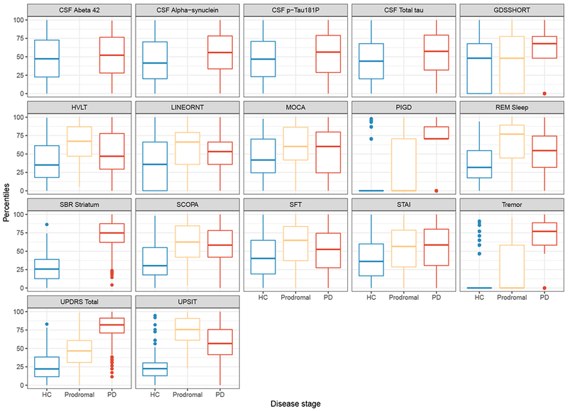
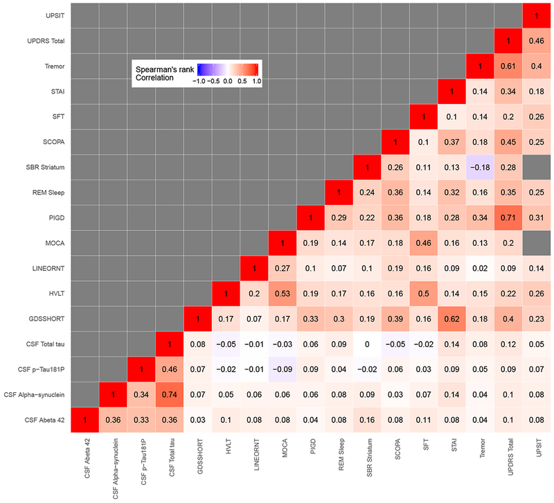
To compare outcomes on a common scale, raw scores were transformed into percentiles using a weighted empirical cumulative distribution function. The inverse of the sample proportion of diagnostic category for each outcome was used as weights. Table 3 shows percentile scores corresponding to selected percentile ranks. Figure 1a shows the boxplot of the percentile ranks, representing disease severity, for each outcome in each of the three diagnostic categories. From this figure, we observe broad variation in percentile ranks of the outcomes for each disease group. There were outlying observations, particularly for the motor outcomes, tremor, PIGD and UPDRS total and olfactory measures indexed by UPSIT. The median ranks differ among diagnostic groups and were lowest in the HC group. The Spearman rank correlations between outcomes are displayed in a heat map in Figure 1b. Total tau was highly correlated with CSF alpha-synuclein (r = 0.74). PIGD was also strongly associated with UPDRS total (r = 0.71). Generally, motor outcomes were highly correlated. CSF biomarkers were also generally correlated with each other but weakly associated with clinical outcomes. A cognitive outcome, MOCA, was moderately positively correlated with verbal working memory assessment indexed by HVLT (r = 0.53), and depression (GDS) was moderately correlated with anxiety (STAI) with r = 0.62.

Table 3:

Percentiles and percentile ranks of outcomes.

Outcomes	Min	25th	50th	75th	Max
Tremor	0.00	0.05	0.12	0.43	2.36
PIGD	0.00	0.07	0.14	0.25	4.00
UPDRSI	0.00	1.96	4.35	7.73	36.00
UPDRS II	0.00	0.67	2.12	6.17	40.00
UPDRS III	0.00	1.00	6.21	19.22	86.00
UPDRS Total	0.00	4.64	12.53	30.21	156.00
MOCA	2.00	24.70	26.76	28.30	30.00
UPSIT	1.00	15.26	23.82	33.26	40.00
SBR Striatum	0.10	1.21	1.86	2.44	4.24
CSF Alpha-synuclein	332.93	1372.50	1865.90	2450.67	8608.91
CSF Abeta 42	88.80	312.24	372.85	435.31	879.50
CSF p-Tau181P	4.70	9.84	13.35	20.59	94.10
CSF Total tau	14.40	33.50	42.35	55.23	223.10
HVLT	4.00	19.63	23.62	27.92	36.00
REM Sleep	0.00	1.52	3.54	7.12	17.00
GDSSHORT	0.00	0.52	1.10	2.73	15.00
LINEORNT	0.00	10.55	12.52	13.81	15.00
SFT	7.00	39.79	47.83	55.92	103.00
STAI	40.00	47.70	58.07	71.06	150.00
SCOPA	0.00	5.12	9.79	19.51	83.00

Abbreviations: PIGD, Posture Instability and Gait Difficulty; RBD, REM sleep behavior disorder; UPSIT, University of Pennsylvania Smell Identification Test; MOCA, Montreal Cognitive Assessment; HVLT, Hopkins Verbal Learning Test; GDS, Geriatric Depression Scale; SFT, Semantic Fluency Test; SCOPA, Scale for Outcomes in Parkinson’s; LINEORT, Line Orientation Test; UPDRS, Unified Parkinson Disease Rating Scale; STAI, State Trait Anxiety Index.

Figure 1:

(a) Box-plot

(b) Correlation matrix

Box-plot and Correlation Matrix: The left panel shows box-plots of the observed quantiles of each outcome by disease category. The right panel shows Spearman’s correlation between the outcomes.

Abbreviations: PIGD, Posture Instability and Gait Difficulty; RBD, REM sleep behavior disorder; UPSIT, University of Pennsylvania Smell Identification Test; MOCA, Montreal Cognitive Assessment; HVLT, Hopkins Verbal Learning Test; GDS, Geriatric Depression Scale; SFT, Semantic Fluency Test; SCOPA, Scale for Outcomes in Parkinson’s; LINEORT, Line Orientation Test; UPDRS, Unified Parkinson Disease Rating Scale; STAI, State Trait Anxiety Index; PD, Parkinson Disease; HC, Healthy Control.

Figure 2 displays the individual profiles for each outcome for 50 randomly selected participants. Tremor, PIGD, UPDRS total, MOCA, Specific Binding Ratio (SBR) on Striatum, GDS and STAI were first measured prior to baseline (at screening). For all participants, UPSIT score was taken only at baseline because it does not change with disease progression. While there was considerable variation between patients, individual trajectories also appear to show a slight progression (increase) over time.

Figure 2:

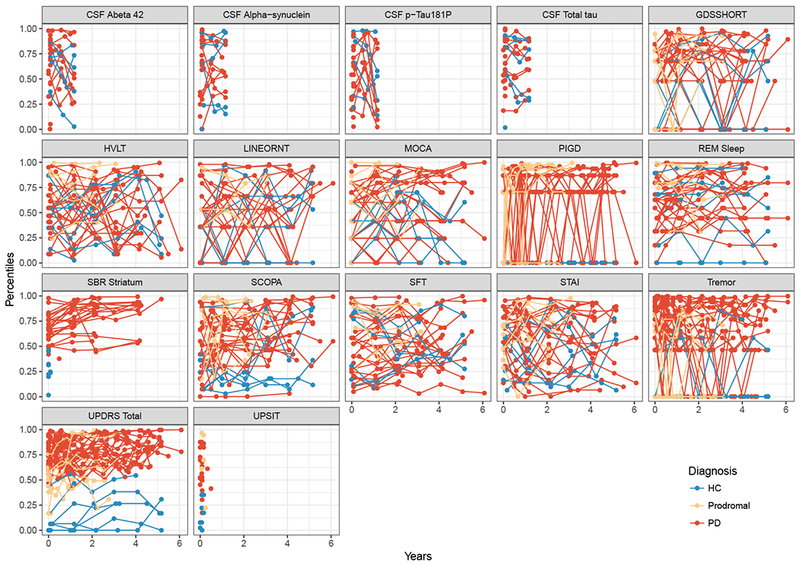
Observed subject-specific profile showing the profiles for 50 randomly selected subjects per out-come and by disease category.

Abbreviations: PIGD, Posture Instability and Gait Difficulty; RBD, REM sleep behavior disorder; UPSIT, University of Pennsylvania Smell Identification Test; MOCA, Montreal Cognitive Assessment; HVLT, Hopkins Verbal Learning Test; GDS, Geriatric Depression Scale; SFT, Semantic Fluency Test; SCOPA, Scale for Outcomes in Parkinson’s; LINEORT, Line Orientation Test; UPDRS, Unified Parkinson Disease Rating Scale; STAI, State Trait Anxiety Index; PD, Parkinson Disease; HC, Healthy Control.

4.2. Statistical Analysis

Figure 1a demonstrates that some of the outcomes more clearly distinguished between HC and PD than others. These measures were likely to carry more information related to latent time. Hence, our statistical analysis was limited to 8 of these outcomes namely, PIGD, SBR Striatum, SCOPA, Tremor, UPDRS, UPSIT, CSF synuclein and REM sleep behavior disorder. An analysis with all 17 outcomes is included in the Appendix.

We analyzed the data using the model described in Section 3 with three Markov chains, each run for 8000 iterations, including a warm-up of 4000 iterations, which is discarded. The LTJMM and the proposed LTJMM-H were implemented and the best model was selected according to two model selection criteria, the Widely Applicable Information Criterion (WAIC) and the Leave-One-Out Cross-validation Information Criterion (LOOIC). The LTJMM-H was chosen over the LTJMM since it produced lower WAIC and LOOIC values of 61054.8 and 62158.01 as compared to 61203.94 and 62290.43 for the homogeneous version, respectively. For the analysis of all 17 outcomes, WAIC and LOOIC for the LTJMM-H were 117860 and 120166.7, which was lower compared to the LTJMM values of 143431.9 and 145055.2, respectively.

Posterior means with corresponding 95% posterior credible intervals are reported in Table 4 for the selected model. Figure 3 shows the density plot of estimated random latent time shifts by diagnostic categories. Although diagnostic category was not included in the model, the model seemed to accurately reveal the temporal ordering of disease state consistent with the diagnosis groups and biology of PD. The distribution of latent time overlapped much more between HC and prodromal compared to HC and PD groups. This was not surprising since HC shared with both prodromal and PD some non-motor features (sleep disturbances, constipation, olfactory deficits, depression), but HC shared fewer features with PD than prodromal. Thus, the latent time shift estimates provided a continuous alternative to diagnosis, which was objectively derived from a comprehensive joint model of longitudinal measures of disease progression (Li et al., 2017). Comparing results from the two sets of outcomes, Table 4 and Table A.1 show that the model was generally robust to the inclusion of less informative outcome measures, but density plots, in Figure 3 and Figure A.1, show that latent time was more successful in parsing out the diagnosis groups when the less informative outcomes were omitted.

Table 4:

Results of posterior estimates of parameters and corresponding 95% credible interval for model with 8 outcomes from the Parkinson’s Progression Markers Initiative (PPMI).

Parameter	Posteri or Mean	95% Credible Interval	Parameter	Posteri or Mean	95% Credible Interval
CSF Alpha-synuclein			SCOPA
Intercept	0.8976	(0.4341,1.3793)	Intercept	−2.3726	(−2.7089,−2.0074)
Age	−0.0123	(−0.0200,−0.0050)	Age	0.0336	(0.0279,0.0387)
Female	−0.1160	(−0.2745,0.0401)	Female	0.5104	(0.3944,0.6296)
Latent time, γ1	0.0274	(0.0190,0.0363)	Latent time, γ5	0.0406	(0.0338,0.0486)
Error Variance, σ1	0.4288	(0.4023,0.4552)	Error Variance, σ5	0.4683	(0.4559,0.4819)
PIGD			Tremor
Intercept	−1.9367	(−2.6663,−1.1232)	Intercept	0.3527	(−0.3759,1.1549)
Age	0.0114	(−5e-04,0.0226)	Age	−0.0174	(−0.0295,−0.0064)
Female	0.0866	(−0.1579,0.3315)	Female	−0.1660	(−0.3967,0.0813)
Latent time, γ2	0.1415	(0.1225,0.1621)	Latent time, γ6	0.1236	(0.1084,0.1404)
Error Variance, σ2	1.1573	(1.1347,1.1788)	Error Variance, σ6	0.8108	(0.7962,0.827)
REM Sleep			UPDRS Total
Intercept	0.2397	(−0.1764,0.6504)	Intercept	−0.2535	(−0.6679,0.176)
Age	−0.0053	(−0.0118,8e-04)	Age	0.0059	(−8e-04,0.0123)
Female	−0.1052	(−0.2437,0.0494)	Female	−0.0364	(−0.1758,0.0979)
Latent time, γ3	0.0446	(0.0364,0.053)	Latent time, γ7	0.0880	(0.0769,0.0999)
Error Variance, σ3	0.5806	(0.5646,0.5968)	Error Variance, σ7	0.3494	(0.343,0.3559)
SBR Striatum			UPSIT
Intercept	−0.8843	(−1.2600,−0.5038)	Intercept	−1.2072	(−1.6254,−0.7688)
Age	0.0157	(0.0098,0.0215)	Age	0.0206	(0.0138,0.0275)
Female	−0.0677	(−0.2017,0.0604)	Female	−0.2175	(−0.348,−0.0731)
Latent time, γ4	0.0599	(0.0502,0.0697)	Latent time, γ8	0.0511	(0.0418,0.0615)
Error Variance, σ4	0.2118	(0.2002,0.2237)	Error Variance, σ8	0.3688	(0.0688,0.6602)
Heterogeneous parameters			Model criteria
τ1	5.1320	(4.4178,5.8806)	WAIC	61054.80
τ2	−0.0071	(−.018,0.0033)	LOOIC	62158.01
τ3	−0.0184	(−0.2247,0.1919)

Figure 3:

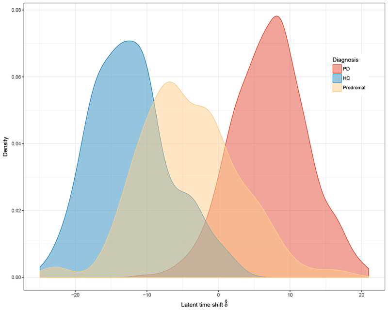
Distribution of estimate of time shift, ${\widehat{\delta }}_{\iota }$ by disease status.

Abbreviations: PD, Parkinson’s Disease; HC, Healthy Control.

Figure 4 (and Figure A.2 for all outcomes) shows the correlation of random slopes between pairs of outcomes. Consistent with the observed correlation matrix in Figure 1b, we observed that the slopes for PIGD were correlated with UPDRS Total. Similarly, GDSSHORT and STAI showed moderate association. In general, we observed that the biological markers shared a stronger association amongst markers compared to their association with clinical markers.

Figure 4:

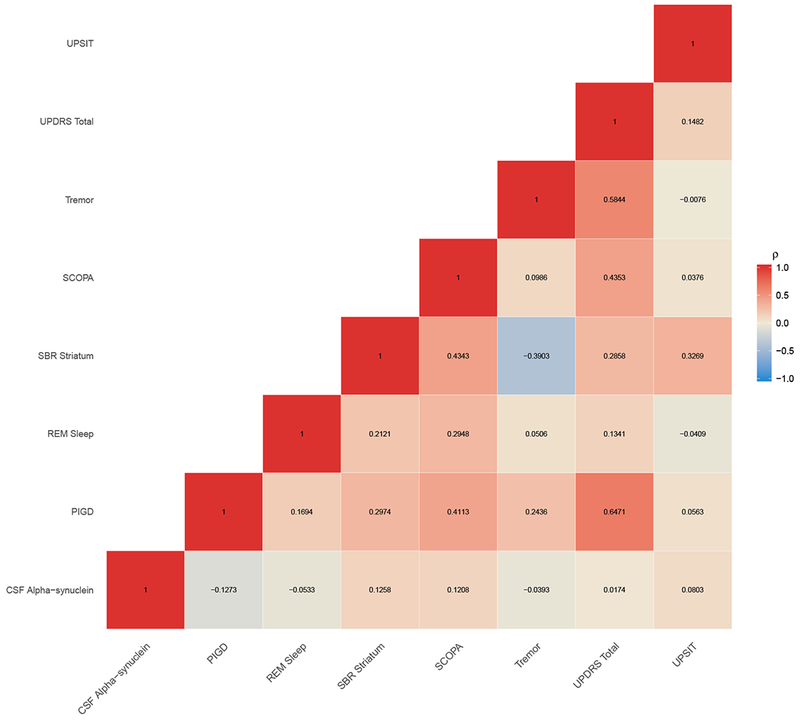
Correlation between random slopes for pair of outcomes.

Abbreviations: PIGD, Posture Instability and Gait Difficulty; RBD, REM sleep behavior disorder; UPSIT, University of Pennsylvania Smell Identification Test; SCOPA, Scale for Outcomes in Parkinson’s; UPDRS, Unified Parkinson Disease Rating Scale; PD, Parkinson Disease; HC, Healthy Control.

Figure 5 shows the subject-level predicted severity versus age for ten randomly selected participants. The model reasonably predicted the trend and direction of individual trajectories albeit with some variation. For subjects with more time points, the predicted trajectories appeared to perform better, with some reduction in the difference between the observed and predicted trajectories compared to subjects with fewer time points. Placed side-by-side in Figure 6a and b are the observed and predicted subject-level trajectories against age. The two sets of trajectories appeared similar giving an indication that the model was predicting reasonably well. In addition, SBR striatum and Total UPDRS in Figure 6a and b clearly showed the discriminability of these measures between disease stages in the observed and predicted trajectories.

Figure 5:

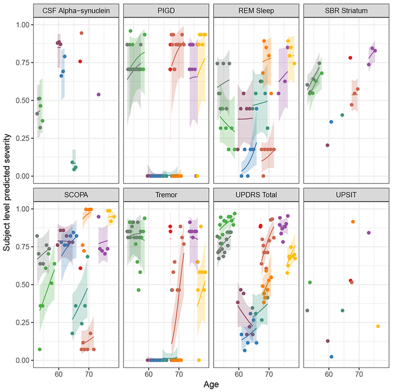
Subject-level prediction for random subjects. Each color represents the predicted profile of a randomly selected individual.

Abbreviations: PIGD, Posture Instability and Gait Difficulty; REM Sleep, Rapid Eye Movement Sleep behavior disorder; UPSIT, University of Pennsylvania Smell Identification Test; SCOPA, Scale for Outcomes in Parkinson’s; UPDRS, Unified Parkinson Disease Rating Scale; PD, Parkinson Disease; HC, Healthy Control.

Figure 6:

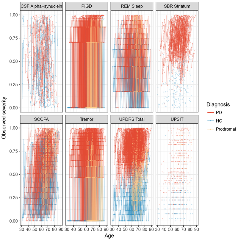
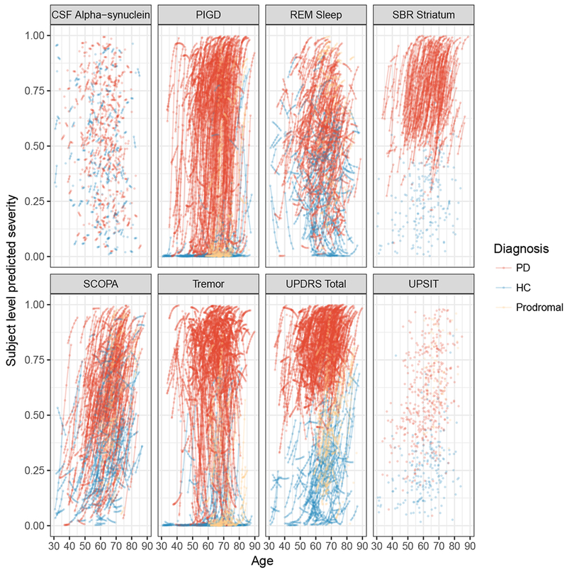
(a) Observed severity

(b) Subject-level predicted severity

The left panel shows observed trajectories. The right panel shows the predicted profile for all subjects by outcome.

Abbreviations: PIGD, Posture Instability and Gait Difficulty; REM Sleep, Rapid Eye Movement Sleep behavior disorder; UPSIT, University of Pennsylvania Smell Identification Test; SCOPA, Scale for Outcomes in Parkinson’s; UPDRS, Unified Parkinson Disease Rating Scale; PD, Parkinson Disease; HC, Healthy Control.

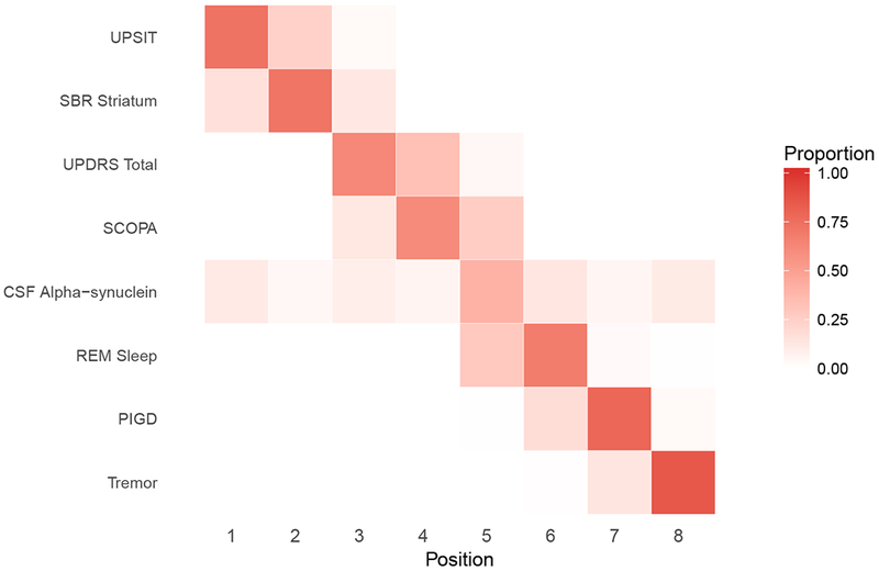
Figures 7 displays the average long-term population trajectories for females with progressive disease. To generate these plots, it was necessary to “calibrate” the independent variables age and latent time by assigning the latent time for any given age. For the purposes of these plots, we assumed the estimated median latent time among HCs (−13 years) at the average age for the entire sample (61 years). This figure indicates that PIGD and tremor reached the 50th percentile later in the disease progression compared to UPDRS, which occurred much earlier. We also fitted the model treating the UPDRS subtests I, II and III as separate outcomes (see supplemental material, Figure A.3b). We found that UPDRS I (mental) reached the 50th percentile level first on average, followed by UPDRS III (motor) and II (activities of daily living) in close succession. Due to the strong gender effect, as can be observed from the table of estimates, a similar plot for males will position SCOPA differently in the ordering (see Figure 8).

Figure 7:

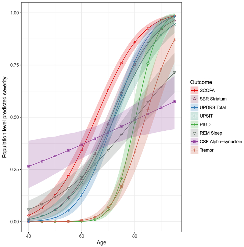
Population level predicted severity for female with mean age and median latent time of a healthy control. The legend is ordered by the age at which the predicted severity level for each outcome is 0.5 (sliced horizontally).

Abbreviations: PIGD, Posture Instability and Gait Difficulty; REM Sleep, Rapid Eye Movement Sleep behavior disorder; UPSIT, University of Pennsylvania Smell Identification Test; SCOPA, Scale for Outcomes in Parkinson’s; UPDRS, Unified Parkinson Disease Rating.

Figure 8:

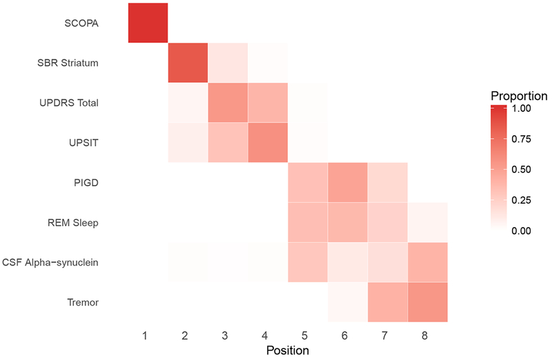
(a) Female.

(b) Male.

Positional variance diagram of the central ordering. The x-axis is the event position. Difference in ordering may be attributed to the strong effect of gender on some of these outcomes.

Abbreviations: PIGD, Posture Instability and Gait Difficulty; REM Sleep, Rapid Eye Movement Sleep behavior disorder; UPSIT, University of Pennsylvania Smell Identification Test; SCOPA, Scale for Outcomes in Parkinson’s; UPDRS, Unified Parkinson Disease Rating Scale; PD, Parkinson Disease; HC, Healthy Control.

Figure 8, a “positional variance diagram”, shows the estimated variation in the ordering of marker abnormalities for female and males. Figure 8 was derived by slicing Figure 7 horizontally at the 50th percentile and observing the order of markers as they appear from left to right. We used the posterior distribution to evaluate the uncertainty in these estimated orderings. For each draw from the posterior distribution, we generated curves similar to Figure 7 and sliced horizontally at the 50th percentile to determine the ordering of marker abnormalities for that posterior sample. The diagram represents the distribution (proportion of MCMC samples) of the outcome orderings. The bolder the color of the cell, the higher the certainty of the ordering for that outcome. In Figure 9, we display the positional diagram based on subject-level predictions. For each subject in the sample, we ordered the outcomes based on the age the 50th percentile of the outcome is attained. As one might expect, there was greater variation in the orderings from subject-to-subject (Figure 9) compared to the average ordering for the sample (Figure 8)

Figure 9:

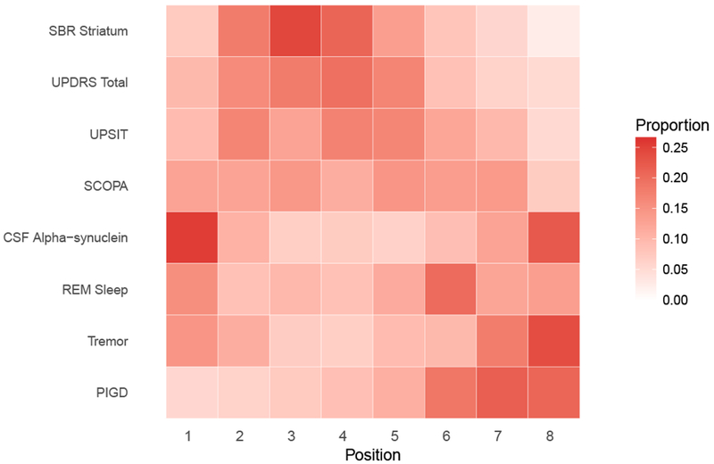
Positional variance diagram of the central ordering.

Abbreviations: PIGD, Posture Instability and Gait Difficulty; REM Sleep, Rapid Eye Movement Sleep behavior disorder; UPSIT, University of Pennsylvania Smell Identification Test; SCOPA, Scale for Outcomes in Parkinson’s; UPDRS, Unified Parkinson Disease Rating Scale; PD, Parkinson Disease; HC, Healthy Control.

5. Discussion

In this paper, we applied a joint mixed effect model with latent time to analyze the various stages of PD included in the PPMI study. We found that although diagnostic category was not included in the model, it seems to accurately reveal the temporal ordering of disease state consistent with diagnosis categorization at baseline. In other words, the distribution of the estimates of the latent time reflected the subjective assessment of patient disease status at baseline.

In addition, the association between estimated random-effects revealed that biological markers share stronger pair-wise association but a weaker association with clinical markers. The biomarkers not being very informative (greater variance and lower signal-to-noise) probably explains this weak association with clinical outcomes. It is worth mentioning that, the role of γ-amyloid and tau protein as biomarkers in PD is not well established, but a number of publications report altered CSF Aβ1-42, t-tau or p-tau in patients with PD with or with-out dementia compared with HC (Brockmann et al., 2015). Clinical markers also tend to be correlated among each other. Posture Instability and Gait Difficulty (PIGD) and Total Unified Parkinson Disease Rating Scale (UPDRS), and Geriatric Depression Scale (GDSS) and State Trait Anxiety Index (STAI) sharing strong to moderate associations. Inspection of observed and predicted severity shows that SBR striatum and Total UPDRS can provide better discrimination between disease stages.

Long-term population level trajectories were also derived from the proposed model. The results indicated late manifestation of PIGD and tremor but earlier Total Scale for Outcomes in Parkinson’s (SCOPA) and Total UPDRS abnormalities. The SCOPA and UPDRS include non-motor features that appear at prodromal disease stages (earlier in the course of the illness). The positional variance diagram provided an ordering consistent with that from the population trajectories. Similar trajectories can be obtained for any sub-group of the population with ease using our modeling approach. It should be kept in mind that the data used to develop the models are restricted to short-term follow-up after enrollment (median < 4 years), which might limit predictive accuracy when evaluated over longer periods of disease progression.

We also demonstrated through a limited simulation study that allowing heterogeneity in the variance of latent time can improve LTJMM fit. The variance of the latent time was modeled in terms of observed baseline covariates. Particularly, the simulation indicated that estimation of parameters is consistent with the LTJMM model except that the between-subject latent time variance is severely biased. Given the importance of the subject-specific latent time as a data-driven alternative to categorical disease status, it is critical that the latent-time variance is accurately estimated. Violation of the homogeneous latent time can, therefore, be detrimental. We encourage the exploration of different sub-models to determine which baseline covariates are significant in explaining the between-subject latent time variation. In the application of the two models to the PPMI study, both WAIC and LOOIC favored the extended LTJMM model with heterogeneous latent time.

References

- 1.Brockmann K, Schulte C, Deuschle C, Hauser A-K, Heger T, Gasser T, Maetzler W, & Berg D (2015). Neurodegenerative CSF markers in genetic and sporadic PD: Classification and prediction in a longitudinal study. Parkinsonism and Related Disorders, 21, 1427–1434. [DOI] [PubMed] [Google Scholar]
- 2.Guerrero R, Schmidt-Richbergh A, Ledig C, Tong T, Wolz R, & Rueckert D (2016). Instantiated mixed effects modeling of Alzheimer’s disease markers. NeuroImage, 142, 113–125. [DOI] [PubMed] [Google Scholar]
- 3.Iddi S, & Molenberghs G (2012). A joint marginalized multilevel model for longitudinal outcomes. Journal of Applied Statistics, 39,24132430. [Google Scholar]
- 4.Kennedy RE, Cutter GR, Wang G, & Schneider LS (2015). Using baseline cognitive severity for enriching Alzheimer’s disease clinical trials: How does mini-mental state examination predict rate of change? Alzheimer’s & Dementia: Translational Research & Clinical Interventions, 1,46–52. [DOI] [PMC free article] [PubMed] [Google Scholar]
- 5.Klotsche J, Reese JP, Winter Y, Oertel WH, Irving H, Wittchen H, Rehm J, & Dodel R (2011). Trajectory classes of decline in health-related quality of life in Parkinson’s disease: A pilot study. Value in Health, 14,329–338. [DOI] [PubMed] [Google Scholar]
- 6.Lewandowski D, Kurowicka D, & Joe H (2009). Generating random correlation matrices based on vines and extended onion method. Journal of Multivariate Analysis, 100, 1989–2001. [Google Scholar]
- 7.Li D, Iddi S, Thompson WK, & Donohue MC (2017). Bayesian latent time joint mixed effect models for multicohort longitudinal data. Statistical Methods in Medical Research, 0,00–00. doi: 10.1177/0962280217737566. [DOI] [PubMed] [Google Scholar]
- 8.Luo S (2014). A Bayesian approach to joint analysis of multivariate longitudinal data and parametric accelerated failure time. Statistics in Medicine, 33, 580–594. [DOI] [PMC free article] [PubMed] [Google Scholar]
- 9.Luo S, & He B (2016). Joint modeling of multivariate longitudinal measurements and survival data with applications to Parkinson’s disease. Stat Methods Med Res, 25, 1346–1358. [DOI] [PMC free article] [PubMed] [Google Scholar]
- 10.Sturkenboom IHWM, Graff MJL, Hendriks JCM, Veenhuizen Y, Munneke M, Bloem BR, & Sanden MWN (2014). Efficacy of occupational therapy for patients with Parkinson’s disease: a randomized controlled trial. The Lancet Neurology, 13,557–566. [DOI] [PubMed] [Google Scholar]
- 11.Tsiatis AA, & Davidian M (2004). A joint modeling of longitudinal and time-to-event data: An overview. Statistica Sinica, 14, 809–834. [Google Scholar]
Associated Data
This section collects any data citations, data availability statements, or supplementary materials included in this article.