Studying Structural Dynamics of Potassium Channels by Single-Molecule FRET

Abstract

Single-molecule FRET (smFRET) can visualize conformational dynamics of individual ion channels in lipid bilayers of defined composition. Dynamic and distance measurements from smFRET, combined with single channel recordings, can provide previously unattainable direct mechanistic insights into ion channel function and modulation. smFRET measurements require site-specific fluorophore labeling between two distinct sites, which is a major challenge for multimeric ion channels. This chapter aims to provide a step-by-step protocol: (1) to design concatemeric constructs with only two cysteine residues within a homotetrameric channel; (2) to express, purify, label, and reconstitute channel proteins; (3) to perform smFRET imaging on channel proteins in liposomes with an objective-based Total Internal Reflection (TIRF) microscope; and finally (4) to analyze the FRET distributions and dynamics that reflect the dynamic conformational transitions of ion channels in membranes.

1. Introduction

Ion channels are integral membrane proteins that selectively conduct ions, thereby controlling many physiological processes [1]. Since gated currents through single-ion channel pores were first observed, over 40 years ago [2], many channels have been recorded and analyzed at the single-channel current level, revealing mechanistic insights to the physical states underlying gating transitions [3]. Over the last 20 years, high-resolution structures of ion channels in different static conformations have informed the structural changes of the gating transitions [4–8]. However, the atomic structures obtained by crystallography or electron-microscopy are typically from protein molecules frozen in stable states and often in environments other than lipid bilayers. Reconstructing the conformational trajectories from these static ‘snapshots’ and correlating them with dynamic gating events of ion channels in cell membranes may not always be straightforward, or even apparent.

Fluorescent resonant energy transfer (FRET) can be used to assess intramolecular structures and structural changes in response to physical or chemical stimuli. Single-molecule FRET (smFRET) can report unsynchronized conformational trajectories, reveal structural distributions and transitions, and uncover rare structural states, which are unattainable for ensemble measurements [9, 10]. In recent years, smFRET has been extensively used to examine conformational dynamics of nucleic acids and soluble proteins, but has rarely been applied to membrane proteins [11–15]. Studying ion channels, in particular multimeric ion channels, with smFRET presents significant technical challenges of protein purification, fluorophore labeling, and functional reconstitution.

In this chapter, we provide step-by-step protocols detailing how to prepare smFRET samples for the study of structural dynamics of tetrameric potassium channels. We describe critical controls to help avoid potential artifacts and bias in such measurements. The protocols we describe may also be useful for studying conformational dynamics of other ion channels or transmembrane proteins.

2. Materials

Prepare all the solutions using ultrapure Milli-Q water (resistance >18.2 MΩ). All the chemicals should be of analytic grade purity, except as specified.

2.1. Plasmids and Proteins

KirBac1.1 plasmids, as well as the cysteine configurations of the resulting tetrameric proteins, as shown in Fig. 1, are described in detail in original publications [15, 16], and are available upon request (see Note 1).

Fig. 1.

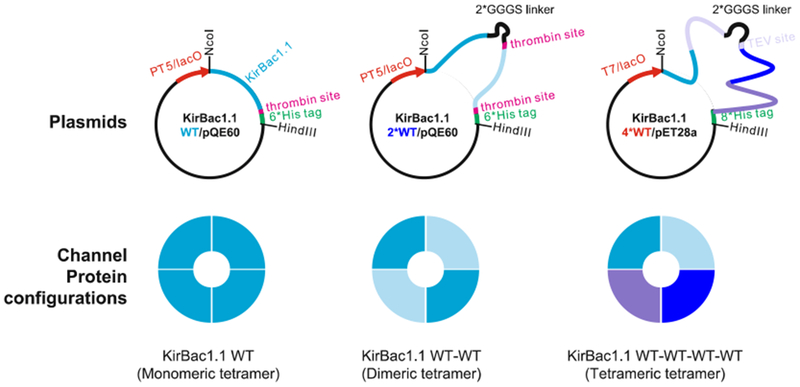
KirBac1.1 plasmids and the subunit configurations of the resulting proteins for smFRET studies (Wang et al. [15])

2.2. Protein Purification and Fluorophore Labeling

1. Cell Resuspension Buffer (CSB): 50 mM Tris–HCl, 150 mM KCl, 250 mM Surcose, 10 mM MgCl₂, 10 mM imidazole, pH 8.0, containing 2 mM TCEP, 0.02 mg/mL DNase I, 1 EDTA-free Protease Inhibitor Cocktail tablet per 50 mL resuspension (see Note 3).

2. Washing Buffer (WB): 50 mM Tris–HCl, 150 mM KCl, 5 mM n-Decyl-β-d-Maltopyranoside (DM), 10 mM imidazole, 2 mM TCEP, pH 8.0.

3. Elution Buffer (EB): 50 mM Tris–HCl, 150 mM KCl, 5 mM DM, 400 mM imidazole, 2 mM TCEP, pH 8.0.

4. Labeling Reaction Buffer (LRB): 20 mM Hepes-KOH, 150 mM KCl, 5 mM DM, pH 7.0 (see Note 4).

5. Gel Filtration Buffer (GFB): 20 mM Hepes-KOH, 150 mM KCl, 5 mM DM, 1 mM TCEP pH 7.5.

2.3. Protein Reconstitution

1. POPE/POPG lipid solution: POPE/POPG/biotinylated-POPE lipid mixer (73:25:2, w/w/w), dissolved in 20 mM Hepes-KOH, 150 mM KCl, 30 mM CHAPS, pH 7.5, with final total lipid concentration as 10 mg/mL (see Note 5).

2. Reconstitution Buffer (RB): 20 mM Hepes-KOH, 150 mM KCl, pH 7.5.

2.4. PEG/Biotin-PEG Passivation

1. Dremel-3000 with 0.75 mm diamond drill bit.

2. Slides (25 × 75 mm) and coverslips (24 × 60 mm).

3. Glass-staining dishes and 250 mL flask.

4. Propane torch.

5. Nitrogen gas.

6. Methanol.

7. Acetone.

8. 3.0 M KOH.

9. Acetic acid, glacial.

10. N-(2-Aminoethyl)-3-Aminopropyltrimethoxysilane.

11. mPEG-Succinimidyl Carbonate, MW5000.

12. Biotin-PEG-SC-5000.

13. 0.1 M sodium bicarbonate.

2.5. Single-Molecule Imaging

1. Saturated 6-hydroxy-2,5,7,8-tetramethylchroman-2-carboxylic acid (Trolox) solution: Dissolve 30 mg of Trolox in 10 mL of milliQ water, mix gently overnight on a rocker, then pass through a syringe filter with 0.22 μm pore size, the final concentration is ~3.0 mM.

2. Oxygen scavenging stock (Gloxy, 100×): 1 mg/mL (~160 U/mL) glucose oxidase, and 0.04 mg/mL (~2200 U/mL) catalase in 50 mM Tris–HCl, 50 mM NaCl, pH 8.0. The stock can be stored at −20 °C for up to 6 months.

3. NBA stock (100×): 200 mM NBA (4-nitrobenzyl alcohol) dissolved in DMSO, store at −20 °C.

4. COT stock (100×): 200 mM COT (cyclooctatetraene) dissolved in DMSO, store at −20 °C.

5. Imaging buffer: 20 mM Hepes-KOH, 150 mM KCl, 1 mM EDTA, 1 mM EGTA, pH 7.5, containing 0.8% dextrose, ~3 mM Trolox, degassed by a low vacuum pump for 10 min (see Note 6).

6. T50: 10 mM Tris–HCl, 50 mM NaCl, pH 8.0.

7. Crimson fluorescent beads (ThermoFisher, CATA#F8806, 0.2 um size with excitation and emission peak at 625 and 645 nm, respectively).

2.6. Customized TIRF Microscope and Software

1. The configuration of the TIRF microscope with a dual-view beam splitter is illustrated schematically in Fig. 2. The customized objective-based TIRF microscope we used was constructed on a Nikon TE-2000S inverted fluorescence microscope with a 100× 1.49NA Nikon Apo TIRF objective lens. The imaging system is equipped with a Nikon D-Eclipse Cl TIRF illumination system containing a 532 nm (Sapphire 532-LP, 100 mW, Coherent Inc.) and a 640 nm (OBIS 640-LX, 40 mW) laser. A CRISP autofocus system (780 nm, ASI Inc.) is used to compensate for focus drift due to thermal fluctuations or mechanical vibrations that are not avoided by the use of a floating air table. An OptoSplit II LS Image Splitter (Cairn Research Inc) with ZT638RDC-UF2/ET585/65/ET700/75 filter set (Chroma Inc.) is used to split the donor and acceptor emissions, which are imaged by an Evolve 512 delta emCCD camera (Photometries Inc.).

2. NIS-element AR software is used for collecting images and movies (see Note 6).

3. IDL8.2 software is used to analyze single-molecule image movies. A set of IDL scripts developed by the group of Dr. Taekjip Ha to align donor and acceptor channels, identify individual molecules, and extract the fluorescence intensity time traces is available for download at https://cplc.illinois.edu/software/.

4. Matlab is used to visualize, select, and analyze these traces interactively. A script set developed by the Ha group is available for download at https://cplc.illinois.edu/software/.

Fig. 2.

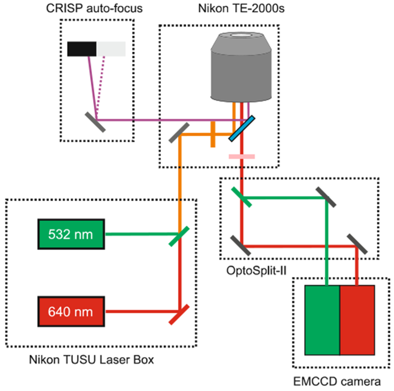
Schematic of the optical configuration of the TIRF microscope for single-molecule FRET imaging

3. Methods

3.1. Protein Purification and Labeling

Perform protein purification and labeling procedures by following the flowchart in Fig. 3, with additional details included in the following protocols.

Fig. 3.

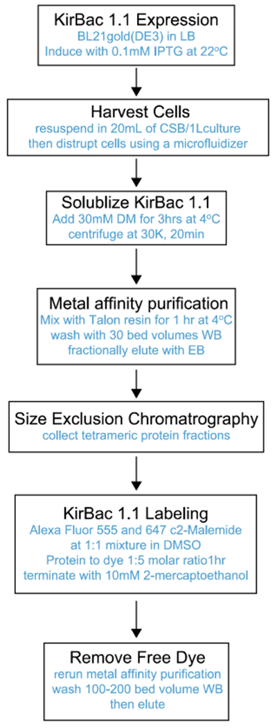
Flowchart of protein expression, purification, and fluorophore labeling

1. Protein expression and purification.

   • (a)Transform KirBac1.1 cysteine mutant constructs into the E. coli BL21 gold(DE3) host strain, inoculate the transformants in Luria Broth medium, grow at 37 °C until OD600 reaches ~0.6, then induce with 0.1 mM IPTG at 22 °C overnight.
   • (b)Harvest E. coli expressing KirBac1.1 proteins by centrifugation and then resuspend the cells in CSB, 20 mL/L of culture.
   • (c)Break cells by passing through an M-110P Microfluidizer 3×, with an operating pressure of 18,000 psi, cooling with an ice/water mixture.
   • (d)Extract KirBac1.1 proteins by adding 30 mM DM and rotate at 4 °C for 3 h.
   • (e)Spin the cell lysate at 30,000 × g for 20 min, mix the supernatant with Talon metal affinity resin (0.4 mL 50% slurry per liter of culture), and gently stir in a rocker for 1 h at 4 °C.
   • (f)Spin down the resin at 300 × g, discard the supernatant and pour the resin into a small column, wash with 30 bed volumes of WB.
   • (g)Elute the KirBac1.1 proteins with EB (see Note 7).

2. Protein labeling.

   • (a)Perform size-exclusion chromatography (SEC) on the purified protein using a Superdex-200 10/300 column with a flow rate of 0.5 mL/min, collecting 0.5 mL fractions with an AKTA FPLC system. Use LRB as running buffer, collect the KirBac1.1 tetrameric protein fractions, with peak usually at ~12.0 mL, and then concentrate to 2 mg/mL with an Amicon Ultra-4 centrifugal filter (see Note 8).
   • (b)Start the fluorophore labeling immediately by adding DMSO-dissolved Alexa Fluor 555 and 647 c2 maleimide (1:1 mixture) to the KirBac1.1 protein solution to a final protein:dye molar ratio of 1:5. Conduct the labeling reaction at room temperature for 1 h, then terminate with 10 mM 2-mercaptoethanol (see Note 9).
   • (c)Separate the KirBac1.1 protein conjugated with fluorophores by conducting another metal affinity chromatographic purification as described in step 1e–g (see Note 10).

3.2. Protein Reconstitution

1. Add 10 μg KirBac1.1 protein to 200 μL of POPE/POPG lipid solution (10 mg/mL) to make a final protein:lipid ratio of 1:200 (w/w), and then incubate at room temperature for 20 min.

2. Prepare a Sephadex G-50 column with 2 mL bed volume, equilibrate it with RB, and then centrifuge for 30 s in a swinging bucket centrifuge at 1000 × g to dry the column.

3. Load 200 μL lipid-KirBac1.1 protein mixture onto the spin-dried column and then collect KirBac1.1 proteoliposomes by centrifuging at 800 × g for 30 s.

4. Immediately before single-molecule imaging experiments, extrude the proteoliposomes 29 times through a polycarbonate membrane with a pore size of 50 nm (see Note 11).

3.3. Single-Molecule Imaging

1. Prepare sample chamber slide for single-molecule imaging as summarized in the flowchart in Fig. 4.

   • (a)Drill a pair of 0.75 mm diameter holes in the glass slide to form each sample chamber; up to five separate sample chambers can be made for each slide of regular size (1 × 3 in.).
   • (b)Sonicate the glass slide and coverslips in a glass-staining dish for 30 min in acetone, 30 min in methanol, 30 min in 3 M KOH, rinsing with milliQ water between each solution.
   • (c)Rinse the slides and coverslips 6× with MilliQ water.
   • (d)Rinse 3× with methanol and then dry the slides and coverslips with nitrogen gas.
   • (e)Flame slides (<20 s) and coverslips (<3 s) to remove any fluorescent organic molecules and set aside in clean staining jars.
   • (f)Clean a flask by filling with methanol and sonicating for 5 min, then rinse 3× with methanol.
   • (g)Add 100 mL methanol to the clean flask, then add 5 mL acetic acid and 1 mL amino-silane using a glass pipette. Mix the solution by gently shaking, then add it into staining jars containing clean glass slides and coverslips, incubate for 10 min, sonicate for 1 min, and then incubate for another 10 min.
   • (h)Wash the mixture off by rinsing with methanol six times and dry the slides and coverslips using nitrogen gas.
   • (i)For ten sample chambers, dissolve 100 mg mPEG and 3 mg biotin-PEG in 800 μL 0.1 M sodium bicarbonate (freshly made and filtered through a 0.22 μm filter). Mix with a pipette gently and then spin at 14,000 × g for 1 min.
   • (j)Apply 70 μL PEG mixture on each slide, place coverslip over each slide, and then incubate in a dark and humid box for 4 h or overnight.
   • (k)Dissemble the slides and coverslips, wash with MilliQ water extensively, then dry with nitrogen gas.
   • (l)Put each slide/coverslip set in a 50 mL falcon tube with coated surfaces away from each other, seal the tube in a vacuum bag with a regular food saver and then store at −20 °C.
   • (m)Before smFRET imaging experiments, assemble the slides and coverslip using double-sided tape (~0.1 mm thick) and seal the chamber using instant Epoxy.
   • (n)A complete video instruction is also available at Journal of Visualized Experiments, demonstrated by Chandradoss et al. [17] (http://www.jove.com/video/50549/surface-passivation-for-single-molecule-protein-studies).

2. Alignment of the OptoSplit II LS Image Splitter.

   • (a)Prepare a bead slide for aligning the OptoSplit II LS Image Splitter by diluting the crimson fluorescent beads (Invitrogen, Cata#F8806) 50× with 1 M Tris-HCl, pH 8.0. Assemble a clean coverslip and slide with double-sided tape (~0.1 mm thick), add and then seal the diluted beads into the slide chamber by instant Epoxy.
   • (b)Add a drop of immersion oil to the objective lens and mount the bead slide on the microscope with the coverslip facing the objective lens. Ensure there are no visible air bubbles trapped between the coverslip and the objective lens.
   • (c)Excite the crimson fluorescent beads with a 532 nm laser, adjust the laser incident angle to set the evanescent field penetration depth, to ensure that only the crimson fluorescent beads on the inner surface of the coverslip are excited.
   • (d)Adjust the OptoSplit II LS Image Splitter, align the donor (from 545 to 620 nm) and acceptor (from 660 and 750 nm) channels to the left (X[1–256]:Y[1–512]) and right half (X[257–512]:Y[1–512]) of the emCCD camera chip, respectively. In live-acquisition mode, visually inspect the alignment of the donor and acceptor channels pixel by pixel, then acquire a short movie and analyze the mapping with the IDL scripts. Iteratively repeat alignment and mapping until fluorescence emissions from the same beads appear at equivalent positions of the donor and acceptor channels with deviations less than 2 pixels for both horizontal and vertical directions.

3. Collect movies on the proteoliposomes.

   • (a)Remove the aligning slide and mount a sample chamber on the microscope.
   • (b)Hydrate the sample chamber with 50 μL of T50, incubate for ~1–5 min.
   • (c)Set the exposure time, focus on the inner surface of the coverslip by looking for fluorescent contaminates or surface scratches, then adjust the laser power, incident angle, and the electronic multiplying (EM) gain to optimize image quality.
   • (d)Add 50 μL of neutravidin solution (0.25 mg/mL, in T50), incubate for ~1–5 min.
   • (e)Dilute KirBac1.1 proteoliposomes with reconstitution buffer, starting at 1:100,000 dilution, and load the mixture into the slide chamber. The liposomes will immobilize on the surface of the coverslip as illustrated schematically in Fig. 5. Increase the proteoliposome concentration to optimize the number of emission spots in each view, but well separated from each other (see Note 12).
   • (f)Take 100 μL of imaging buffer, add 1 μL COT and 1 μL NBA, then add 1 μL Gloxy and gently mix the imaging buffer with a pipette, flush away the proteoliposome samples with imaging buffer, and collect 5–10 movies for every sample/condition (see Note 13).

Fig. 4.

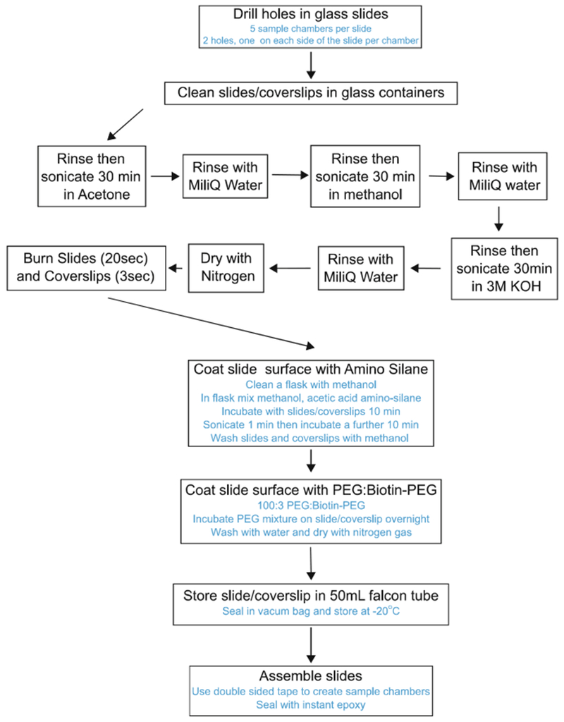
Flowchart of protocol for preparing slide chamber for single-molecule imaging

Fig. 5.

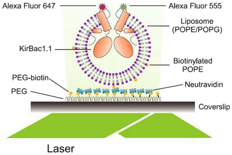
Objective-based TIRF setup to perform single-molecule imaging on KirBacl.1 reconstituted into liposomes

3.4. Data Analysis

3.4.1. Data Collection

The overall procedures to collect and analyze imaging data are summarized as a flowchart in Fig. 6. Identify single-molecule spots and extract time intensity profiles using the IDL script set. If the movies are collected by NIS-elements or μManager, export them first as .tif stack files and then convert them into .pma (8-bit binary image stack file format) files, using a Labview script developed in the Nichols lab, available upon request.

Fig. 6.

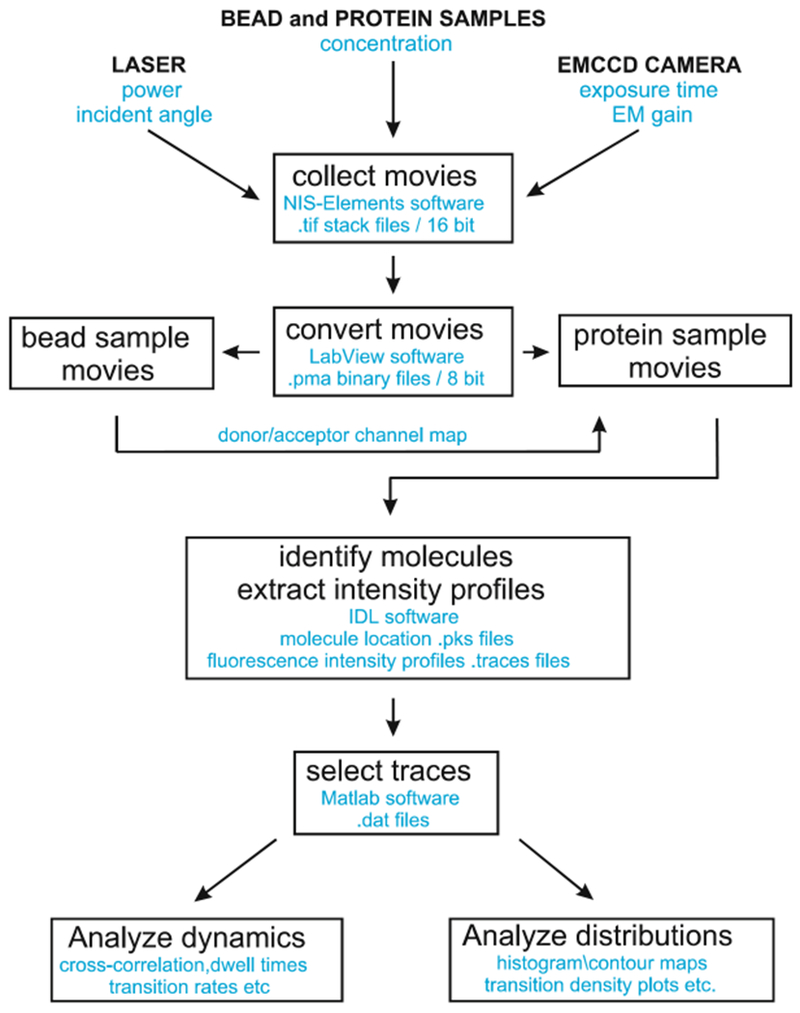
Flowchart for collection and analysis of smFRET data

3.4.2. Trace Selection

Visualize and manually select the traces using the Matlab script developed by the Ha group, then save them as .dat files, with time, donor, and acceptor intensities in three columns separated by a space. A good practice is to select traces independently by two researchers, at least for part of data, to ensure there is no significant bias in trace selection. The general standards to pick traces are (Fig. 7a, b):

1. Both donor and acceptor bleach in single steps.

2. The lifetime of the acceptor fluorophore is longer than 5 s.

3. The donor and acceptor intensity traces exhibit a clearly anti-correlated pattern.

4. There is no large variance (usually <20%) in total fluorescence intensities (i.e., the sum of the donor and acceptor fluorescence intensities).

5. The donor or acceptor should not have highly frequent or long-duration blinking events.

Fig. 7.

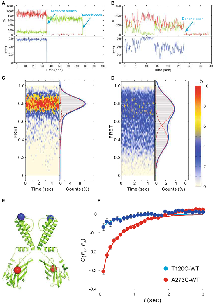
Studying structural dynamics of KirBac1.1 reconstituted into liposomes by single-molecule FRET, (a, b) Representative traces from dimeric KirBac1.1, with fluorophore labeling at the T120C and A273C sites, (c, d) FRET contour maps (left) and histograms (right) from KirBac1.1 with fluorophore labeling at the T120C and A273 sites, (e) Cartoon showing the KirBac1.1 crystal structure with T120 (blue) and A273 (red) labeling sites highlighted as spheres, (f) Cross-correlation analysis of the FRET signals at T120C sites (close to the selectivity filter) and at the A273C sites (in the cytoplasmic domain)

3.4.3. Calculate and Correct the FRET Efficiency

1. FRET efficiency is calculated by the following equation:

   $$E=\frac{F_{\mathrm{A}}-l\times F_{\mathrm{D}}}{F_{\mathrm{A}}-(F_{\mathrm{D}}\times l)+\gamma \times F_{\mathrm{D}}},$$

   where F_A and F_D are fluorescence intensities of the same molecule in the acceptor and donor channels; l is the leakage of the donor fluorescence into the acceptor channel, measured with the samples labeled with donor fluorophore only, on the same TIRF microscope with identical optical elements; γ is the gamma factor resulting from the difference in quantum yields and detection efficiencies between donor and acceptor fluorescence.
2. γ can be calculated by the following equation:

   $$\gamma =\frac{{F_{\mathrm{A}}}^{\mathrm{b}}-{F_{\mathrm{A}}}^{\mathrm{a}}}{{F_{\mathrm{D}}}^{\mathrm{a}}-{F_{\mathrm{D}}}^{\mathrm{b}}},$$

   where F_A^a, F_A^b, F_D^a and F_D^b are the fluorescence intensities of the same molecule in the acceptor (A) and donor channels (D) before (b) and after (a) acceptor photobleaching (see Note 14).

3.4.4. Analysis of FRET Signal Distributions

Contour maps and histograms are informative graphical representations of the data. Contour maps (Fig. 7c, d, left panels) show the averaged FRET signals over (in this case) the first 3 or 5 s of all recordings under a given condition and give a visual illustration of the time stability of the FRET signal, and the major FRET levels observed. Fitting the distributions (averaged FRET amplitude over the time segment) with a sum of Gaussian distributions implies discrete amplitudes, reflecting occupancy of distinct physical states with specific discrete distances between the fluorophores.

1. Mean FRET histograms can be calculated as the average of FRET histograms from each trace, after pooling all trace data from the same group (Fig. 7c, d).

2. To calculate the FRET contour map, extract the first 3 or 5 s of FRET data of each trace and calculate a histogram from each time point, then plot the contour map with X axis as time, Υ axis as FRET, and Z as relative counts, displayed using a customized color map (Fig. 7c, d).

3.4.5. Analysis of FRET Dynamics

Akin to single-ion channel analyses [1] lifetime distributions in discrete states can theoretically be assessed from smFRET traces. However, in practice, multiple FRET states without clearly defined amplitudes have precluded such an analysis of KirBac1.1. For FRET traces without discernable discrete states, dynamics can be quantitatively evaluated by performing autocorrelation analysis on FRET. If the trace data are very noisy, cross-correlation analysis between donor and acceptor fluorescence intensities can be performed. Such an analysis can still be used to infer dynamic flexibility between sites to which the specific fluorophore pair is attached. For instance, there is significant flexibility at residue A273C, reflected in a significant cross-correlation between fluorophore signals, but very little flexibility at residue T120C (Fig. 7e).

1. The autocorrelation of FRET can be analyzed by the following equation:

   $$C_{\text{auto}}(t)=\frac{\langle \Delta {\mathrm{FRET}}_0\times \Delta {\mathrm{FRET}}_t\rangle }{\langle \Delta {\mathrm{FRET}}_0^2\rangle },$$

   where ΔFRET₀ and ΔFRET_t are the variance of FRET at times 0 and t, respectively.
2. The cross-correlation of donor and acceptor fluorescence intensities can be analyzed with the following equation:

   $$C_{\text{cross}}(t)=\frac{\langle \Delta F_{\mathrm{D}}^0\times \Delta F_{\mathrm{A}}^t\rangle }{\langle \Delta F_{\mathrm{D}}^0\times \Delta F_{\mathrm{A}}^0\rangle },$$

   where $\Delta F_{\mathrm{D}}^0$, $\Delta F_{\mathrm{A}}^0$ and $\Delta F_{\mathrm{A}}^t$ are the variances of donor (D) and acceptor (A) fluorescence intensities at times 0 and t, respectively.
3. The lag time (t) vs. coefficients from auto- or cross-correlation analyses can be fitted with exponential functions with 1 or more components (Fig. 7f):

   $$f(C_{\text{auto/cross}},t)=a_1\times e^{-\frac{t}{{\gamma }_1}}+\cdots +a_n\times e^{-\frac{t}{{\gamma }_n}},$$

   where α and T are the amplitudes and time constants of each exponential component.

References

- 1.Hille B (2001) Ion channels of excitable membranes, 3rd edn. Sinauer, Sunderland, MA, xviii 814 p [Google Scholar]
- 2.Neher E, Sakmann B (1976) Single-channel currents recorded from membrane of denervated frog muscle fibres. Nature 260 (5554):799–802 [DOI] [PubMed] [Google Scholar]
- 3.Colquhoun D, Sigworth F (1995) Fitting and statistical analysis of single-channel records, in Single-channel recording Springer, New York, NY, pp 483–587 [Google Scholar]
- 4.Cao E et al. (2013) TRPV1 structures in distinct conformations reveal activation mechanisms. Nature 504(7478):113–118 [DOI] [PMC free article] [PubMed] [Google Scholar]
- 5.Whorton MR, MacKinnon R (2011) Crystal structure of the mammalian GIRK2 K+channel and gating regulation by G proteins, PIP2, and sodium. Cell 147(l):199–208 [DOI] [PMC free article] [PubMed] [Google Scholar]
- 6.Cuello LG et al. (2010) Structural mechanism of C-type inactivation in K(+) channels. Nature 466(7303):203–208 [DOI] [PMC free article] [PubMed] [Google Scholar]
- 7.Cuello LG et al. (2010) Structural basis for the coupling between activation and inactivation gates in K(+) channels. Nature 466 (7303):272–275 [DOI] [PMC free article] [PubMed] [Google Scholar]
- 8.Jiang Y et al. (2002) Crystal structure and mechanism of a calcium-gated potassium channel. Nature 417(6888):515–522 [DOI] [PubMed] [Google Scholar]
- 9.Ha T et al. (1996) Probing the interaction between two single molecules: fluorescence resonance energy transfer between a single donor and a single acceptor. Proc Natl Acad Sci USA 93(13):6264–6268 [DOI] [PMC free article] [PubMed] [Google Scholar]
- 10.Roy R, Hohng S, Ha T (2008) A practical guide to single-molecule FRET. Nat Methods 5(6):507–516 [DOI] [PMC free article] [PubMed] [Google Scholar]
- 11.Zhao Y et al. (2010) Single-molecule dynamics of gating in a neurotransmitter transporter homologue. Nature 465(7295):188–193 [DOI] [PMC free article] [PubMed] [Google Scholar]
- 12.Akyuz N et al. (2013) Transport dynamics in a glutamate transporter homologue. Nature 502 (7469):114–118 [DOI] [PMC free article] [PubMed] [Google Scholar]
- 13.Erkens GB et al. (2013) Unsynchronised sub-unit motion in single trimeric sodium-coupled aspartate transporters. Nature 502 (7469):119–123 [DOI] [PubMed] [Google Scholar]
- 14.Wang Y et al. (2014) Single molecule FRET reveals pore size and opening mechanism of a mechano-sensitive ion channel, elife 3:e01834. [DOI] [PMC free article] [PubMed] [Google Scholar]
- 15.Wang S et al. (2016) Structural dynamics of potassium-channel gating revealed by single-molecule FRET. Nat Struct Mol Biol 23 (1):31–36 [DOI] [PMC free article] [PubMed] [Google Scholar]
- 16.Wang S et al. (2009) Differential roles of blocking ions in KirBac1.1 tetramer stability. J Biol Chem 284(5):2854–2860 [DOI] [PMC free article] [PubMed] [Google Scholar]
- 17.Chandradoss SD et al. (2014) Surface passivation for single-molecule protein studies. J Vis Exp 86:PMID: [DOI] [PMC free article] [PubMed] [Google Scholar]