

Abstract
The three-dimensional organization of genes inside the cell nucleus affects their functions including DNA transcription, replication, and repair. A major goal in the field of nuclear architecture is to determine what cellular factors establish and maintain the position of individual genes. Here, we describe HIPMap, a high-throughput imaging and analysis pipeline for the mapping of endogenous gene loci within the 3D space of the nucleus. HIPMap can be used for a variety of applications including screening, mapping translocations, validating chromosome conformation capture data, probing DNA-protein interactions, and interrogation of the relationship of gene expression with localization.
A fundamental property of genomes is their complex higher-order organization (Misteli 2007). Genomes across species and phyla are arranged at multiple, hierarchical levels. The DNA, wrapped around proteinaceous nucleosomes, forms a chromatin fiber which in turn is locally compacted into topologically associated domains (Dixon et al. 2012; Sexton et al. 2012). These domains aggregate to give rise to chromosome subdomains and ultimately chromosome territories (Cavalli and Misteli 2013). The individual chromosomes, and consequently the genes they carry, are positioned in 3D space of the nucleus in a nonrandom fashion creating distinct spatial genome neighborhoods. The higher-order organization of the genome at all levels, including the spatial position in the nucleus, has been implicated in most genome functions and cellular processes (Misteli 2013). Although lower-level organization determines local regulatory effects such as nucleosome density, many gene regulatory functions appear to emerge from short-range chromatin interactions such as enhancer-promoter loops and longer- range effects such as clustering of multiple gene loci in 3D space (Dekker and Misteli 2015). The mechanisms that determine the higher-order spatial organization of genomes are largely unknown.
Although much of what we know about the lower-level organization of the genome at the scale of nucleosomes comes from traditional biochemical methods, insight into higher-order organization has come from two major approaches: imaging, mostly using fluorescence in situ hybridization (FISH) (Cremer and Cremer 2010), and cross-linking mapping, mostly using chromosome conformation capture (3C) methods (Dekker et al. 2013). Both approaches have advantages and limitations. The major strength of imaging methods is their ability to probe the location and physical proximity of multiple genome regions at the single-cell level and to derive spatial distance measurements, within the limits of the optical resolution of the microscope. A shortcoming of imaging is its very low throughput, which typically allows only probing of a handful of genes or samples in a single experiment, thus precluding systematic genome-wide analysis. This limitation is powerfully overcome by 3C methods, which rely on chemical cross-linking of interactions throughout the genome, allowing systematic, genome-wide mapping of chromatin interactions in a single experiment (de Wit and de Laat 2012). However, 3C-based methods are restricted to determining pairwise interactions and do not allow direct distance measurements or analysis of multiple, simultaneous interactions, such as gene clusters. In addition, their population-based nature, which uses data from millions of cells in aggregate, makes it a priori impossible to determine in how many cells in the population a particular interaction occurs or whether combinations of interactions occur simultaneously in an individual cell (Williamson et al. 2014). Early single-cell 3C methods are beginning to address some of these issues, albeit at the cost of reduced resolution (Nagano et al. 2013). A significant weakness shared by both imaging-based and 3C genome mapping methods is their unsuitability foruse in unbiased, large-scale screens due to the low throughput in the case of imaging and the technical complexity of 3C approaches, thus limiting their usefulness in unbiased discovery approaches.
An approach that overcomes some of the limitations of traditional imaging and 3C methods and bridges the gap between conventional imaging and C-technology is high- throughput imaging (HTI) (Roukos et al. 2010). This strategy consists of highly parallel processing and automated imaging of thousands of samples, automated image analysis, and statistical evaluation of localization patterns. HTI allows the analysis of a large number of cells in thousands of samples and combines the ability of imaging to generate single-cell data with the capacity of 3C methods to interrogate genome organization patterns at a large scale. In addition, the large-scale nature of HTI enables unbiased screening approaches (Conrad and Gerlich 2010).
We have recently developed an HTI-based pipeline for the mapping of genome locations and distances in 3D space (Burman et al. 2015a,b; Shachar et al. 2015). HTI positioning mapping (HIPMap) is a robust and versatile method to probe gene location and genome organization and we have shown its suitability in RNAi-based screens (Shachar et al. 2015). We describe here technical details and potential applications of HIPMap.
HIPMap
HIPMap was developed for the purpose of studying the position of a gene in the 3D space of the nucleus in a robust, quantitative, and high-throughput manner (Shachar et al. 2015). HIPMap consists of an optimized pipeline that includes high-throughput FISH (hiFISH), automated image analysis, and subsequent statistical data analysis (Fig. 1).
Figure 1.
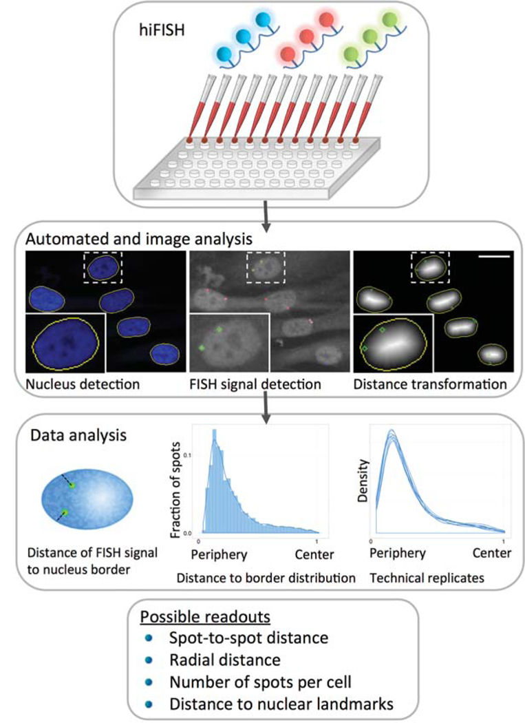
Outline of HIPMap pipeline. Cell plating and FISH (fluorescence in situ hybridization) protocol are performed in a 384-well format in a fully automated manner using fluorescently labeled FISH probes. Representative maximally projected images of z-stacks are analyzed to identify nuclei and detect FISH signals inside each nucleus. The normalized radial distance of each FISH spot from the nucleus border is measured and all distance measurements are combined and plotted as histograms or estimated density curves.
hiFISH
The first step in the HIPMap protocol is hiFISH performed in 96- or 384-well plates using a fully automated liquid handling system. Fibroblasts are plated in 384-well imaging plates at ~80% confluence and are grown for at least 12 h to adhere. For cells in suspension, wells are precoated with poly-L-lysine before plating. Cells are then transfected with siRNAs or expression constructs or treated with compounds depending on the desired experiment. A key feature for successful FISH on a large scale is to streamline the FISH protocol by reducing the number of steps. HiFISHprobes are generated from bacterial artificial chromosomes (BACs) using a standard nick translation protocol with fluorescent nucleotides, thereby eliminating subsequent antibody detection steps as would be needed for biotin-labeled probes or alike. The protocol is also optimized to minimize the number of wash steps to avoid detachment of cells from the plate (Shachar et al. 2015).
Automated Imaging
In the next step, an automated confocal microscope is used to acquire images. In a standard application, samples are imaged in four channels (three probe channels plus DAPI) typically using the 405-, 488-, 561-, and 640-nm laserlineswitha40× waterobjectiveand2× pixel binning. Typically, 60 fields are randomly sampled in a well and six z planes (1-μm intervals) are acquired yielding 1000 to 3000 cells per well, depending on cell size and plating density. The average exposure and imaging time per well using these conditions is ~20 min and the pixel size is 320 nm. Exposure time varies according to cell type and density.
Image Analysis
Images are analyzed in a fully automated fashion to detect cell nuclei and FISH signals. The nucleus border is segmented based on the DAPI staining with high accuracy. FISH spots in all three channels are identified based on detection of local signal maxima in each probe channel. Radial distances from the nuclear edge are measured for every individual FISH signal in a nucleus. Each nucleus undergoes a radial distance transformation in which the border of the nucleus is set as 0 and the center of the nucleus is set as 1. FISH signals are superimposed onto the distance transformation image and their radial coordinates within each nucleus measured (Fig. 1). HIPMap can also measure spot-to-spot Euclidian distances by using the image x andy coordinates of each FISH spot. Spot-to-spot distances can be used to measure distances between alleles or genes or to nuclear landmarks. A detailed description of all image analysis steps is described in Roukos et al. (2013), Burman et al. (2015a), and Shachar et al. (2015).
Data Analysis
To determine the spatial position of a gene inside the nucleus, its distance from the border of the nucleus is measured in hundreds of cells in a population. Individual allele position measurements are combined and plotted as a radial position distribution (Fig. 1). This distribution provides a representation of the overall position of a gene.
For comparison of two distributions, data sets are transformed into cumulative distribution functions (Meaburn and Misteli 2008; Meaburn et al. 2009) and the Kolmo gorov-Smirnov (KS) test (Perlman et al. 2004; Mitchi- son 2005; Smellie et al. 2006) is applied to determine whether the two distributions are different. The KS test is used because it is a nonparametric statistical test that is sensitive to local changes in the shape of the distributions rather than just variations in the mean or median.
To simplify the image analysis, all z-stacks are projected to generate 2D images, and spot coordinates and distances to the nucleus border are measured using only the x andy dimensions. To verify that such an analysis approximates the actual 3D distances and is reliable, we compared spot-to-spot distances in 3D with that in 2D for the same data set. We analyzed human skin fibroblasts and examined the distance between two endogenous loci that reside on two different chromosomes and are not known to interact (LADF and COL1A1; Shachar et al. 2015). Minimal distances between each pair of spots per cell were calculated in projected images or in 3D using six zplanes 1 mm apart (Fig. 2A). The tested cells were treated with a nontargeting siRNA (small interfering RNA) or with an siRNA directed toward LaminA/C and LaminBl that was previously shown to change the radial distribution of LADF and COL1A1 (Shachar et al. 2015). The analysis shows that the distribution of distances between LADF and COL1A1 is similar when analyzed in 2D versus 3D (Fig. 2A). Moreover, when the distance between each pair of spots in 2D was compared with the distance between the same pair in 3D the correlation was very high (Spearman’s p = 0.998) over 7000 measured distances (Fig. 2B). We conclude that spot-to-spot distance 2D analysis of projections is equivalent to 3D analysis.
Figure 2.
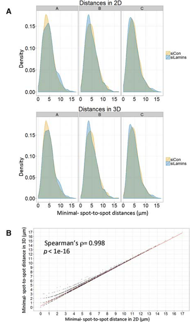
Distance measurement in 2D versus 3D. (A) Comparison of 2D with 3D analysis. Spot-to-spot distance distributions are similar between 2D and 3D analyses. Density curves of spotto-spot distances of LADF and COL1A1 in cells treated with nontargeting siRNA or knocked-down for LaminA/C and LaminB1 are measured in 2D in maximally projected images or using 3D coordinates. Three replicates are shown; each density curve represents at least 1000 distances. (B) Spearman’s correlation between the same minimal spot-to-spot distance measured in 2D versus 3D.
Versatility
To date, HIPMap has been successfully applied to a variety of loci and cell types such as IMR90, MRC5, PC3, and HeLa, as well as lymphocytic cell lines such as ALCL (anaplastic large cell lymphoma) and Jurkat, and to hESCs (human embryonic stem cells). Adherent cells produce better results as a larger number of wash steps during the hiFISH protocol can be applied with minimal loss of cells. The endogenous loci that have been detected by HIPMap include active genes as well as highly repetitive gene deserts (see Fig. 5; Shachar et al. 2015). FISH probe design is limited only by the sequence covered by the specific BAC.
Figure 5.
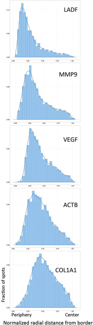
Distributions of endogenous loci. Radial distance distributions (bars) and estimated density curves (lines) of the indicated gene locus. Distributions are generated from more than 600 FISH spots per locus.
QUALITY CONTROL PARAMETERS FOR HIPMap
HIPMap is a robust and highly reproducible method as judged by several quality-control parameters.
False FISH Signal Detection Rate
Because all image analysis steps are fully automated, accurate detection of FISH signals is imperative. To determine the false detection rates of FISH signals, 15 image fields from five hiFISH experiments each containing approximately 300 cells were randomly chosen and the FISH spots identified either visually or by automated image analysis. Comparison of the data sets showed that the false-negative and -positive rates ranged between 0% and 9% for the three channels (Fig. 3A). False signal detection was due to real FISH signals not being detected by the software and fluorescent noise that is identified as signals. Additionally, when the number of FISH spots per cell was analyzed, at least 70% of cells contained two FISH spots as expected for the diploid CRL-1474 human skin fibroblasts used in the analysis (Fig. 3B).
Figure 3.
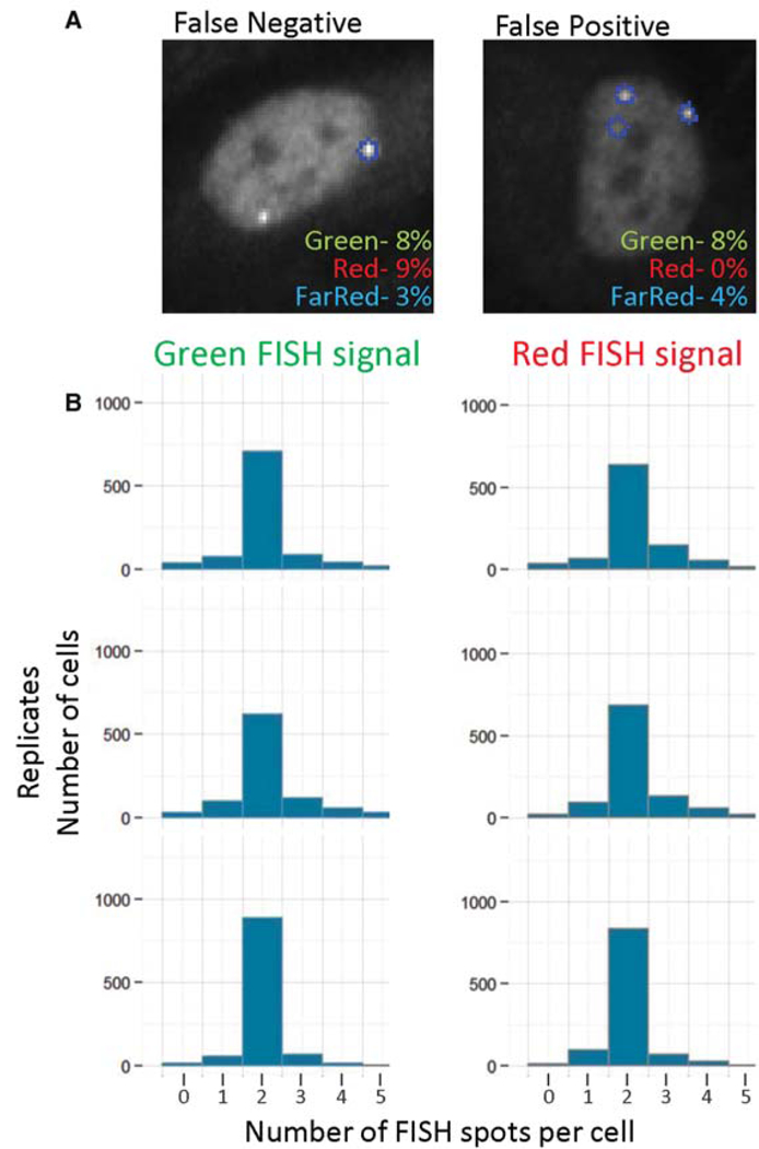
Accuracy of HIPMap image analysis. (A) Representative images of maximally projected z-stacks. The false FISH spot detection ratewas determined by cross comparison of automatically determined spots to manual detection for more than 300 cells in 15 randomly sampled fields. (B) Number of FISH spots detected by image analysis software per cell, calculated for at least 700 cells perwell. Replicate wells are shown for green (488-nm) and red (561-nm) channels
Determination of Minimal Sample Size
HIPMap relies on the statistical analysis of a large number of data points per sample. Although HTI is capable of acquiring a very large number of cells, imaging time becomes a rate-limiting step in large-scale applications. The minimal number of FISH spots required to ensure high statistical fidelity was determined to be approximately 600 FISH spots using a computational simulation (Shachar et al. 2015). Briefly, 9000 FISH spots from nine different wells were pooled and two groups of equal numbers of spots were randomly chosen from this pool. Each two groups of spots were compared to one another using the KS test, and the simulation was repeated 10,000 times for varying spot numbers ranging from 100 to 2000 spots. Using a similar simulation, it is evident that distance distributions of 400 FISH spots or less do not faithfully capture the actual distribution of the population (Fig. 4A; P > 0.05). Distributions generated from less than 400 FISH spots are generally noisy and could be misleading when compared with other distributions generated from low cell numbers.
Figure 4.
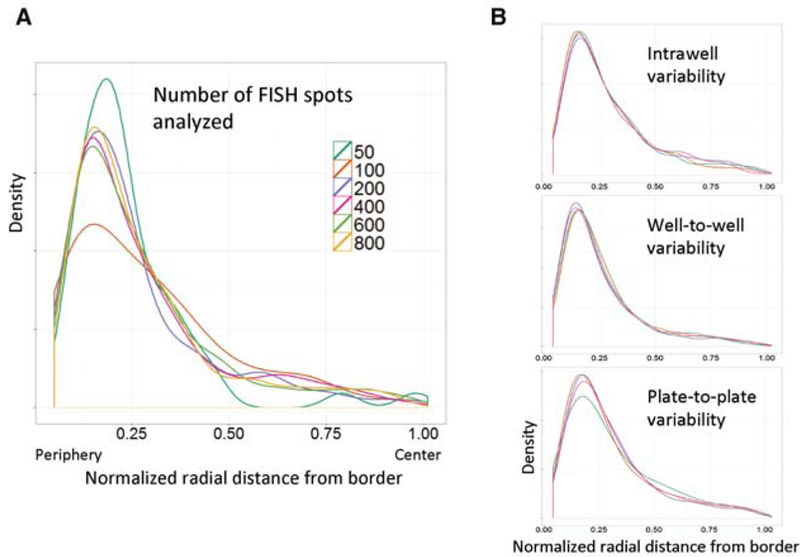
Robustness and reproducibility of HIPMap. (A) Subsampling of data sets demonstrates that radial distance distributions generated from less than 400 FISH spots do not faithfully represent real distribution. Density curves are generated from the indicated number of FISH spots randomly extracted from a pool of 9000 spots from nine replicate wells. (B) Estimated density curves of radial distances generated from more than 600 FISH spots per replicate from the same well, replicate wells on the same plate, or wells in different plates.
Robustness of HIPMap Measurements
Robustness of a method is defined as the degree of similarity among results generated from distinct subpopulations of a data set. HIPMap is highly robust as indicated by the fact that distributions generated from distinct groups of FISH signals randomly sampled from the same well were statistically indistinguishable (P > 0.1) (Fig. 4B). In addition, well-to-well and plate-to-plate variability is minimal (P > 0.1) (Fig. 4B).
MAPPING OF SPATIAL GENE POSITIONS BY HIPMap
Determination of Gene Positions
Representative data sets of HIPMap analysis of five diverse loci in hTERT (human telomerase reverse tran scriptase)-immortalized CRL-1474 human skin fibroblasts are shown in Figure 5. The five loci differ in their chromatin environment, expression levels, and chromosomal location. LADF is a heterochromatic, nonexpressed gene desert located on chromosome 5 previously shown to associate with the nuclear lamina; ACTB and COL1A1 represent active, euchromatic genes and reside on chromosomes 7 and 17, respectively. MMP9 and VEGF are both expressed at low levels in these cells and reside on chromosomes 20 and 6, respectively (Fig. 5). Mapping by HIPMap of these loci identified their distinct radial positions. As expected, most LADF signals are very close to the nuclear periphery with a median radial position of 0.2 (Fig. 5). COL1A1, on the other hand, has a much more internal distribution with a median radial position of 0.53.
Detection of Changes in Gene Positions
A major question in the field concerns the mechanisms that determine the spatial location of gene loci in 3D space. Disruption of candidate mechanisms using RNAi is a possible approach to identify positioning mechanisms. To test whether HIPMap is sensitive enough to detect a change in the position of a gene, the effect of siRNA against LaminA/C and LaminB1, the major components of the nuclear lamina, on the location of the peripheral LADF locus was tested. Simultaneous knock-down of these genes by >90% of their mRNA levels caused a detectable shift in the distribution of LADF (Fig. 6). The median distance from the periphery for the LADF locus changed from 0.2 in cells treated with a non-targeting siRNA to 0.29 in knockdown cells (P < 1 × 10⁻¹⁶). Similar effects of lamin loss were found for three other genes in these cells (Shachar et al. 2015).
Figure 6.
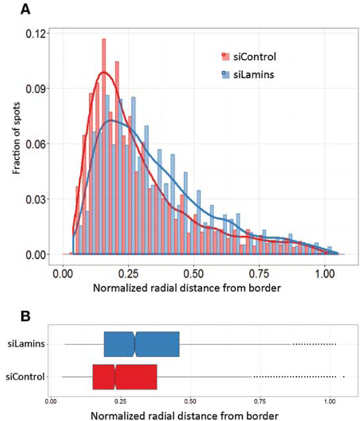
HIPMap detects changes in positioning. (A) Radial distance distributions following siRNA transfection for the indicated gene of the LADF locus. (B) Boxplot of radial distances of the LADF locus to the nucleus border in cells treated with the indicated siRNA for 72 h. Boxes are 25th, 50th (median), and 75 th percentile of the distributions and whiskers extend up to 1.5 interquantile range; outliers are shown as dots.
APPLICATIONS OF HIPMap
HIPMap is a versatile assay that can be used to answer several basic biological questions relevant to chromatin organization as well as more translational questions.
Scaling-Up of HIPMap
A major potential application is the combination of HIPMap with in silico design and synthetic synthesis of FISH oligo probes enabling the scaling-up of gene mapping and screens to probe the location of large sets of genomic targets in a single experiment (Beliveau et al. 2012; Joyce et al. 2012). Large-scale probe design methods, such as Oligopaints, are now available and can be combined with HIPMap. In Oligopaints and its variants (Beliveau et al. 2012,2014,2015), large libraries of DNA oligos tiling genomic regions of interest are designed in silico and chemically synthetized. These libraries of DNA oligos can be either directly labeled with fluoro-phores or designed to include de novo DNA barcodes that can be used as hybridization platforms for fluorescent signal amplification or for multiplexing the number of nucleic acid targets detected in a single sample with imaging approaches (Beliveau et al. 2015; Chen et al. 2015). An obvious obstacle to large-scale FISH experiments is the resulting long imaging times. For example, screening of an siRNA library of 700 candidate genes testing three target loci required a total of 650 imaging hours (Shachar et al. 2015). New generations of high-throughput microscopes with larger camera chips enabling the acquisition of a larger number of cells per field of view and more powerful light sources allowing shorter exposure times will likely overcome this issue in the near future.
RNAi and Small Molecule Screens
We have recently used HIPMap to carry out an siRNA screen to discover factors that contribute to determining the position of four functionally diverse genes in human skin fibroblasts (Fig. 7; Shachar et al. 2015). Using an siRNA library targeting approximately 700 genes encoding nuclear proteins, 2036 wells were imaged and more than three million data points analyzed. The screen identified 50 positioning factors representing a first compendium of cellular proteins that determine the spatial location of human genes (Shachar et al. 2015).
Figure 7.
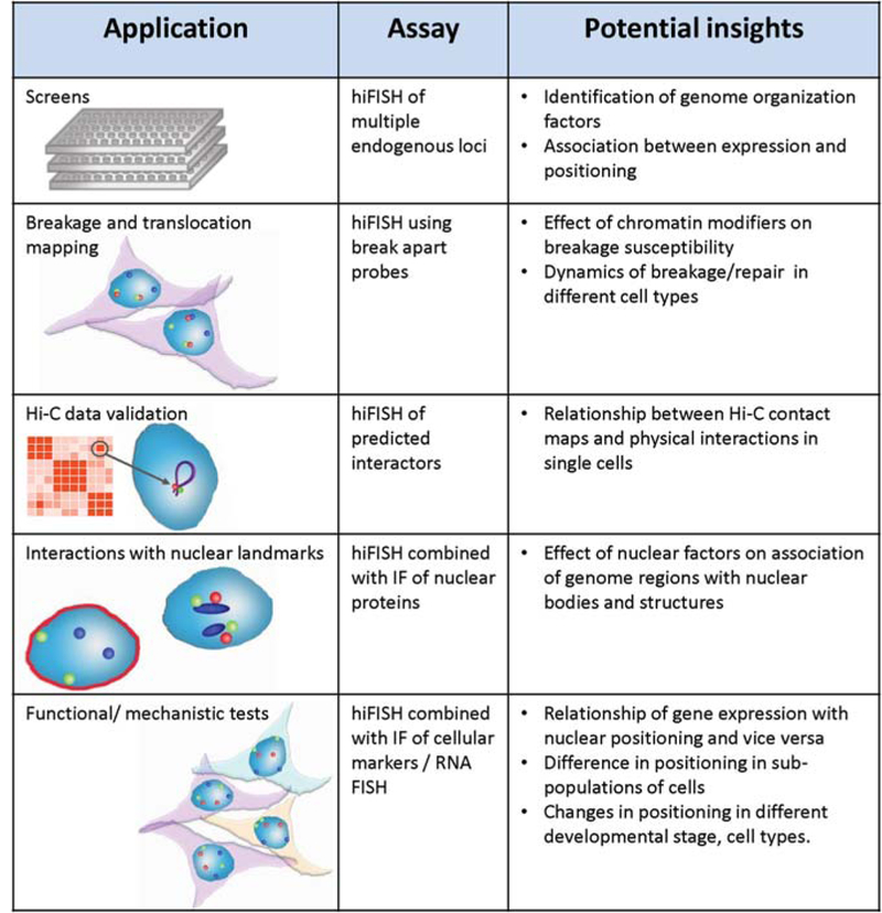
Applications of HIPMap.
Similar screens can be envisioned in any desired adherent cell type and using diverse set of libraries. For example, it would be interesting to explore the effect of interference with cellular signaling pathways on gene positioning. HIP- Map is potentially equally suited for screening of small molecule libraries. Finally, it is foreseeable to apply HIP-Map in combination with CRISPR-based approaches to either knockout or overexpress genes on a large scale.
Systematic Mapping of 3D Distances
HIPMap is ideally suited to measure distances between gene loci. The ability to generate large probe sets targeting custom-defined regions of the genome opens the door to the systematic mapping of locus-to-locus 3D distances between thousands of genomic loci in different biological conditions or in different genetic backgrounds (Fig. 7). The capacity to systematically triangulate the distances of large sets of genome loci has the potential to generate low-resolution 3D genome maps.
Validation of Chromosome Conformation Capture Data Sets
HIPMap is envisioned to become a valuable orthogonal tool to validate chromosome conformation capture (3C) interaction data (Williamson et al. 2014). In one possible scenario, HIPMap could be used to measure 3D distance distributions between a constant genomic locus and a set of tiled FISH probes designed to hybridize at loci positioned at increasing distances away from the bait locus. In addition, Hi-C interactors of similar signal strength, but varying genomic distances, should be systematically analyzed to determine how signal strength and interaction frequencies are related. Alternatively, a large number of loops predicted by high-resolution HiC mapping could be analyzed to determine the percentage of cells that show contacts between genomic regions at the base of the loop. Similarly, interchromosomal interactions can be systematically tested for their prevalence in the cell population.
Determination of Chromosome Breaks and Translocations
Given its capability to measure relational spatial distances of up to three independently labeled genomicloci, HIPMap provides an opportunity to systematically detect rare chromosomal breakage and translocation frequencies in a cell population. An example of such an application has recently been described (Burman et al. 2015a,b) and has led to the finding of an association of increased breakage and translocation frequencies with the presence of specific histone modifications (Burman et al. 2015b). This application of HIPMap could be used to screen for cellular factors involved in the formation of translocations by reverse genetic screens or by using one constant gene as “bait” and by probing hundreds of different “prey” regions representing putative translocation partners (Fig. 7).
HIPMap Combined with Immunofluorescence
HIPMap can also be combined with indirect immunofluorescence (IF) allowing proximity measurements of genomic loci to nuclear bodies and other nuclear landmarks such as the lamina. This allows testing of whether particular nuclear bodies promote the clustering of gene loci and how gene activity is linked to association/dissociation of loci from nuclear bodies. In addition, and more importantly, implementation of combined HIPMap with IF will allow the detection of rare changes in gene repositioning and interactions in sub-populations of cells of interest defined by specific protein biomarkers.
HIPMap-RNA FISH
Finally, coupling HIPMap with RNA FISH provides a single-allele, high-throughput view of the relationships between genome positioning and transcriptional activity. This approach will be particularly important to test on a large scale whether known changes in gene expression associated with physiological changes are accompanied by changes in radial position of the corresponding genomic locus (Therizols et al. 2014).
CONCLUSION
The HIPMap pipeline is an optimized tool to map the spatial positions of genes in the intact cell nucleus. The availability of a method that combines the power of direct visualization of gene loci and single-cell imaging with the ability to interrogate genomes at a large-scale overcomes some of the limitations inherent to the two major methods, microscopy and 3C technology, that have been used to probe higher-order genome organization. HIPMap is a highly modular technology, and combination of HIPMap with the development of more complex probe libraries, with other detection methods, and with the use of genetic tools will furtherenhance the impact ofthe method. Regardless of the nature of future applications, HIPMap has the potential to contribute significantly to the elucidation of genome structure and function.
ACKNOWLEDGMENTS
We thank Karen Meaburn for help with developing hiFISH and members of the Misteli laboratory for helpful discussions and comments. This research was supported by the Intramural Research Program of the National Institutes of Health (NIH), the National Cancer Institute (NCI), and the Center for Cancer Research.
REFERENCES
- Beliveau BJ, Joyce EF, Apostolopoulos N, Yilmaz F, Fonseka CY, McCole RB, Chang Y, Li JB, Senaratne TN, Williams BR, et al. 2012. Versatile design and synthesis platform for visualizing genomes with Oligopaint FISH probes. Proc Natl AcadSci 109: 21301–21306. [DOI] [PMC free article] [PubMed] [Google Scholar]
- Beliveau BJ, Apostolopoulos N, Wu CT. 2014. Visualizing genomes with Oligopaint FISH probes. Curr Protoc Mol Biol 105: Unit 14 23. [DOI] [PMC free article] [PubMed] [Google Scholar]
- Beliveau BJ, Boettiger AN, Avendaiio MS, Jungmann R, McCole RB, Joyce EF, Kim-Kiselak C, Bantignies F, Fonseka CY, Erceg J, et al. 2015. Single-molecule super-resolution imaging of chromosomes and in situ haplotype visualization using Oligopaint FISH probes. Nat Commun 6: 7147. [DOI] [PMC free article] [PubMed] [Google Scholar]
- Burman B, Misteli T, Pegoraro G. 2015a. Quantitative detection of rare interphase chromosome breaks and translocations by high-throughput imaging. Genome Biol 16: 146. [DOI] [PMC free article] [PubMed] [Google Scholar]
- Burman B, Zhang ZZ, Pegoraro G, Lieb JD, Misteli T. 2015b. Histone modifications predispose genome regions to breakage and translocation. Genes Dev 29: 1393–1402. [DOI] [PMC free article] [PubMed] [Google Scholar]
- Cavalli G, Misteli T. 2013. Functional implications of genome topology. Nat Struct Mol Biol 20: 290–299. [DOI] [PMC free article] [PubMed] [Google Scholar]
- Chen KH, Boettiger AN, Moffitt JR, Wang S, Zhuang X. 2015. RNA imaging. Spatially resolved, highly multiplexed RNA profiling in single cells. Science 348: aaa6090.. [DOI] [PMC free article] [PubMed] [Google Scholar]
- Conrad C, Gerlich DW. 2010. Automated microscopy for high content RNAi screening. J Cell Biol 188: 453–461. [DOI] [PMC free article] [PubMed] [Google Scholar]
- Cremer T, Cremer M. 2010. Chromosome territories. Cold Spring Harb Perspect Biol 2: a003889. [DOI] [PMC free article] [PubMed] [Google Scholar]
- Dekker J, Misteli T. 2015. Long-range chromatin interactions In Epigenetics, 2nd ed. (ed. Allis CD, et al. ), pp. 507–528. Cold Spring Harbor Laboratory Press, Cold Spring Harbor, NY. [DOI] [PMC free article] [PubMed] [Google Scholar]
- Dekker J, Marti-Renom MA, Mirny LA. 2013. Exploring the three-dimensional organization of genomes: Interpreting chromatin interaction data. Nat Rev Genet 14: 390–403. [DOI] [PMC free article] [PubMed] [Google Scholar]
- de Wit E, de Laat W. 2012. A decade of 3C technologies: Insights into nuclear organization. Genes Dev 26: 11–24. [DOI] [PMC free article] [PubMed] [Google Scholar]
- Dixon JR, Selvaraj S, Yue F, Kim A, Li Y, Shen Y, Hu M, Liu JS, Ren B. 2012. Topological domains in mammalian genomes identified by analysis of chromatin interactions. Nature 485: 376–380. [DOI] [PMC free article] [PubMed] [Google Scholar]
- Joyce EF, Williams BR, Xie T, Wu CT. 2012. Identification of genes that promote or antagonize somatic homolog pairing using a high-throughput FISH-based screen. PLoS Genet 8: e1002667. [DOI] [PMC free article] [PubMed] [Google Scholar]
- Meaburn KJ, Misteli T. 2008. Locus-specific and activity-independent gene repositioning during early tumorigenesis. J Cell Biol 180: 39–50. [DOI] [PMC free article] [PubMed] [Google Scholar]
- Meaburn KJ, Gudla PR, Khan S, Lockett SJ, Misteli T. 2009. Disease-specific gene repositioning in breast cancer. J Cell Biol 187: 801–812. [DOI] [PMC free article] [PubMed] [Google Scholar]
- Misteli T 2007. Beyond the sequence: Cellular organization of genome function. Cell 128: 787–800. [DOI] [PubMed] [Google Scholar]
- Misteli T 2013. The cell biology of genomes: Bringing the double helix to life. Cell 152: 1209–1212. [DOI] [PMC free article] [PubMed] [Google Scholar]
- Mitchison TJ. 2005. Small-molecule screening and profiling by using automated microscopy. Chembiochem 6: 33–39. [DOI] [PubMed] [Google Scholar]
- Nagano T, Lubling Y, Stevens TJ, Schoenfelder S, Yaffe E, Dean W, Laue ED, Tanay A, Fraser P. 2013. Single-cell HiC reveals cell-to-cell variability in chromosome structure. Nature 502: 59–64. [DOI] [PMC free article] [PubMed] [Google Scholar]
- Perlman ZE, Slack MD, Feng Y, Mitchison TJ, Wu LF, Altschuler SJ. 2004. Multidimensional drug profiling by automated microscopy. Science 306: 1194–1198. [DOI] [PubMed] [Google Scholar]
- Roukos V, Misteli T, Schmidt CK. 2010. Descriptive no more: The dawn of high-throughput microscopy. Trends Cell Biol 20: 503–506. [DOI] [PMC free article] [PubMed] [Google Scholar]
- Roukos V, Voss TC, Schmidt CK, Lee S, Wangsa D, Misteli T. 2013. Spatial dynamics of chromosome translocations in living cells. Science 341: 660–664. [DOI] [PMC free article] [PubMed] [Google Scholar]
- Sexton T, Yaffe E, Kenigsberg E, Bantignies F, Leblanc B, Hoichman M, Parrinello H, Tanay A, Cavalli G. 2012. Three-dimensional folding and functional organization principles of the Drosophila genome. Cell 148: 458–472. [DOI] [PubMed] [Google Scholar]
- Shachar S, Voss TC, Pegoraro G, Sciascia N, Misteli T. 2015. Identification of gene positioning factors using high-throughput maging mapping. Cell 162: 911–923. [DOI] [PMC free article] [PubMed] [Google Scholar]
- Smellie A, Wilson CJ, Ng SC. 2006. Visualization and interpretation of high content screening data. J Chem Inf Model 46: 201–207. [DOI] [PubMed] [Google Scholar]
- Therizols P, Illingworth RS, Courilleau C, Boyle S, Wood AJ, Bickmore WA. 2014. Chromatin decondensation is sufficient to alter nuclear organization in embryonic stem cells. Science 346: 1238–1242. [DOI] [PMC free article] [PubMed] [Google Scholar]
- Williamson I, Berlivet S, Eskeland R, Boyle S, Illingworth RS, Paquette D, Dostie J, Bickmore WA. 2014. Spatial genome organization: Contrasting views from chromosome conformation capture and fluorescence in situ hybridization. Genes Dev 28: 2778–2791. [DOI] [PMC free article] [PubMed] [Google Scholar]