

Abstract
In single-molecule Förster resonance energy transfer (FRET) spectroscopy, the dynamics of molecular processes are usually determined by analyzing the fluorescence intensity of donor and acceptor dyes. Since FRET efficiency is related to fluorescence lifetimes, additional information can be extracted by analyzing fluorescence intensity and lifetime together. For fast processes where individual states are not well separated in a trajectory, it is not easy to obtain the lifetime information. Here, we present analysis methods to utilize fluorescence lifetime information from single-molecule FRET experiments, and apply these methods to three fast-folding, two-state proteins. By constructing 2D FRET efficiency-lifetime histograms, the correlation can be visualized between the FRET efficiency and fluorescence lifetimes in the presence of the sub-microsecond to millisecond dynamics. We extend the previously developed method for analyzing delay times of donor photons to include acceptor delay times. In order to determine the kinetics and lifetime parameters accurately, we used a maximum likelihood method. We found that acceptor blinking can lead to inaccurate parameters in the donor delay time analysis. This problem can be solved by incorporating acceptor blinking into a model. While the analysis of acceptor delay times is not affected by acceptor blinking, it is more sensitive to the shape of the delay time distribution resulting from a broad conformational distribution in the unfolded state.
Graphical Abstract
Introduction
Single-molecule fluorescence spectroscopy is a powerful tool to detect individual molecular events. It has been widely used to monitor complex molecular interactions1–4 and to measure conformational dynamics of macromolecules such as proteins5–13 and nucleic acids.14–20 When more than one fluorophore are attached to a molecule, conformational states can be characterized by the Förster resonance energy transfer (FRET) efficiency determined by the distance between two fluorophores.21,22 The FRET efficiency is usually calculated from the relative fluorescence intensity of two dyes. In an experiment with pulsed laser excitation, fluorescence lifetime can also be measured, from which one can extract additional information. Seidel and coworkers have pioneered the use of two-dimensional (2D) lifetime-FRET efficiency histograms to describe the correlation between the donor fluorescence lifetime and the FRET efficiency in a bin.9,23 Schuler and coworkers used 2D lifetime-FRET efficiency histograms to select fluorescence bursts from unfolded protein molecules for the analysis of donor and acceptor lifetimes to obtain distance distributions between donor and acceptor.24,25 Ha and coworkers have identified various conformational states and intermediates during the transcription initiation process from the analysis of fluorescence lifetime trajectories.26 1D and 2D fluorescence lifetime correlation analyses have also been used to distinguish different species in a mixture27,28 or to probe fast molecular processes on the microsecond to millisecond time scale.29,30 Recently, a rigorous theory has been developed for analyzing FRET efficiency and donor fluorescence lifetime histograms.31
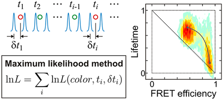
In this paper, we describe an analysis of single-molecule photon trajectories using both histogram and photon-by-photon analyses. An experimentally obtained photon trajectory consists of photons with registered color (donor or acceptor), absolute time of arrival at the detector (arrival time), and difference between the time of the laser excitation pulse and arrival time (delay time). In a histogram analysis, a photon trajectory is divided into bins of equal bin time, and the FRET efficiency (the fraction of the acceptor photons) and the mean donor and acceptor delay times (fluorescence lifetimes) are calculated for each bin. The shape of the histogram depends on the bin time. In the absence of any dynamics, the distribution is centered on the diagonal of the 2D plot. Fluctuations of the inter-dye distance induce a deviation from the diagonal line. From the analysis of this deviation, it is possible to obtain insight into molecule’s dynamics and photophysics.9,23 For example, a positive shift of the distribution above the diagonal is an indication of a broad distribution of donor-acceptor distances that inter-convert on the sub-microsecond time scale.25,32 When there are slow transitions between, say, folded and unfolded states of a protein, the 2D histogram has two peaks corresponding to the states. When transitions occur on the same time scale as the bin time, the distribution is located near a two-state dynamic line,9,31,33 which is curved (concave downwards). We extend the analysis of the 2D histograms to include the delay times of the acceptor photons.
For the sufficiently slow dynamics, the 2D histograms yield an accurate measure of the FRET efficiencies, lifetimes, and relative populations of the states. When the interconversions between states are fast and the states cannot be resolved, a photon-by-photon analysis using the maximum likelihood method can be used to get the parameters of a model that describes molecule’s dynamics.34 This method does not involve binning of trajectories. It has been successfully applied to analyze fast conformational dynamics of proteins33,35–38 and DNA.19,39 Here we extend this method to include information from the donor and acceptor delay times. By analyzing colors, arrival times, and delay times of individual photons, the maximum likelihood method determines the FRET efficiency, the mean delay times of the states, and the rate coefficients for the transitions between them. In the maximum likelihood analysis, it is important to choose a proper model to describe distance fluctuations and photophysics. In our previous analyses without delay times35 we used the fact that the processes fast compared to the inter-photon times are averaged out and affect only the apparent FRET efficiencies.34 This simplifies the model since only the states are explicitly included that interconvert on time scale slower than the photon detection rate, which is less than one photon/microsecond at the illumination intensities generally employed. For example, fast acceptor blinking does not affect the extracted folding and unfolding rate coefficients unless the rate becomes comparable to the inter-photon times and the population in the dark state exceeds 10%.33 In contrast, the maximum likelihood analyses with delay times is more challenging because conformational dynamics on the submicrosecond time scale and fast photophysics influence the distributions of the delay times that enter the likelihood function. With the aim of getting the simplest models that would provide a description consistent with the experimental data, we used three kinetics models: a two-state, four-state, and modified two-state model. The two-state model consists of the folded and unfolded states. In the four-state model, each of the two states consists of the bright and dark states of the acceptor fluorophore. The modified two-state model consists of the folded and unfolded states but the FRET efficiencies and lifetimes are modified to incorporate the acceptor blinking effect. We also employed two different approaches to the analysis. In the first, all parameters were determined simultaneously. In the second, we determined the FRET efficiency and folding kinetics parameters first using photon color information only, and with these parameters being fixed, subsequently determined fluorescence lifetimes. This latter method is faster and simpler.
We applied these methods to the analysis of three two-state proteins with different folding rates (α3D, gpW, and WW domain, Figure 1). The most accurate parameters were determined from the analysis using the four-state kinetics model that includes acceptor blinking explicitly, which was necessary for analyzing fast folding proteins such as the WW domain. For the system with moderately fast kinetics compared to the photon count rate, such as α3D and gpW, accurate lifetime parameters could also be determined using a simpler, modified two-state analysis. From the simulation of photon trajectories with various rates and acceptor dark state populations, we determined when and how the extracted parameters deviate from the true values. We also investigated in simulations how the assumptions on the shape of the delay time distribution affect the extracted parameters.
Figure 1.

Immobilization of proteins and amino acid sequences. (a) Dye-labeled protein molecules are immobilized on a polyethylene glycol (PEG)-coated glass surface via a biotinstreptavidin-biotin linkage. (b) Dyes are attached to the cysteine residues (red) and a biotin molecule to the lysine residue (blue) in the 15-residue biotin accepting sequence (AviTag). α3D and gpW were labeled with Alexa 488 and Alexa 594 and the WW domain was labeled with Alexa 488 and Atto 647N.
Materials, methods, and theory
Materials.
The expression, purification, and dye-labeling of α3D and the WW domain were described previously.35,36 α3D was labeled with Alexa Fluor 488/Alexa Flour 594 pair and the WW domain with Alexa Fluor 488/Atto 647N pair. (Figure 1)
A synthetic gene encoding 62 amino acids of lambda prophage-derived head-to-tail joining protein W (gpW)40–42 flanked by cysteine residues at its termini and an N-terminal biotin acceptor peptide (Avidity LLC, Aurora, CO) followed by a spacer sequence (Figure 1) was cloned between the Nde1 and BamH1 sites of pET11a vector (Novagen, San Diego, CA). The resulting construct (Avi-gpW) was verified by DNA sequencing.
The expression construct Avi-gpW and a plasmid with an isopropylthiogalactoside (IPTG) inducible birA gene to over-express the biotin ligase (Avidity LLC) were co-transformed into E.coli BL-21 (DE3; Stratagene, La Jolla, CA). Cells were grown in Luria-Bertani medium, and expression was induced at an absorbance of 0.7 monitored at 600 nm with a final concentration of 1 mM IPTG for a period of 3–4 h. A final concentration of 50 μM d-biotin (Sigma, St. Louis, MO) was added to the medium ~ 30 min before induction. Typically, cells harvested from a 500-mL culture were lysed by uniform suspension in 20 mL of bacterial protein extraction reagent (B-PER, Pierce, Rockford, IL) and sonication. The lysate was centrifuged at 20,000g for 30 min at 4°C. The supernatant was subjected to affinity chromatography using streptavidin Mutein matrix (Roche Diagnostics GmbH, Mannheim, Germany). The column was equilibrated and washed extensively, after passing the lysate, with 1X PBS (1.7 mM KH2PO4, 5 mM Na2HPO4, 150 mM NaCl, pH 7.4) and the biotinylated Avi-gpW was eluted in 1X PBS containing 2 mM d-biotin. The eluted protein was adjusted to a final concentration of 1 mM DTT, concentrated using centriprep-YM10 devices (Millipore Corp, Bedford, MA) to ~ 1.5 mL and loaded onto a Superdex-75 column (1.6 cm × 60 cm; GE HealthCare, Piscataway, NJ) equilibrated in 25 mM Tris-HCl, pH 7.5 and 1 mM DTT at a flow-rate of 1.5 mL/min at room temperature. Peak fractions were analyzed by SDS-PAGE, combined and subjected to reverse-phase HPLC on POROS 20 R2 resin (Life Technologies, Grand Island, NY) and eluted using a linear gradient from 99.95% water (v/v) and 0.05% TFA to 60% acetonitrile (v/v), 0.05% TFA (v/v) and 39.95% water (v/v) over a period of 16 min at a flow rate of 4 mL/min. Aliquots of the peak fraction were lyophilized and stored at −70°C. Typically, labeling with Alexa Fluor 488 and Alexa Fluor 594 was carried out with at least 5-fold molar excess of dye in 6M guanidine hydrochloride (GdmCl), 50 mM Tris-HCl, pH 8 for ~2.5 hours. The reaction was terminated by the addition of 2-mercapto-ethanol (Sigma) to a final concentration of 10 mM, incubated for 10 min, followed by fractionation on a Superdex-30 column (1cm × 30 cm, , GE HealthCare) in 0.5X PBS to remove the unreacted dye. Peak fractions corresponding to the labeled protein were subjected to anion-exchange chromatography (Mono Q 5/50 GL, GE HealthCare) and monitored with 3 wavelengths to separate and identify Avi-gpW bearing the donor-acceptor pair from the donor or acceptor only fractions.
Single-molecule spectroscopy.
Single-molecule FRET experiments were performed using a confocal microscope system (MicroTime200, Picoquant) with an oil-immersion objective (PlanApo, NA 1.4, × 100, Olympus). Donor dyes were excited by a 485 nm diode laser (LDH-DC-485, PicoQuant) in the pulsed mode at 20 MHz. Molecules were illuminated at ~2 kW/cm2. Donor and acceptor fluorescence was split into two channels and focused through optical filters (ET525/50m for the donor and E600LP for the acceptor, Chroma Technology) onto photon-counting avalanche photodiodes (SPCM-AQR-15, PerkinElmer Optoelectronics).
Biotinylated protein molecules were immobilized on a biotin-embedded, polyethyleneglycol-coated glass coverslip (Bio_01, Microsurfaces Inc.) via a biotin (surface)-streptavidin-biotin (protein) linkage. The experiments were performed near the midpoints of GdmCl denaturation, 2.3 M, 2.5 M, and 2 M in 50 mM HEPES buffer (pH 7.6) for α3D, gpW, and the WW domain, respectively. To reduce dye photobleaching and blinking, 1 mM of L-ascorbic acid and methyl viologen43 (α3D and WW domain) or 10 mM cysteamine and 100 mM β-mercaptoethanol44 (gpW) were added.
Additional details for the optical setup and single-molecule experiments have been described elsewhere.45,46
Two-dimensional FRET efficiency and fluorescence lifetime histograms.
Consider a molecule labeled with a donor and an acceptor fluorophore. Excitation of the donor by a pulsed laser results in the emission of either a donor or an acceptor photon, depending on the distance between the fluorophores. A photon trajectory is a sequence of photons with recorded colors (i.e., donor or acceptor), arrival times, and delay times (see Figure 2(a)). To construct a histogram, the photon trajectory is divided into bins of equal duration (the bin time). The FRET efficiency in a bin is defined as E = NA/(NA + ND), where NA and ND are the numbers of acceptor and donor photons in a bin. The mean donor (acceptor) delay time in a bin, τD (τA), is defined as the mean of all donor (acceptor) delay times (δt) in that bin. All of these quantities are random and vary from bin to bin, mainly due to the finite numbers of photons (shot noise) and the fluctuations of the distance between the donor and acceptor labels. Below we neglect shot noise and focus on the limit of a large number of photons in every bin.
Figure 2.

(a) A schematic representation (not to scale) of a sequence of donor (green) and acceptor (red) photons detected after pulsed laser excitations (blue dashed lines). For each photon, the arrival time (t) and the time δt between the laser pulse and the photon (delay time) is recorded. (b) Resonance energy transfer from donor to acceptor. After laser excitation (DA → D*A), the donor decays to the ground state or the energy is transferred to the acceptor (D*A → DA*) and decays to the ground state. kA and kD are the sum of the rates of the non-radiative (black solid arrows) and radiative (rippled arrows) decays of the acceptor and donor, respectively, which are the reciprocal excited-state lifetimes of the acceptor (τA0) and the donor in the absence of the acceptor (τD0). kET is the energy transfer rate from the donor to the acceptor. The mean donor delay time is equal to the donor lifetime, τD. The mean acceptor delay time is τA = τDA + τA0, where τDA is the donor excited-state lifetime on condition that the energy is transferred to the acceptor, which is not the same as the donor lifetime measured from the donor photons τD when there are fluctuations in kET (see eqs 6 and 7). (c) Two-state kinetic model and (d) four-state kinetic model that includes acceptor blinking. Subscripts b and d stand for the bright and dark states of the acceptor, respectively. (e) The instrument response functions (IRF) of the donor (green circle) and acceptor (orange circle) detection channels and the fits to the Gamma distribution (eq 20) (red and blue lines). t0 = 0.225 ns, a = 6.03 and kγ = 8.91 ns−1 for the donor channel and t0 = 0.234 ns, a = 6.84 and kγ = 11.0 ns−1 for the acceptor channel. (See Supporting Information (SI) for the dependence of the IRF on the count rate and wavelength of photons.) (f and g) Donor and acceptor delay time distributions from the photon trajectories of α3D. The experimental data (grey) was fitted to the convolution (red) of IRF (green dashed line) with a biexponential function for the distribution in the donor channel (f). The acceptor delay time distribution was fitted to the convolution of IRF (green) with a function similar to eq 15, which consists of the biexponential donor lifetime distribution and the single-exponential acceptor excited-state lifetime distribution (g).
Both donor and acceptor delay times are related to the lifetime of the donor excited state. After excitation, the donor can either emit a photon or transfer its excitation energy to the acceptor (see Figure 2(b)). The mean donor delay time, τD, is the excited-state lifetime on condition that the excited state decays by emitting a donor photon. The mean acceptor delay time, τA, is the sum of the acceptor excited-state lifetime, τA0, and the lifetime of the donor excited state on condition that it decays over the energy transfer channel, denoted by τDA. In general, these two conditional lifetimes of the donor excited state, τD and τDA = τA - τA0, are different. We refer to them as the fluorescent lifetimes obtained using donor or acceptor delay times.
When the distance, r, between the donor and acceptor is fixed, the distribution of the donor delay times (δt) is single-exponential, PD(δt) ∝ exp(−(kET + kD)δt), where kET = kD(R0/r)6 is the energy transfer rate, R0 is the Förster radius, and kD is the donor decay rate in the absence of the acceptor (see Figure 2(b)). The mean of this distribution is the lifetime of the donor excited state, τD = (kET + kD)−1, which is related to the FRET efficiency E = kET/(kET + kD) by22
| (1) |
where is the donor lifetime in the absence of the acceptor.
The acceptor fluorophore is excited by the energy transfer from the donor, so that the distribution of the acceptor delay times is biexponential, PA(δt) ∝ exp(−kAδt) - exp(−(kET + kD)δt), with the mean delay time equal to where τA0 = kA−1 is the lifetime of the acceptor excited state. Therefore,
| (2) |
Equations (1) and (2) relate the FRET efficiency and the mean delay times (fluorescence lifetimes) when there is no shot noise and no conformational dynamics. They correspond to the diagonals on the 2D histograms of the FRET efficiency E and the relative lifetimes, which are obtained from the donor delay times, τD/τD0, or acceptor delay times, (τA - τA0)/τD0. When there are no dynamics, these lifetimes are the same.
Fluctuations of the inter-dye distance result in deviations of the FRET efficiencies and lifetimes from the diagonal line.9,23,25 To include fluctuations, consider a molecule that can emit photons from several states. Each state s is characterized by the acceptor and donor photon count rates (the mean numbers of photons per unit time when the molecule is in state s), nAs and nDs, and by the mean acceptor and donor delay times, τAs and τDs. A state s can be any molecular state with a different FRET efficiency such as distinct conformational states with different inter-dye distances or photophysical states of fluorophores. The apparent FRET efficiency in state s is defined as Es = nAs/(nAs + nDs).
The FRET efficiencies and donor and acceptor delay times in consecutive bins of a photon trajectory can change due to transitions between states. Let θs be the fraction of time spent in state s during the bin time, Σsθs = 1. This fraction is a random quantity and depends on the time scale of the transitions compared to the bin time. When a state does not change during the bin time, θs is 0 or 1. When transitions are fast and many states are visited during the bin time, θs converges to the equilibrium population in state s. The FRET efficiency and delay times in a bin can be written as
| (3a) |
| (3b) |
| (3c) |
These equations will be used to derive new relationships between FRET efficiencies and delay times.
Consider a molecule with two states, folded and unfolded, so that s = F, U in the above equations. Excluding the fractions θF and θU = 1 - θF from eqs 3a and 3b, and using the apparent FRET efficiencies in the folded and unfolded states, EU = nAU/(nAU + nDU) and EF = nAF/(nAF + nDF), we have
| (4) |
This equation relates the mean donor delay time τD and the FRET efficiency E. This is equivalent to eq 8 in Ref.31 and reduces to eq 9d in Ref.23 in the special case when there are no sub-microsecond dynamics in the states.
Similarly, using eqs 3a and 3c, the relationship between the FRET efficiency and the acceptor delay times is:
| (5) |
Note that eq 5 for the mean acceptor delay times can be obtained from eq 4 for the donor delay times by the simple replacements E → 1 − E, EU → 1 − EU, and EF → 1 − EF.
Equation (4) and (5) define the two-state dynamic lines connecting the folded and unfolded peaks of the 2D histograms. They show the location of the distribution in the absence of shot noise. When the bin time is sufficiently short, the distribution is located near the points corresponding to the folded and unfolded states. When the bin time is comparable to the transition time between the two states, the FRET efficiencies and delay times are distributed along the two-state dynamic line. The lines deviate from the diagonal due to transitions between folded and unfolded states. The donor two-state line is concave downward, whereas the acceptor line is concave upward.
Now we specify the FRET efficiencies and mean delay times in the folded and unfolded states. If we assume that there are no dynamics in the folded state, then τDF/τD0 = (τAF - τA0)/τD0 = 1 - EF, i.e., the folded peak is located on the diagonal of both 2D plots. In the unfolded state, the conformational fluctuation on the submicrosecond time scale leads to a different relationship. This can be found using eq 3b, where s now refers to the substates in the unfolded state that correspond to various donor-acceptor distances. Since the unfolded polypeptide chain dynamics occur on a time scale much shorter than inter-photon times,47 the fraction θs in eq 3 can be replaced with the normalized equilibrium population ps of a distribution of substates s in the unfolded state. Taking into account that nAs = nUEs, nDs = nU(1 - Es), τDs/τD0 = 1 - Es, where Es is the FRET efficiency of substate s and nU = nAs + nDs is the total count rate in the unfolded state (assumed to be independent of s), results in31
| (6) |
Here, EU = ΣsEsps is the mean FRET efficiency in the unfolded state, σU2 = ΣsEs2ps - EU2 is the variance of the FRET efficiency due to the fluctuations of the donor-acceptor distance in the unfolded state.
The mean acceptor delay time and the corresponding fluorescence lifetime in the unfolded state is obtained similarly using eq 3c and τAs = τA0 + τDs:
| (7) |
Here the FRET efficiency variance σU2 is the same as that in eq 6.
Thus fluctuations in the unfolded state lead to an increase in the mean donor delay time, eq 6, and to a decrease in the mean acceptor delay time, eq 7, which results in the shift of the peak corresponding to the unfolded state above (below) the diagonal on the 2D histograms with donor (acceptor) delay times. This happens because an increase in the donor-acceptor distance, which results in a longer excited-state lifetime, also increases the donor photon counts, but decreases the acceptor counts.
While the variables in eqs 4 and 5 can be apparent values without any correction, those in eqs 6 and 7 are “true” lifetimes and FRET efficiencies, and therefore, the extracted parameters should be corrected for the background noise, crosstalk, and γ-factor (the ratio of the quantum yields and detection efficiencies of the acceptor and donor photons) before using these equations.
Maximum likelihood method.
Given a model, a maximum likelihood method can be used to find the model parameters that are most consistent with the observed photon trajectories by maximizing an appropriate likelihood function. The likelihood function for the jth photon trajectory that uses photon colors, arrival, and delay times is31,34
| (8) |
where Nj is the number of photons in the jth trajectory, ci is the color of the ith photon (donor or acceptor), and ti - ti-1 is a time interval between the (i-1)th and ith photons (Figure 2(a)). Here K is the rate matrix, the photon color matrix F depends on the color c of a photon as F(acceptor) = E and F(donor) = I – E, where E is a diagonal matrix with the apparent FRET efficiencies of the individual states on the diagonal, I is the unity matrix, 1T is the unit row vector (T means transpose), and peq is the vector of equilibrium populations. The matrix P(c, δt) is a diagonal matrix with the elements PDs(δt) (c = donor) or PAs(δt) (c = acceptor) depending on the color of a photon. The diagonal elements are the normalized delay time (δt) distributions of the donor and acceptor photons, respectively, when a molecule is in state s.
The likelihood function that uses only photon colors and arrival times is given by eq 8 with the delay time distributions set to unity, P(c, δt) = I. The calculation of the likelihood function is performed using the diagonalization of the matrix exponential in eq 8 as described in Ref.34. Practically, the log-likelihood function is calculated by summing individual log-likelihoods as lnL = Σj lnLj.
For the two-state model describing folding (see Figure 2(c)), the matrix of FRET efficiencies, the rate matrix, and the vector of the equilibrium populations are given by
| (9) |
where pF = kF/(kF + kU) is the equilibrium population of the folded state. They involve four model parameters: the rate coefficients, kF and kU, (or the relaxation rate, k = kF + kU, and the population, pF) and the apparent FRET efficiencies of the folded and unfolded states, EF and EU.
The above rate matrix K is not affected by the processes that are fast compared to the inter-photon times such as dynamics in the unfolded state, as well as background noise. These processes only alter the measured FRET efficiencies from the true values.34
The matrices of the delay time distributions for the two-state model are
| (10) |
The acceptor and donor delay time distributions in the folded and unfolded states, PAF, PAU, PDF, and PDU, are influenced by the instrument response function (IRF) and background noise (see sections below). The shape of the distribution also depends on the fast dynamics. Suppose that the unfolded state consists of many substates s that interconvert on a timescale faster than inter-photon times (submicrosecond) but slower than the excited-state lifetime (nanosecond). Then the donor delay time distribution in the unfolded state is a weighted sum of single-exponential distributions with respect to the substates:
| (11a) |
| (11b) |
where τDs is the lifetime of the donor excited state when the molecule is in substate s of the unfolded state, fDs is the probability that the donor photon was emitted from substate s (the fractional contribution of substate s),22,31† nDs is the donor photon count rate, ps is the equilibrium population in substate s. The acceptor delay time distribution in the unfolded state is a weighted sum of double-exponential distributions with respect to the substates:
| (12a) |
| (12b) |
where τAU0 is the lifetime of the acceptor excited state when the molecule is in the unfolded state, fAs is the probability that the acceptor photon was emitted from substate s, and nAs is the acceptor photon count rate.
The above delay time distributions contain too many unknown parameters, which makes optimization of the likelihood function complicated. To simplify the analysis, we assume that the donor delay time distribution is single-exponential in both folded and unfolded states:
| (13) |
By optimizing the likelihood function with respect to τDF and τDU, we expect to get the mean (i.e., averaged over fast processes) lifetimes of the donor excited state (which decays to the ground state by emitting a donor photon) in the folded and unfolded states, respectively.
The acceptor delay time distribution is assumed to be double exponential:
| (14) |
where τAF(U)0 is the lifetime of the acceptor excited state, which depends on the microscopic environment when the molecule is in the folded (F) or unfolded (U) state.46,48 In this way we expect to get mean lifetimes τDFA and τDUA, which are the lifetimes of the donor excited state on the condition that the state decays to the acceptor excited state.
The simplified single-exponential and double-exponential delay time distributions should be considered as fitting functions used to extract the mean excited-state lifetimes τDF and τDU from the donor delay times and τDFA and τDUA from the acceptor delay times. We checked the validity of our procedure by simulations and by increasing the number of exponents in the delay time distribution. Specifically, assuming a double-exponential distribution of the donor excited-state lifetime, we also consider the following distribution for the acceptor delay times in the unfolded state:
| (15) |
Here all three lifetimes and the fraction α are determined. The average lifetime is then calculated as τDUA = ατDU1A + (1 – α)τDU2A.
The new lifetime parameters in the delay time distributions are related to the FRET efficiencies of the states and to each other. For example, in the absence of any submicrosecond dynamics, τDF = τDFA = 1 – EF. However, this relationship might be more complicated because of interference from acceptor blinking, background photons and fast dynamics of flexible linkers between fluorophores and a protein molecule. Therefore, all lifetimes are considered as free parameters and are obtained by maximizing the likelihood function. The variance of the FRET efficiency in eqs 6 and 7, σU2, is then obtained using the extracted lifetimes and FRET efficiency corrected for the acceptor blinking and background effects afterward.
Acceptor blinking.
As the folding rate becomes faster, acceptor blinking interferes with the accurate determination of the kinetics.33,37 (Donor blinking does not affect the result of the maximum likelihood analysis.33,37) We use two approaches to take acceptor blinking into account. In the first one, dark states are included in the model (see Figure 2(d)). In this model, there are four states, where each of the folded and unfolded states exists in both bright (fluorescing) and dark (non-fluorescing) states. All rate coefficients between the states in the bright state are assumed to be the same as those in the dark state. We also assumed that the residence times in both bright and dark states are exponentially distributed.43,49 In the acceptor dark state, there is a small fraction of donor photons detected in the acceptor channel (crosstalk); therefore, the FRET efficiency in the dark state is not zero, but is equal to the crosstalk value, Ed (= 0.06). For this model, the matrix of FRET efficiencies, the rate matrix, and the vector of the equilibrium populations are given by
| (16) |
Here, kb is the rate coefficient for the transition from the dark state to the bright state of the acceptor, which is independent of the photon count rate. On the other hand, the rate coefficient kd of a transition from the bright state to the dark state of the acceptor increases linearly with the time spent in the excited state; therefore, kd = kd0n/n0, where n is the average photon count rate of a photon trajectory (which is taken from the measurements for each photon trajectory) and kd0 is the rate coefficient at the reference photon count rate (n = n0 = 100 ms−1). pb = kb/(kb + kd) is the population in the bright state. This model has two additional parameters that are optimized, kb and pb0 (=kb/(kb + kd0)).
The matrices of the delay time distributions are the diagonal matrices P(acceptor, δt) = Diag[PAF(δt), PAU(δt), PAd(δt), PAd(δt)] and P(donor, δt) = Diag[PDF(δt), PDU(δt), PDd(δt), PDd(δt)], where the diagonal elements are the delay time distributions in the four states and the subscript “d” stands for the acceptor dark state. The distributions in the bright state, PDF, PDU, PAF, PAU, are given by eqs 13 – 15. The distributions in the dark state, PAd0(δt) and PDd0(δt), are the same as the donor delay time distribution for the molecule with an inactive acceptor:
| (17) |
In the second approach, which we apply here only for the donor delay times, acceptor blinking is incorporated into the two-state model by modifying the FRET efficiency and delay time distribution:
| (18a) |
| (18b) |
Here, the FRET efficiencies unaffected by acceptor blinking, EF and EU are optimized. These values are related to the apparent FRET efficiencies and , eq 18a) that enter the matrix of FRET efficiencies in eq 9. The above delay time distributions are similar to eq 11, where the dark and bright states are the substates with the donor count rates nDJ(b) = nJ(1 - EJ), nDJ(d) = nJ(1 - Ed), J = U, F, where nJ is the total (donor and acceptor) count rate in state J.
The modified two-state model has only one additional parameter compared to the non-modified version, i.e., the population in the bright state pb0. It has fewer states than the four-state model and does not require determination of the blinking rate, kb, so the optimization can be performed faster. This model is expected to be accurate for the proteins with moderately fast folding rates.
Instrument response function (IRF).
The excitation and detector response are not instantaneous. To account for the instrument response and background noise in the delay time distribution, we use
| (19) |
Here, PIJ0(t) are the delay time distributions with the ideal (delta-function) IRF and without background noise, IRFD(t) and IRFA(t) are the donor and acceptor instrument response functions, φDJ and φAJ are the fractions of the background photons in the donor and acceptor detector channels when the molecule is in state J. They are determined from the delay time distributions as described in the next subsection (Background Noise).
Figure 2(e) shows the IRFs in the donor and acceptor channels obtained from the reflection of the laser from a glass surface. IRF(t) can be approximated by a single Gaussian. However, as seen in Figure 2(e), the IRF is slightly asymmetric, and a better fit is obtained with the Gamma distribution:
| (20) |
where Γ(a) is the Gamma function (a > 0). The parameters a and kγ are positive. They are found by fitting the experimental IRF to C × IRF(t - t0), with the amplitude C and time t0 being additional fitting parameters. The mean delay time of the IRF is .
The convolution of the Gamma distribution and an exponential function can be found analytically:
| (21) |
where γ*(a, z) = z−aP(a, z) and P(a, z) is the incomplete gamma function defined as . This function has the following series expansion:50
| (22) |
Background noise.
The fractions of the background photons φAJ and φDJ in state J = F, U in eq 19 are the ratios of the count rates of the photons from background, bA and bD, to those from the molecule plus background, nAJ and nDJ,
| (23) |
where n = nAJ + nDJ is the total count rate including background and n is assumed to be the same for both states as an approximation. These quantities depend on the ratio bA/n and bD/n.
To find bA/n (bD/n), we fit the acceptor (donor) delay time distribution in all states to the convolution of a multi-exponential function and the IRF with a constant background. For example, the donor delay time distribution is fitted to , as shown in Figure 2(f), and the background level BD is determined. The relative area of the background photons is BDΔD/(A1 + A2 + BDΔD), where ΔD is the range of the delay time channels for donor photons. This is equal to bD/[n(1 - 〈E〉)], where 〈E〉 = pUEU + pFEF is the mean FRET efficiency. Therefore, bD/n = (1 - 〈E〉)BDΔD/(A1 + A2 + BDΔD). Here, τ1 and τ2 are not the donor lifetimes in the folded and unfolded states, but are parameters used to obtain the background fraction. The fraction of the acceptor background photons can be determined similarly by fitting the acceptor delay time distribution to the double exponential function for the donor delay time distribution, which is doubly convoluted with the acceptor lifetime and the IRF as (see Figure 2(g)), and using the relationship bA/n = 〈E〉BAΔA/(A1 + A2 + BAΔA), where ΔA is the range of the delay time channels for acceptor photons.
The fractions of the background photons in the dark state, φAd and φDd, are found similarly by using eq 23 with J = d.
Recoloring and simulation of photon trajectories.
To test the accuracy of the extracted parameters using the maximum likelihood method, we simulated photon trajectories and analyzed them in the same way as we analyzed experimental data. First, instead of generating completely new data sets, we re-colored experimental photon trajectories as described in Ref.34. In the re-coloring procedure, the photon colors and the delay times are erased, while the intervals between detected photons are retained. States were then assigned to each photon, using the transition probabilities between states. The color and delay time of each photon were re-assigned using the probabilities of observing a donor (1 - E) or acceptor (E) photon and the probability distributions of the donor delay time for each state including background and the IRF. Photon trajectories generated in this way will be the most similar to the experimental data in terms of both the average and distribution of the photon count rates, and the length of the trajectories for individual molecules. These trajectories were re-analyzed and the results were compared with the experimental results.
In order to more systematically investigate the effect of the relative rate (k/n) and the fraction of the acceptor dark state on the parameters obtained by the maximum likelihood method, we simulated completely new photon trajectories instead of re-coloring. For each combination of k and pd, 5 sets of 100 of 30 ms long trajectories were simulated with a photon count rate n = 50 ms−1. The acceptor delay times were not included in the simulation. The donor background level was 7.5%.
To investigate the effect of the multi-exponential donor delay time distribution in the unfolded state on the lifetime determination, we simulated two-state photon trajectories (without blinking and background and with a delta-function IRF) with a Gaussian chain model for the unfolded state (see Figure S1 and S2 in SI). The donor and acceptor photon count rates in the states were n(1 - EF(U)) and nEF(U), where n = 50 ms−1 is the total count rate, EF = 0.85 and EU = 0.5. The delay times in the folded state were generated using single-exponential distributions with the mean donor and acceptor delay times (1 - EF)τD0 and τA0 + (1 - EF)τD0, respectively. The delay times in the unfolded state were generated using multi-exponential distributions in eqs 11 and 12 with nDs = n(1 - E(rs)), nAs = n E(rs), E(rs) = 1/(1 + rs6), where rs is the discretized donor-acceptor distance normalized to the Förster radius, and the distribution of the donor-acceptor distances is ps ∝ rs2exp(−3rs2/2〈rs2〉). The mean-square displacement is 〈rs2〉1/2 = 1.146, which corresponds to the FRET efficiency in the unfolded state EU = Σs E(rs) ps = 0.5.
Results and discussion
1D FRET efficiency and 2D FRET efficiency-delay time histograms.
For demonstrating the analysis using FRET efficiency and delay time information, we carried out experiments on three proteins, for which the folding and unfolding time scales vary from 100 μs to ms. Before performing a detailed analysis using the maximum likelihood method, the presence of dynamics could be qualitatively explored by plotting 2D FRET efficiency-lifetime histograms. Figure 3, 4, and 5 show the bin time dependence of the 1D FRET efficiency histograms and 2D FRET efficiency-lifetime histograms of α3D, gpW, and the WW domain, respectively. The FRET efficiency is the apparent FRET efficiency calculated from the number of donor and acceptor photons collected in a bin without any correction and the mean delay time of photons in a bin is subtracted by the mean delay time of the IRF (τIRF0).
Figure 3.

Bin time (0.5 – 20 ms) dependence of the FRET efficiency histograms and two-dimensional (2D) histograms of donor lifetime vs. FRET efficiency of α3D ([GdmCl] = 2.3 M) constructed from the donor (a) and acceptor (b) delay times. The two peaks in the FRET efficiency histograms merge into one peak as the bin time increases due to averaging by folding/unfolding transitions. In the 2D plots, the two peaks corresponding to the folded and unfolded states merge into one peak along the two-state dynamic lines (grey lines) calculated using eqs 4 and 5 for the donor and acceptor, respectively. The lines were plotted with the uncorrected apparent FRET efficiencies and the lifetimes obtained from the 4-state/Ds (donor) and the 4-state/AD2s (acceptor) analysis). Although the acceptor excited-state lifetime can be different in the folded and unfolded states, we used τA0 = τAF0 for convenience. Each 2D histogram is normalized to its maximum value.
Figure 4.

Bin time dependence of the FRET efficiency histograms and 2D histograms of donor fluorescence lifetime vs. FRET efficiency of gpW ([GdmCl] = 2.5 M) constructed from the donor (a) and acceptor (b) delay times. Compared to the data of α3D, two peaks are not clearly distinguishable at the shortest bin time of 0.5 ms both in the 1D and 2D histograms due to the faster kinetics. The parameters used in the plots were obtained as explained in Figure 3.
Figure 5.

Bin time dependence of the FRET efficiency histograms and 2D histograms of donor fluorescence lifetime vs. FRET efficiency of the WW domain ([GdmCl] = 2 M) constructed from the donor (a) and acceptor (b) delay times. Two peaks are not distinguishable at all bin times both in the 1D and 2D histograms due to the much faster kinetics compared to the shortest bin time, 0.5 ms. The parameters used in the plots were obtained as explained in Figure 3.
Figure 3 shows that both 1D FRET efficiency histograms and 2D histograms are sensitive to the bin time when the bin time is comparable to the folding and unfolding times of α3D, ~ 2 ms at the denaturation mid-point.35,51,52 When the bin time is sufficiently short, transitions do not occur in most of the bins. The histograms show two well separated peaks centered on the FRET efficiencies and mean delay times of the folded and unfolded states. In the 2D plot of the lifetimes obtained from the donor delay time (Figure 3(a)), the folded state peak (high FRET efficiency) is located close to the diagonal of the 2D plot. A small shift from the diagonal is due to the background noise and acceptor blinking (see below). This effect is larger for the folded state with a high FRET efficiency due to the relatively small number of donor photons. On the other hand, the unfolded state peak is largely shifted upward from the diagonal line. This shift indicates the presence of the conformational fluctuation on the time scale shorter than the bin time (eq 6). As expected from eq 7, the lifetimes obtained from the acceptor delay times in the unfolded state are shifted downward from the diagonal line (Figure 3(b)). Because of these shifts resulting from fast dynamics in the unfolded state, the difference between the mean donor delay times in the folded and unfolded states becomes greater compared to the case without dynamics, while the difference between the corresponding acceptor delay times becomes smaller.
As the bin time increases, the distribution collapses to a single peak centered on the average FRET efficiency and delay time. The peak is located on the curved two-state dynamic lines where τD or τA and E are related by eqs 4 and 5. The parameters for these lines were obtained using the maximum likelihood method (see next section). The distribution along the two-state dynamic line as well as the collapse to a single peak with the increase of the bin time indicate that the transitions between the folded and unfolded states occur on the time scale of the bin time.
Compared to α3D, the folding kinetics of gpW are faster, and the folded and unfolded distributions are therefore not well separated even at the shortest bin time of 0.5 ms as seen in both 1D and 2D histograms in Figure 4. The distributions at 1 ms and 4 ms look similar to those of α3D at 4 ms and 10 or 20 ms, respectively, suggesting the relaxation rate of gpW is 3 – 5 times larger.
There is only one peak in the histograms of the WW domain and it does not show any indication of the existence of two states (Figure 5). Only the width of the distribution becomes narrower as the bin time increases because of the reduced shot noise. When the timescale of the dynamics and the bin time are comparable (α3D and gpW), it is possible to extract kinetics and FRET efficiency parameters from the shape of the 1D FRET efficiency distribution showing extra broadening in addition to the shot noise.9,12,18,23,35,53–58 However, when the extra broadening is very small as seen in the WW domain data, it is difficult to obtain the kinetics information from the distribution alone. This information should be obtained from additional analysis such as the maximum likelihood method described below or donor-acceptor cross correlation analysis of the photon trajectories.36,37
Maximum likelihood analysis and model comparison.
Various statistical analysis methods have been developed and used to extract fast kinetics and dynamics information of molecular processes by directly analyzing photon trajectories.33,34,37,59–69 In order to obtain additional lifetime information, we incorporated the lifetime parameters in the maximum likelihood method. We used two kinetics models: a two-state model consisting of the folded and unfolded states of the proteins (Figure 2(c)) and a four-state model in which there are bright and dark states of the acceptor dye for both states (Figure 2(d)). In addition, we used a modified two-state model, a hybrid of the two-state and four-state models, in which the acceptor blinking effect is incorporated in the FRET efficiencies and delay time distributions of the two states. Since the FRET efficiency and folding kinetics parameters can be determined accurately by using colors and arrival times of photons as demonstrated previously,33,35–37,51,52 we will first determine these parameters (EF, EU, k, and pF) without using delay time information (sub-section A). Then, we will include the donor delay times and determine all the parameters simultaneously (B). In Section C, a simpler (and faster) approach is employed in which the donor lifetime is determined with the parameters obtained in Section B being fixed. The lifetime determination using acceptor delay times will be discussed in Section D. Various models are summarized in Table 1.
Table 1.
Summary of the names of the analyses used.
| Parameter determination | Kinetics model | Analysis data type | |||
|---|---|---|---|---|---|
| Color | Color + Donor delay time | Color + Donor delay time + Acceptor delay time | |||
| Single-exponential donor delay time | Bi-exponential donor delay time | ||||
| Simultaneous | 2-state | 2-state | 2-state/Ds | - | - |
| 4-state | 4-state | 4-state/Ds | - | 4-state/AD2s | |
| 2-state with acceptor blinking | - | 2-state/Dbs | - | - | |
| Lifetime separatelya | 2-state | - | 2-state/D | 2-state/AD | 2-state/AD2 |
| 4-state | - | 4-state/D | - | - | |
| 2-state with acceptor blinking | - | 2-state/Db | - | - | |
a In the donor delay time analysis, donor lifetimes were determined by fixing the pre-determined parameters from the analysis of photon colors. In the acceptor delay time analysis, lifetimes were determined by fixing the pre-determined parameters from the analysis of photon colors and donor delay times.
A. Likelihood analysis with colors and arrival times of photons (2-state, 4-state analyses).
To determine the FRET efficiencies of the folded and unfolded states (EF and EU) and folding parameters (k, and pF), we used the likelihood function in eq 8 with photon color information only (P(c, δt) = I).33–35 The matrices in the likelihood function are given in eq 9 for the 2-state model and eq 16 for the 4-state model. As shown in Figure 6, for the two-state model, the FRET efficiencies are high for the folded states and low for the unfolded states. For α3D, the extracted values EF = 0.90 and EU = 0.55 correspond to the locations of the two peaks in the FRET efficiency histogram in Figure 7(a). The fraction of the folded molecules pF is 0.47 as indicated by the similar peak area of the two states in the FRET efficiency histogram. Similar FRET efficiency values (see Table 2) were determined for the gpW data, although it is not possible to clearly distinguish the two peaks in the histogram (see Figure 7(b)) due to the increased number of folding and unfolding transitions during the bin time. For the WW domain, there is no indication of the two states with EF = 0.77 and EU = 0.47 because of the averaging effect due to the much faster kinetics compared to the bin time of 1 ms (Figure 7(c)). The inverse of the extracted relaxation rates of the three proteins, 1.3, 0.36, and 0.13 ms, which are slightly longer than the bin time, shorter than the bin time, and much shorter than the bin time, are consistent with the shape of these histograms. The agreement between the re-colored histograms using the extracted parameters34 indicates that the extracted parameters are consistent with the data (Figure 7, 2-state analysis).
Figure 6.

Simultaneously determined parameters using the maximum likelihood method with the two-state model (2-state, blue), four-state model that includes acceptor blinking (4-state, green), two-state model with donor delay time information (2-state/Ds, orange), four-state model with donor delay time information (4-state/Ds, purple), and modified two-state model that includes acceptor blinking (2-state/Dbs, black). (a) Parameters from the analysis of experimental data. E is the FRET efficiency (folded: circle; unfolded: square), relaxation rate k is normalized to the experimental values obtained from the 4-state/Ds analysis (dashed line), pF is the fraction of the folded state, donor lifetime τD (folded: circle; unfolded: square) is normalized to the donor lifetime without the acceptor (τD0), kb is the rate coefficient from the dark state to the bright state of the acceptor, pb0 (= kb/(kb + kd0)) is the fraction of the bright state population at the reference photon count rate n = 100 ms−1. The average photon count rates are 65.3, 72.6, and 54.4 ms−1, for α3D, gpW, and the WW domain, respectively. (b) Parameters obtained from the maximum likelihood analysis of recolored data using the experimental 4-state/Ds parameters (dashed lines). The color schemes and symbols are the same as those in (a).
Figure 7.

Experimental (wide bars) and recolored (narrow bars) FRET efficiency histograms of three proteins near the mid-point of denaturation: 2.3 M GdmCl (α3D), 2.5 M GdmCl (gpW), and 2 M GdmCl (WW domain). The photons were recolored using the maximum likelihood parameters obtained from the 2-state (blue), 4-state (green), and 2-state/Ds (orange) analyses. Trajectories with a mean photon count rate of > 30 ms−1 were included in the analysis.
Table 2.
Parameters simultaneously determined using the maximum likelihood analysis.a
| 2-state | 4-state | 2-state/Ds | 4-state/Ds | 2-state/Dbs | ||
|---|---|---|---|---|---|---|
| α3D | EF | 0.902 (±0.001) |
0.915 (± 0.002) |
0.901 (± 0.001) |
0.916 (±0.001) |
0.916 (±0.001) |
| EU | 0.550 (±0.001) |
0.558 (± 0.002) |
0.551 (± 0.001) |
0.563 (±0.001) |
0.562 (±0.001) |
|
| k (ms−1) | 0.800 (± 0.022) |
0.789 (± 0.022) |
0.826 (± 0.023) |
0.794 (± 0.022) |
0.803 (± 0.022) |
|
| pF | 0.468 (±0.010) |
0.467 (± 0.010) |
0.457 (± 0.008) |
0.507 (± 0.009) |
0.505 (± 0.009) |
|
| kb (ms−1) | 489 (± 95) |
1370 (± 220) |
||||
| 0.975 (± 0.003) |
0.965 (± 0.002) |
0.966 (± 0.002) |
||||
| 0.237 (± 0.004) |
0.161 (± 0.004) |
0.158 (± 0.004) |
||||
| 0.740 (± 0.003) |
0.727 (± 0.003) |
0.728 (± 0.003) |
||||
| gpW | EF | 0.817 (±0.001) |
0.842 (± 0.003) |
0.816 (±0.001) |
0.853 (±0.001) |
0.855 (±0.001) |
| EU | 0.480 (±0.001) |
0.497 (± 0.002) |
0.480 (±0.001) |
0.506 (±0.001) |
0.505 (±0.001) |
|
| k (ms−1) | 2.77 (± 0.055) |
2.68 (± 0.054) |
2.97 (± 0.057) |
2.80 (±0.053) |
2.87 (± 0.054) |
|
| pF | 0.431 (± 0.005) |
0.431 (± 0.005) |
0.426 (± 0.005) |
0.450 (± 0.005) |
0.449 (± 0.005) |
|
| kb (ms−1) | 517 (± 75) |
1670 (± 170) |
||||
| 0.951 (± 0.004) |
0.919 (± 0.002) |
0.920 (± 0.002) |
||||
| 0.373 (± 0.003) |
0.241 (± 0.004) |
0.235 (± 0.004) |
||||
| 0.834 (± 0.003) |
0.806 (± 0.003) |
0.807 (± 0.003) |
||||
| WW domain | EF | 0.771 (± 0.004) |
0.848 (± 0.008) |
0.791 (± 0.003) |
0.828 (± 0.003) |
0.829 (± 0.003) |
| EU | 0.465 (± 0.005) |
0.529 (± 0.007) |
0.484 (± 0.004) |
0.509 (± 0.006) |
0.497 (± 0.006) |
|
| k (ms−1) | 7.96 (± 0.41) |
6.93 (± 0.40) |
13.54 (± 0.63) |
8.10 (± 0.41) |
9.29 (± 0.45) |
|
| pF | 0.586 (±0.013) |
0.581 (± 0.014) |
0.521 (±0.010) |
0.659 (±0.011) |
0.652 (±0.011) |
|
| kb (ms−1) | 762 (±112) |
1280 (± 150) |
||||
| 0.803 (± 0.012) |
0.795 (± 0.006) |
0.808 (± 0.006) |
||||
| 0.256 (± 0.008) |
0.185 (± 0.006) |
0.181 (± 0.006) |
||||
| 0.816 (± 0.007) |
0.715 (±0.011) |
0.731 (±0.011) |
a Errors are standard deviations obtained from the diagonal elements of the covariance matrix calculated from the likelihood function.
To determine how much acceptor blinking affects the extracted parameters, we applied the four-state model which includes the acceptor dark states in addition to the folded and unfolded states (see Figure 2(d)). In the 4-state analysis, the FRET efficiencies are slightly higher than those from the 2-state analysis as shown in Figure 6(a), because some of the donor photons in each state are emitted when the acceptor is in the dark state, which decreases the apparent FRET efficiency in the 2-state analysis. The relaxation rate is not very sensitive to the acceptor blinking, except for the fast-folding WW domain, in which case the relaxation rate is slightly lower in the 4-state analysis than in the 2-state analysis. This behavior is consistent with the previous observations33 and can be explained by relatively long residence times in the dark state. In the 2-state analysis, the donor photons emitted by the molecule in the folded dark state are more likely attributed to the unfolded state than to the folded state. This can be apparently similar to the folding/unfolding transitions and lead to the overestimation of the transition rates. These effects become larger as the folding kinetics becomes faster and closer to the blinking kinetics.33 Therefore, the four-state model is appropriate for the accurate determination of the parameters for the system with fast folding kinetics.37 The effect of the acceptor blinking on the estimation of the folded fraction pF is negligible even for the WW domain. This is consistent with the previous simulation results showing that the folded fraction is relatively robust to acceptor blinking until the fraction of the dark state becomes large (> 10%).33 The re-colored histograms in Figure 7 from the 4-state analysis are almost the same as those from the 2-state analysis.
The extracted parameters are listed in Table 2 (2-state and 4-state analyses).
B. Incorporation of donor delay time information and simultaneous determination of parameters (2-state/Ds, 4-state/Ds, 2-state/Dbs analyses).
In this section, we utilize the donor delay times in addition to the photon color information and compare the extracted parameters with those determined in Section A. We used the likelihood function in eq 8 with P(acceptor, δt) = I. The donor delay time distribution is approximated to be single-exponential for both folded and unfolded states (eqs 13) for the simplicity of the method, even though the distribution for the unfolded state should be non-exponential due to the broad conformational distribution.
First we compare the two-state model analyses. The extracted FRET efficiencies in the 2-state and 2-state/Ds analyses (s in the analysis name stands for simultaneous parameter determination) are similar for all three proteins. The relaxation rate (k) is slightly overestimated while the folded fraction (pF) is slightly underestimated in the 2-state/Ds analysis. The largest discrepancy is found in the relaxation rate of the WW domain. The value from 2-state/Ds analysis is 1.7 times larger than that obtained from the simpler 2-state analysis. In addition, the relative donor lifetimes of the folded state (τDF/τD0) are much larger than those expected from the FRET efficiency values of the folded state, for which the increase of the relative donor lifetime by conformational fluctuations should be negligible. Comparison of the re-colored and experimental histograms in Figure 7 for the WW domain confirms that the parameters obtained in the 2-state analyses with donor delay times (2-state/Ds analysis) are less accurate than those without delay times.
When the acceptor blinking was included in the kinetics model (4-state/Ds), these apparent discrepancies disappeared. The relaxation rate of the WW domain becomes similar to the value from the 2-state analysis, and the relative donor lifetime in the folded state decreased as well. These behaviors indicate that both increased relaxation rate and increased donor lifetime in the folded state in the 2-state/Ds analysis above result from the acceptor blinking.
The reason why the acceptor blinking effect is larger in the 2-state/Ds analysis than in the 2-state analysis is as follows. Since the FRET efficiency of the folded state is high, there are not many donor photons emitted when a molecule is in the folded state. In this case, the relative fraction of the donor photons from the acceptor dark state is not so small. For example, with a fraction of the acceptor dark state of 2.6% and the FRET efficiency 0.9 for the case of α3D, the fraction of the donor photons emitted from the acceptor dark state is 26%. Since the delay times of these donor photons are long, acceptor blinking is considered as apparent folding/unfolding transitions, which leads to the increase of the relaxation rate as explained above (A). For the case of relatively slow kinetics of α3D and gpW, this effect is small because the time scales of the two processes are well separated. However, as the folding and unfolding rates increase, this effect becomes larger and the relaxation rate is overestimated as seen in the case of the WW domain. When the four-state model is used, this effect disappears because the acceptor dark state is properly treated by the model.
To verify this interpretation, we recolored the experimental photon trajectories with the 4-state/Ds parameters and analyzed the recolored data. As shown in Figure 6(b), the experimental trends are remarkably well reproduced; not only the large increase of the relaxation rate of the WW domain from the 2-state/Ds analysis but also other small variations in the FRET efficiencies, donor lifetimes, and folded fraction among different models are similar between the experimental data and recolored data. This simulation result shows that acceptor blinking is the major source causing inaccurate determination of the donor lifetime and relaxation rate in the 2-state/Ds analysis. The only trend that is not reproduced well is the difference between the 4-state and 4-state/Ds analysis for the transition rate from the acceptor dark state to the bright state (kb). This might result from a high blinking rate. Although it is possible to determine transition rates that are comparable to (or even larger than) the photon count rate,33,70 the error of the estimates increases with the transition rate as well as the sensitivity to the model assumptions. One of the assumptions is that the rate of the transition from the acceptor bright (fluorescing) state to dark state is the same in the folded and unfolded states (Figure 2(d)). In a real situation, acceptor blinking may occur more frequently in the folded state where the acceptor count rate is higher due to the higher FRET efficiency. In addition, we assumed a single-exponential distribution of the dark state residence time,43,49 which could have a multi-exponential or a power-law distribution. It is also possible that the donor excited state energy can still be transferred to the acceptor dark state when its absorption spectrum overlaps with the donor fluorescence spectrum.71 However, the current analysis is satisfactory for determining all other parameters, and using more complex blinking models may show little or no improvement.
As an alternative and simpler approach to incorporate the effect of acceptor blinking, we analyzed the data using a modified two-state model (2-state/Dbs analysis, eq 18). Although this method does not extract the blinking kinetics parameter, the other extracted parameters are very accurate. The FRET efficiencies, lifetimes, folded fraction (pF), and relaxation rates (k) are very similar to those from the 4-state/Ds analysis. The only deviation was the slight overestimation of the relaxation rate and the bright state population (pb0) of the WW domain, which should be related. We discuss this in the simulation section below.
C. Separate determination of donor lifetimes (2-state/D, 4-state/D, 2-state/Db).
In the above analysis, the donor lifetimes, FRET efficiencies, and kinetics parameters were simultaneously determined. Here we determine the donor lifetimes separately by using the values of FRET efficiency and transition rates obtained in the previous analysis using photon colors. This procedure greatly reduces the analysis time. We test the validity of this approach by comparing the lifetime parameters with those determined simultaneously in Section B.
The separately extracted donor lifetimes are shown in Figure 8 and listed in Table 3. Similar to the result in Section B, the lifetimes determined from the 2-state/D analysis is longer than those from the 4-state/D or 2-state/Db analyses (Figure 8) because of the contribution of the donor photons with long delay times during acceptor blinking. The acceptor blinking effect on the lifetime determination increases as the folding kinetics become faster (α3D → gpW → WW domain) as in the color-only analyses in section A, but compared to the FRET efficiency, the donor lifetime is more sensitive to the acceptor blinking. These trends are also observed in the analysis of the re-colored trajectories (Figure 8(b)).
Figure 8.

The relative donor lifetime (τD/τD0) obtained from the maximum likelihood analysis of the photon trajectories including donor delay time information with the two-state model (2-state/D, orange), four-state model (4-state/D, purple), and modified two-state model with acceptor blinking (2-state/Db, black). Parameters are also listed in Table 3. The lifetimes in the folded (circle) and unfolded (square) states in the 2-state/D and 4-state/D analyses were determined by fixing the pre-determined FRET efficiencies, relaxation rates, folded fraction, and acceptor blinking parameters from the 2-state and 4-state analyses, respectively. In the 2-state/Db analysis, the fraction of the population in the acceptor bright state (pb0) was determined together with the lifetime parameters. (a) Experimental parameters. (b) Parameters obtained from the recolored data using the experimental 4-state/Ds parameters (dashed lines).
Table 3.
Donor lifetime parameters determined separately from other parameters using the maximum likelihood analysis including donor delay time information.a
| 2-state/D | 4-state/D | 2-state/Db | ||
|---|---|---|---|---|
| α3D | 0.238 (± 0.003) |
0.180 (± 0.003) |
0.163 (± 0.004) |
|
| 0.741 (± 0.003) |
0.729 (± 0.003) |
0.728 (± 0.003) |
||
| 0.971 (± 0.001) |
||||
| gpW | 0.375 (± 0.003) |
0.291 (± 0.003) |
0.241 (± 0.004) |
|
| 0.833 (± 0.003) |
0.815 (± 0.003) |
0.807 (± 0.003) |
||
| 0.929 (± 0.002) |
||||
| WW domain | 0.336 (± 0.005) |
0.163 (± 0.004) |
0.192 (± 0.006) |
|
| 0.827 (± 0.006) |
0.669 (± 0.007) |
0.733 (± 0.008) |
||
| 0.859 (± 0.005) |
a Errors are standard deviations obtained from the diagonal elements of the covariance matrix calculated from the likelihood function.
Overall, in the donor delay time analysis, the mean donor delay times determined separately from other parameters (2-state/D, 4-state/D, and 2-state/Db analyses) (Table 3) are similar to those determined simultaneously (2-state/Ds, 4-state/Ds, and 2-state/Dbs analyses (Table 1). Among these, donor lifetimes from the 2-state/D and 2-state/Ds analyses are not accurate due to the acceptor blinking. The 4-state analyses determine the lifetimes most accurately. However, to save the analysis time, the modified 2-state analysis is an excellent alternative, unless the kinetics are too fast.
D. Incorporation of acceptor delay time information in the maximum likelihood analysis (2-state/AD, 2-state/AD2).
In this section, we discuss the results of the analysis including the acceptor delay time information. Our goal is to estimate the mean lifetimes of the donor excited state on condition that it decays through the acceptor channel. In the simplest two-state model (2-state/AD), the likelihood function is given by eqs 8 – 10 with the delay time distributions in eqs 13 and 14. We fixed the parameters obtained from the photon color and the donor delay time analysis in Section A and C and determined the four parameters that enter the acceptor delay time distribution in eq 14. These are the lifetimes of the donor excited states, τDFAand τDUA, and the acceptor excited-state lifetimes, τAF0 and τAU0, which are assumed to be different for the folded and unfolded states.
The donor lifetimes determined from the acceptor delay time (τDFAand τDUA) are expected to be shorter than those from the donor delay time in section C (τDF and τDU). There are several reasons. For the unfolded state, the effect of the conformational dynamics on the excited-state lifetime for the donor photons is opposite to that for the acceptor photons (see eqs 6 and 7), which results in τDUA < τDU. In the analyses with the two-state kinetics model, acceptor blinking further increases the donor lifetime determined from the donor delay time. Despite these effects, τDUA values are too short compared to τDU (see Figure 9). We considered other models discussed in section C that include acceptor blinking into account. However, it was found that the parameters determined from the acceptor delay times are insensitive to blinking (data not shown). This insensitivity is expected because no acceptor photon is emitted during acceptor blinking. We also considered models with all parameters determined simultaneously (4-state/AD2s) and found that the inclusion of the acceptor delay times hardly changes other parameters determined without acceptor delay times (compare Table 2, S1, and S2 in SI).
Figure 9.

(a) The relative donor lifetime (τDA/τD0) and (b) acceptor lifetime (τA0/τD0) and the total mean acceptor delay time of the unfolded state ((τDUA + τAU0)/τD0, diamond) obtained from the maximum likelihood analysis of the photon trajectories including acceptor delay time information. The donor excited state lifetime distribution of the folded state was approximated to be single-exponential and that of the unfolded state was approximated to be either single-exponential (2-state/AD, eq 14) or bi-exponential (2-state/AD2, eq 15). Parameters are also listed in Table S1. The lifetimes in the folded (circle) and unfolded (square) states were determined using the pre-determined FRET efficiencies, rate coefficients and donor lifetimes in the donor channel.
One possibility of the unreasonable τDUA values is the single-exponential approximation of the donor excited-state lifetimes, which leads to the double-exponential delay time distribution in the acceptor channel for the unfolded state in eq 14. We therefore analyzed the data with the biexponential distribution of the donor excited-state lifetimes, which corresponds to eq 15 for PAU(δt) (2-state/AD2). Six parameters (τDFA, τDU1A, τDU2A, α, τAF0, τAU0) were determined by maximizing the likelihood function and the mean excited-state lifetime in the unfolded state was calculated as τDUA = α τDU1A + (1 - α) τDU2A. Interestingly, longer and therefore more reasonable values of τDUA values are obtained from these analyses, while τDFA values are unchanged (see Figure 9). Instead, the acceptor excited-state lifetime τAU0 becomes shorter to make the total mean acceptor delay times(τAU = τDUA + τAU0) the same in the two analyses. The errors of the τDUA estimation are large compared to those for other parameters, whereas the total mean acceptor delay time, τAU, is accurate. This suggests that the estimation of both τDUA and τAU0 is sensitive to the shape of the delay time distribution in the acceptor channel. The effect of the non-exponential delay time distribution is discussed in the simulation section below.
FRET efficiency distribution of the unfolded state.
As discussed above, the positive and negative shift of the unfolded peak from the diagonal line in the 2D FRET efficiency-donor and acceptor delay time plot (Figure 3 – 5) results from the conformational distribution in the unfolded state. It is possible to obtain the FRET efficiency and donor lifetime values with a relatively good accuracy directly from the 2D histogram for α3D because the folded and unfolded distributions are well separated at the bin time of 0.5 ms. However, this is not possible for the other two proteins. Instead, we can use the maximum likelihood parameters to calculate the variance of the FRET efficiency distribution (σU2 in eqs 6 and 7) in the unfolded state. For example, from the 4-state/Ds analysis, we obtained the apparent FRET efficiency of the unfolded state EU = 0.56, 0.51, and 0.51 for α3D, gpW, and the WW domain, respectively. After the corrections for the background photons (1.5, 1.4, and 1.0 ms−1 in the acceptor and 1.3, 2.9, and 3.0 ms−1 in the donor channels with the average total photon count rates of 65.3, 72.6, and 54.4 ms−1), donor leak (6%), and γ = 1.20, 1.36, and 0.98, the true FRET efficiencies are calculated to be EU = 0.49, 0.41, and 0.50 for the three proteins. Using these corrected EU values and , and 0.72 obtained from the 4-state/Ds analysis, we can calculate the FRET efficiency variance σU2 = 0.11, 0.13, and 0.11 (eq 6). The variance values obtained from other lifetime analysis are compared in Table 4.
Table 4.
Variance of the FRET efficiency distribution (σU2) of the unfolded state calculated from the donor lifetimes τDU determined from the donor delay times (eq 6) and τDUA from the acceptor delay times (eq 7).
| Delay time Distribution | Model | α3D | gpW | WW domain |
|---|---|---|---|---|
| Donor | 2-state/Db | 0.11 | 0.14 | 0.13 |
| 2-state/Dbs | 0.11 | 0.13 | 0.11 | |
| 4-state/D | 0.11 | 0.13 | 0.09 | |
| 4-state/Ds | 0.11 | 0.13 | 0.11 | |
| Acceptor | 4-state/AD2s | 0.15 | 0.14 | 0.12 |
| Gaussian chain | 0.13 | 0.13 | 0.13 |
For the unfolded state described by the Gaussian chain model, the mean and the variance of the FRET efficiency are and , where ε(r) = (1 + (r/R0)6)−1 is the FRET efficiency when the donor-acceptor distance is r, the Förster radius for the three proteins is R0 = 5.4, 5.4 and 4.4 nm, and p(r) = 4πr2(3/(2π〈r2〉))3/2exp(−3r2/2〈r2〉) is the normalized distribution of the inter-dye distances. This distribution involves the only free parameter, 〈r2〉, which can be obtained from EU.24 Experimental EU values gives 〈r2〉1/2 = 6.2, 7.0, and 5.0 nm. The calculated variance from these values is σU2 = 0.13 for all three proteins. They are similar to the experimental values obtained above, suggesting the Gaussian chain model is appropriate for describing the unfolded state of these proteins, as previously found in several other studies.5,24,25,72,73
Analysis of simulated trajectories.
Since the analysis including delay time information is affected by acceptor blinking, we investigated this effect more systematically by simulating photon trajectories with different relaxation rates and dark state populations of the acceptor with the 4-state model. The donor delay times were generated using single-exponential distributions in all states. Acceptor delay time information was not included in the simulation and analysis because it did not affect the determination of other parameters. Figure 10 shows the dependence of the extracted parameters (FRET efficiencies, donor lifetimes, rates, and folded fraction) on the relaxation rates and the population of the acceptor dark state. As expected, both 4-state and 4-state/Ds analyses determine the parameters very accurately since the likelihood function exactly corresponds to the simulation model. On the other hand, the two-state analyses with delay times (2-state/Ds) provides less accurate estimates than those without delay times (2-state) similar to the experimental results (Figure 6). Not only the lifetimes, but also the relaxation rate and the folded fraction are very sensitive to blinking in the range of the parameters where the 2-state analysis without delay times provides good estimates. The two-state model with the delay time distributions corrected for blinking (2-state/Dbs) provides good estimates except for very fast relaxation rates, similar for the 2-state model without delay times.
Figure 10.

Dependence of the maximum likelihood parameters on the relaxation rate and the acceptor dark state population (pd). Parameters were obtained from the simulated photon trajectories using various models: 2-state (blue), 4-state (green), 2-state/Ds (orange), 4-state/Ds (purple), and 2-state/Dbs (black). Photon trajectories were simulated with the four-state model for 35 combinations of k/n (0.02 – 0.6) and pd = (0.02, 0.05, 0.1, 0.15, and 0.2). EF = 0.85, EU = 0.55, pF = 0.5, and τD/τD0 = 0.2 (folded) and 0.75 (unfolded). These input parameters are shown by grey horizontal dashed lines. For each combination, 5 sets of 100 of 30 ms-long trajectories were simulated with a total (donor and acceptor) photon count rate n = 50 ms−1. The relaxation rate k is normalized to the input value of the simulation (ksim). Errors are standard deviations of the 5 data sets and error bars smaller than the symbol are not shown. Vertical dashed lines indicate k/n of three proteins: α3D (blue), gpW (green), and WW domain (red). The acceptor dark state population (pd) of the three proteins are 0.023, 0.060, and 0.12, respectively. The green horizontal dashed lines in the donor lifetime plots indicate acceptor blinking averaged values calculated as (τDF(U)pb(1 - EF(U)) + τD0pd(1 - Ed))/(1 – pbEF(U) – pdEd).
Consider the results of the 2-state (blue) and 2-state/Ds (orange) analyses in more detail. When the dark state population is low (pd = 0.02), the extracted parameters are very accurate and independent of the relaxation rate except for the slight underestimation of the folded fraction by the 2-state/Ds analysis (orange). As the dark state population increases, the extracted FRET efficiencies for both the folded and unfolded states become lower in the 2-state and 2-state/Ds analyses, as expected, because the fraction of donor photons emitted during acceptor blinking increases. The FRET efficiencies are the effective values that are averaged over the bright and dark states of the acceptor (see eq 18a).33 With larger acceptor dark state populations, as the relaxation rate increases, the extracted relaxation rate becomes larger than the input value. In the 2-state/Ds analysis, the donor lifetimes are longer than the simulation input values because of the donor photons with longer delay times during acceptor blinking. However, the behaviors of the donor lifetime of the folded and unfolded states are different. The donor lifetime in the unfolded state increases with the increasing dark state population but is insensitive to the relaxation rate similar to the FRET efficiency. In this case, the lifetime of the unfolded state is close to the acceptor blinking averaged value, (τDUpb(1 - EU) + τD0pd(1 - Ed))/(1 – pbEU – pdEd) (horizontal green dashed line). On the other hand, there is a transition of the extracted donor lifetime of the folded state as the relaxation rate increases. When k is small, it is close to the acceptor blinking averaged value (τDFpb(1 - EF) + τD0pd(1 - Ed))/(1 – pbEF – pdEd) (horizontal green dashed line), but interestingly, as k increases, the donor lifetime becomes more accurate. We also note that there are transitions in the extracted folded FRET efficiency (EF), relaxation rate (k) and folded fraction (pF).
When the relaxation rate is small, the waiting time in the folded state is very long compared to the waiting time in the dark state, and therefore the lifetime should be close to the acceptor blinking averaged value for both states. On the other hand, when the relaxation rate is very large, the unfolded state and the acceptor dark state cannot be distinguished and are considered as a single state. Therefore, the folded fraction becomes smaller, and the effect of acceptor blinking appears in the kinetics, but not in the FRET efficiency and donor lifetime of the folded state (Figure 10). For the case of the WW domain in the experiment, this transition is already passed for k/n = 0.15 and pd = 0.12 as indicated in Figure 10 (red vertical dashed line). Therefore, the FRET efficiency and the donor lifetime of the folded state are relatively accurate whereas the extracted relaxation rate is almost twice as large as the values from other analyses (Figure 6(a) and (b)).
The parameters in the 2-state/Dbs analysis are determined accurately except at large dark state population and large k/n. The relaxation rate is overestimated as in the 2-state analysis for large k, which is accompanied by slight deviations of the donor lifetime and the FRET efficiency (blinking corrected) of the unfolded state from the simulated values. Therefore, for the systems with very fast kinetics, it is preferable to use the 4-state/Ds analysis for more accurate determination of the relaxation rate. For the systems with moderately fast kinetics, the 2-state/Dbs analysis is appropriate since it is as accurate as the 4-state/Ds analysis, but has fewer parameters and states.
The experimental results show that the shape of the delay time distribution is important for the accurate parameter estimation especially in the acceptor delay time analysis. Since the unfolded state is a mixture of the states with various donor-acceptor distances and the delay time distribution in the unfolded state is not single-exponential, we studied whether this might be a problem for the mean lifetime estimation. We simulated two-state photon trajectories (without blinking) with the unfolded state modeled by a Gaussian chain, which results in the multi-exponential donor and acceptor delay time distributions. The donor delay times were analyzed using the likelihood function with the single-exponential delay time distributions in eq 13. The extracted parameters agree well with the input values (see SI, Figure S1). This supports our assumption that the single-exponential distribution is a good fitting function to analyze donor delay times and determine the donor lifetime in the unfolded state. The acceptor delay times were first analyzed using the acceptor delay time distributions in eq 14 (see SI, Figure S2). This analysis confirms that in the unfolded state, the donor excited-state lifetime τDUA is underestimated, whereas the acceptor excited-state lifetime τAU0 is overestimated. The mean acceptor delay time in the unfolded state (τAU = τDUA + τAU0) and all lifetimes in the folded state are determined accurately. This effect increases as the acceptor excited-state lifetime decreases because longer lifetimes of the donor excited state interfere with the acceptor excited-state lifetime. The analysis with the acceptor delay time distribution in eq 15 improves the determination of the parameters, but τDUA is still underestimated (for τAU0/τD0 = 1.5 similar to the experiment, the error is about 20%). This value becomes more accurate as the acceptor excited-state lifetime τAU0 increases, suggesting that a larger separation between τDUA and τAU0 leads to a more accurate donor lifetime.
Summary
In this work, we have described a 2D FRET efficiency-lifetime histogram method and the maximum likelihood approaches to extract fluorescence lifetime information. When molecular events occur on a slow time scale compared to the photon count rate, it is straightforward to obtain fluorescence lifetime of a molecular state by fitting the delay time distribution or from its mean value. However, the analysis becomes complex as the dynamics becomes faster because individual states cannot be analyzed separately. We have shown in this work that the maximum likelihood method can determine fast kinetics parameters and fluorescence lifetime accurately and we have applied this method to three two-state protein systems (Figure 1).
We first presented a theory that describes the relationship between the FRET efficiency and the lifetime of the donor excited state. We showed that the distribution in the 2D plot obtained from the donor delay times is shifted upward (the longer lifetime side) when there are sub-microsecond dynamics in a state (unfolded state). This shift is related to the variance of the FRET efficiency resulting from the broad donor-acceptor distance distribution in the unfolded state (eq 6). As for the 2D histograms constructed from the acceptor delay times, the shift is in the opposite direction (downward) because the average acceptor delay time becomes shorter in the presence of the dynamics (eq 7). These phenomena were observed in the experimental data (Figure 3 – 5). In the presence of transitions between the folded and unfolded states on the time scale similar to the bin time, the distribution is broadened and appears along the line connecting the two states. This line is curved upward for the lifetimes obtained from the donor delay times and downward for the lifetime from the acceptor delay times (eqs 4 and 5) as observed in the data (Figure 3 – 5).
As a method to determine parameters accurately, we presented a maximum likelihood method that utilizes colors and delay times of individual photons. By maximizing an appropriate likelihood function, it is possible to determine the transition rates, FRET efficiencies and donor fluorescence lifetimes of the folded and unfolded states. The parameters were determined either simultaneously or by sequentially adding donor and acceptor delay time information and analyzing with the parameters from the prior analysis being fixed. Both methods work remarkably well when the kinetics are relatively slow compared to the average photon count rate (k/n < 0.1). However, incorporating donor delay time information actually made the analysis less accurate as the kinetics became faster (k/n > 0.2), especially when all parameters are determined simultaneously (Figure 6). This inaccuracy results from acceptor blinking that makes the apparent rate faster. It is possible to address this problem by incorporating the acceptor blinking kinetics into the model. We also simulated photon trajectories at various conditions and analyzed the data to systematically investigate the performance of the method for systems with different folding kinetics and the effect of acceptor blinking (Figure 10). From this analysis, we found that the experimental results for the WW domain are in the regime where the folding kinetics is affected by acceptor blinking, and the FRET efficiency and donor lifetime data should be analyzed with a model including acceptor blinking. The 4-state analyses (4-state/D and 4-state/Ds), in which the acceptor blinking kinetics is explicitly incorporated, determine the parameters most accurately over all the ranges of the relaxation rate and the population of the acceptor bright state. A simpler modified 2-state analyses (2-state/Db and 2-state/Dbs), where the acceptor blinking is incorporated in the FRET efficiency and the donor lifetime parameters can also determine most of the parameters accurately unless the folding kinetics is too fast such as the WW domain. The difference between the simultaneous parameter determination and the separate lifetime determination was relatively small (Figure 8, Table 2 and 3).
These results show that the effect of acceptor blinking should be considered carefully in the fluorescence lifetime analysis of donor delay times in single-molecule measurements. The maximum likelihood analysis without delay times is less sensitive to fast acceptor blinking because it is averaged out and affects only the apparent FRET efficiencies. When the folding rates and probability in the dark state become larger, the extracted rates deviate from the true values, and this deviation starts earlier and is more dramatic in the analysis with the donor delay times. This is because the donor photons emitted when the molecule is in the acceptor dark state have much longer delay times compared to the photons emitted from the bright state, especially from the folded bright state. Such donor photons (emitted from the folded dark state) are more likely attributed to the unfolded state, which leads to wrong extracted parameters.
The distribution of the delay times that enters the likelihood function is a complicated function since it results from many microstates that interconvert on submicrosecond time scale. In this paper, we focused on the mean lifetimes, so the donor delay time distribution was approximated by a single exponential. The extracted mean excited-state lifetime in the unfolded state provides information about the variance of the FRET efficiency due to the distribution of the donor-acceptor distances (Table 4). We confirmed that the FRET efficiency variances in the unfolded states of all three proteins are consistent with a Gaussian chain model.
We also took first steps to analyze acceptor delay time information using the maximum likelihood method. This analysis is much less sensitive to acceptor blinking. Moreover, acceptor delay times provide better statistics in the folded state. The mean acceptor delay time, which is the sum of the donor excited-state lifetime (on condition that the donor excitation energy is transferred to the acceptor) and the acceptor excited-state lifetime, is determined very accurately (Figure 9). When we tried to estimate these two parameters separately, we found that the extracted parameters are sensitive to the shape of the delay time distribution in the unfolded state, except for long acceptor excited-state lifetimes (Figure S2). The parameter estimation was improved when the number of exponents in the delay time distribution was increased (eq 15). Nevertheless, the extracted donor excited-state lifetime was underestimated and resulting FRET efficiency variance was overestimated (Table 4). The accuracy of the acceptor delay time analyses can be improved if the lifetimes of the acceptor excited states are measured independently or the model of the acceptor delay time distribution in the unfolded state is better specified.
There are advantages in the analysis of photon colors and delay times together. We showed that it is possible to determine both lifetime and FRET efficiency for each state even when the states cannot be resolved in a single-molecule trajectory. This method will also be useful to detect fluorescence quenching in a particular molecular state. Acceptor delay time analysis is more challenging than the donor delay time analysis because the difference between the delay times in the folded and unfolded states is very small for all three proteins. If fluorescence quenching changes the acceptor lifetime, the effect would be more visible and make a difference in the analysis. Reduced lifetime by fluorescence quenching will be indicated by the lowered distribution in the 2D FRET efficiency-lifetime plot.31 Quenching of fluorophores occurs frequently by aromatic side chains of proteins,74–76 metal ions,48,77 or even by dye complex formation.46,48 Utilizing different information together in the analysis will be useful for more reliable interpretation of the data collected from more complex experimental measurements such as multi-color FRET experiments.78–81
Supplementary Material
Acknowledgements
We thank A. Szabo for numerous helpful discussions, W. A. Eaton for helpful comments on the manuscript, and A. Aniana for technical assistance in the expression and purification of proteins. We acknowledge use of the National Institute of Diabetes and Digestive and Kidney Diseases Advanced Mass Spectrometry Core Facility. This work was supported by the Intramural Research Program of the National Institute of Diabetes and Digestive and Kidney Diseases, NIH.
Footnotes
Supporting Information
The Supporting Information is available free of charge via the Internet at http://pubs.acs.org.
Maximum likelihood analysis of the photon trajectories with donor (Figure S1) and acceptor (Figure S2) delay times simulated using the Gaussian chain model for the unfolded state, photon count rate and wavelength dependence of IRF (Figure S3), and acceptor delay time analysis of experimental data (Table S1 and S2).
The delay time distribution of a multi-state molecule is often represented as22 PDU(δt) ∝ Σsαsexp(−δt/τDs). The fractions fDs are related to the amplitudes αs as fDs = αsτDs/Σs’αs’τDs’.
References
- (1).Joo C; Balci H; Ishitsuka Y; Buranachai C; Ha T Advances in Single-Molecule Fluorescence Methods for Molecular Biology. Annu. Rev. Biochem 2008, 77, 51–76. [DOI] [PubMed] [Google Scholar]
- (2).Brunger AT; Weninger K; Bowen M; Chu S Single-Molecule Studies of the Neuronal SNARE Fusion Machinery. Annu. Rev. Biochem 2009, 78, 903–928. [DOI] [PMC free article] [PubMed] [Google Scholar]
- (3).Ha T; Kozlov AG; Lohman TM Single-Molecule Views of Protein Movement on Single-Stranded DNA. Annu. Rev. Biophys 2012, 41, 295–319. [DOI] [PMC free article] [PubMed] [Google Scholar]
- (4).Chen J; Tsai A; O’Leary SE; Petrov A; Puglisi JD Unraveling the Dynamics of Ribosome Translocation. Curr. Opin. Struct. Biol 2012, 22, 804–814. [DOI] [PMC free article] [PubMed] [Google Scholar]
- (5).Schuler B; Eaton WA Protein Folding Studied by Single-Molecule FRET. Curr. Opin. Struct. Biol 2008, 18, 16–26. [DOI] [PMC free article] [PubMed] [Google Scholar]
- (6).Michalet X; Weiss S; Jäger M Single-Molecule Fluorescence Studies of Protein Folding and Conformational Dynamics. Chem. Rev 2006, 106, 1785–1813. [DOI] [PMC free article] [PubMed] [Google Scholar]
- (7).Schuler B; Hofmann H Single-Molecule Spectroscopy of Protein Folding Dynamics-Expanding Scope and Timescales. Curr. Opin. Struct. Biol 2013, 23, 36–47. [DOI] [PubMed] [Google Scholar]
- (8).Banerjee PR; Deniz AA Shedding Light on Protein Folding Landscapes by Single-Molecule Fluorescence. Chem. Soc. Rev 2014, 43, 1172–1188. [DOI] [PMC free article] [PubMed] [Google Scholar]
- (9).Sisamakis E; Valeri A; Kalinin S; Rothwell PJ; Seidel CAM Accurate Single-Molecule FRET Studies Using Multiparameter Fluorescence Detection. Methods Enzymol. 2010, 475, 455–514. [DOI] [PubMed] [Google Scholar]
- (10).Tan Y-W; Yang H Seeing the Forest for the Trees: Fluorescence Studies of Single Enzymes in the Context of Ensemble Experiments. Phys. Chem. Chem. Phys 2011, 13, 1709–1721. [DOI] [PubMed] [Google Scholar]
- (11).Pirchi M; Ziv G; Riven I; Cohen SS; Zohar N; Barak Y; Haran G Single-Molecule Fluorescence Spectroscopy Maps the Folding Landscape of a Large Protein. Nat. Commun 2011, 2, 493. [DOI] [PMC free article] [PubMed] [Google Scholar]
- (12).Santoso Y; Joyce CM; Potapova O; Le Reste L; Hohlbein J; Torella JP; Grindley NDF; Kapanidis AN Conformational Transitions in DNA Polymerase I Revealed by Single-Molecule FRET. Proc. Natl. Acad. Sci. U. S. A 2010, 107, 715–720. [DOI] [PMC free article] [PubMed] [Google Scholar]
- (13).Lu HP Sizing up Single-Molecule Enzymatic Conformational Dynamics. Chem. Soc. Rev 2014, 43, 1118–1143. [DOI] [PubMed] [Google Scholar]
- (14).Ha T Structural Dynamics and Processing of Nucleic Acids Revealed by Single-Molecule Spectroscopy. Biochemistry 2004, 43, 4055–4063. [DOI] [PubMed] [Google Scholar]
- (15).Shirude PS; Balasubramanian S Single Molecule Conformational Analysis of DNA GQuadruplexes. Biochimie 2008, 90, 1197–1206. [DOI] [PMC free article] [PubMed] [Google Scholar]
- (16).Karunatilaka KS; Solem A; Pyle AM; Rueda D Single-Molecule Analysis of Mss116-Mediated Group II Intron Folding. Nature 2010, 467, 935–939. [DOI] [PMC free article] [PubMed] [Google Scholar]
- (17).Mihalusova M; Wu JY; Zhuang X Functional Importance of Telomerase Pseudoknot Revealed by Single-Molecule Analysis. Proc. Natl. Acad. Sci. U. S. A 2011, 108, 20339–20344. [DOI] [PMC free article] [PubMed] [Google Scholar]
- (18).Tsukanov R; Tomov TE; Berger Y; Liber M; Nir E Conformational Dynamics of DNA Hairpins at Millisecond Resolution Obtained from Analysis of Single-Molecule FRET Histograms. J. Phys. Chem. B 2013, 117, 16105–16109. [DOI] [PubMed] [Google Scholar]
- (19).Truex K; Chung HS; Louis JM; Eaton WA Testing Landscape Theory for Biomolecular Processes with Single Molecule Fluorescence Spectroscopy. Phys. Rev. Lett 2015, 115, 018101. [DOI] [PMC free article] [PubMed] [Google Scholar]
- (20).Polinkovsky ME; Gambin Y; Banerjee PR; Erickstad MJ; Groisman A; Deniz AA Ultrafast Cooling Reveals Microsecond-Scale Biomolecular Dynamics. Nat. Commun 2014, 5, 5737. [DOI] [PubMed] [Google Scholar]
- (21).Förster T Zwischenmolekulare Energiewanderung Und Fluoreszenz. Ann. Phys 1948, 437, 55–75. [Google Scholar]
- (22).Lakowicz JR Principles of Fluorescence Spectroscopy, 3rd ed.; Springer: New York, 2006. [Google Scholar]
- (23).Kalinin S; Valeri A; Antonik M; Felekyan S; Seidel CAM Detection of Structural Dynamics by FRET: A Photon Distribution and Fluorescence Lifetime Analysis of Systems with Multiple States. J. Phys. Chem. B 2010, 114, 7983–7995. [DOI] [PubMed] [Google Scholar]
- (24).Hoffmann A; Kane A; Nettels D; Hertzog DE; Baumgärtel P; Lengefeld J; Reichardt G; Horsley DA; Seckler R; Bakajin O; et al. Mapping Protein Collapse with Single-Molecule Fluorescence and Kinetic Synchrotron Radiation Circular Dichroism Spectroscopy. Proc. Natl. Acad. Sci. U. S. A 2007, 104, 105–110. [DOI] [PMC free article] [PubMed] [Google Scholar]
- (25).Soranno A; Buchli B; Nettels D; Cheng RR; Müller-Späth S; Pfeil SH; Hoffmann A; Lipman EA; Makarov DE; Schuler B Quantifying Internal Friction in Unfolded and Intrinsically Disordered Proteins with Single-Molecule Spectroscopy. Proc. Natl. Acad. Sci. U. S. A 2012, 109, 17800–17806. [DOI] [PMC free article] [PubMed] [Google Scholar]
- (26).Sorokina M; Koh H-R; Patel SS; Ha T Fluorescent Lifetime Trajectories of a Single Fluorophore Reveal Reaction Intermediates during Transcription Initiation. J. Am. Chem. Soc 2009, 131, 9630–9631. [DOI] [PMC free article] [PubMed] [Google Scholar]
- (27).Kapusta P; Wahl M; Benda A; Hof M; Enderlein J Fluorescence Lifetime Correlation Spectroscopy. J. Fluoresc 2007, 17, 43–48. [DOI] [PubMed] [Google Scholar]
- (28).Böhmer M; Wahl M; Rahn H-J; Erdmann R; Enderlein J Time-Resolved Fluorescence Correlation Spectroscopy. Chem. Phys. Lett 2002, 353, 439–445. [Google Scholar]
- (29).Ishii K; Tahara T Two-Dimensional Fluorescence Lifetime Correlation Spectroscopy. 1. Principle. J. Phys. Chem. B 2013, 117, 11414–11422. [DOI] [PubMed] [Google Scholar]
- (30).Otosu T; Ishii K; Tahara T Microsecond Protein Dynamics Observed at the Single-Molecule Level. Nat. Commun 2015, 6, 7685. [DOI] [PMC free article] [PubMed] [Google Scholar]
- (31).Gopich IV; Szabo A Theory of the Energy Transfer Efficiency and Fluorescence Lifetime Distribution in Single-Molecule FRET. Proc. Natl. Acad. Sci. U. S. A 2012, 109, 7747–7752. [DOI] [PMC free article] [PubMed] [Google Scholar]
- (32).Brucale M; Schuler B; Samorì B Single-Molecule Studies of Intrinsically Disordered Proteins. Chem. Rev 2014, 114, 3281–3317. [DOI] [PubMed] [Google Scholar]
- (33).Chung HS; Gopich IV Fast Single-Molecule FRET Spectroscopy: Theory and Experiment. Phys. Chem. Chem. Phys 2014, 34, 18644–18657. [DOI] [PMC free article] [PubMed] [Google Scholar]
- (34).Gopich IV; Szabo A Decoding the Pattern of Photon Colors in Single-Molecule FRET. J. Phys. Chem. B 2009, 113, 10965–10973. [DOI] [PMC free article] [PubMed] [Google Scholar]
- (35).Chung HS; Gopich IV; McHale K; Cellmer T; Louis JM; Eaton WA Extracting Rate Coefficients from Single-Molecule Photon Trajectories and FRET Efficiency Histograms for a Fast-Folding Protein. J. Phys. Chem. A 2011, 115, 3642–3656. [DOI] [PMC free article] [PubMed] [Google Scholar]
- (36).Chung HS; McHale K; Louis JM; Eaton WA Single-Molecule Fluorescence Experiments Determine Protein Folding Transition Path Times. Science 2012, 335, 981–984. [DOI] [PMC free article] [PubMed] [Google Scholar]
- (37).Chung HS; Cellmer T; Louis JM; Eaton WA Measuring Ultrafast Protein Folding Rates from Photon-by-Photon Analysis of Single Molecule Fluorescence Trajectories. Chem. Phys 2013, 422, 229–237. [DOI] [PMC free article] [PubMed] [Google Scholar]
- (38).Ramanathan R; Muñoz V A Method for Extracting the Free Energy Surface and Conformational Dynamics of Fast-Folding Proteins from Single Molecule Photon Trajectories. J. Phys. Chem. B 2015, 119, 7944–7956. [DOI] [PMC free article] [PubMed] [Google Scholar]
- (39).Wei S; Falk SJ; Black BE; Lee T-H A Novel Hybrid Single Molecule Approach Reveals Spontaneous DNA Motion in the Nucleosome. Nucleic Acids Res. 2015, 43, e111. [DOI] [PMC free article] [PubMed] [Google Scholar]
- (40).Maxwell KL; Yee AA; Booth V; Arrowsmith CH; Gold M; Davidson AR The Solution Structure of Bacteriophage Lambda Protein W, a Small Morphogenetic Protein Possessing a Novel Fold. J. Mol. Biol 2001, 308, 9–14. [DOI] [PubMed] [Google Scholar]
- (41).Fung A; Li P; Godoy-Ruiz R; Sanchez-Ruiz JM; Muñoz V Expanding the Realm of Ultrafast Protein Folding: gpW, a Midsize Natural Single-Domain with A+β Topology That Folds Downhill. J. Am. Chem. Soc 2008, 130, 7489–7495. [DOI] [PubMed] [Google Scholar]
- (42).Sborgi L; Verma A; Piana S; Lindorff-Larsen K; Cerminara M; Santiveri CM; Shaw DE; de Alba E; Muñoz V Interaction Networks in Protein Folding via Atomic-Resolution Experiments and Long-Time-Scale Molecular Dynamics Simulations. J. Am. Chem. Soc 2015, 137, 6506–6516. [DOI] [PMC free article] [PubMed] [Google Scholar]
- (43).Vogelsang J; Kasper R; Steinhauer C; Person B; Heilemann M; Sauer M; Tinnefeld P A Reducing and Oxidizing System Minimizes Photobleaching and Blinking of Fluorescent Dyes. Angew. Chem. Int. Ed. Engl 2008, 47, 5465–5469. [DOI] [PubMed] [Google Scholar]
- (44).Nettels D; Müller-Späth S; Küster F; Hofmann H; Haenni D; Rüegger S; Reymond L; Hoffmann A; Kubelka J; Heinz B; et al. Single-Molecule Spectroscopy of the Temperature-Induced Collapse of Unfolded Proteins. Proc. Natl. Acad. Sci. U. S. A 2009, 106, 20740–20745. [DOI] [PMC free article] [PubMed] [Google Scholar]
- (45).Merchant KA; Best RB; Louis JM; Gopich I V; Eaton, W. A. Characterizing the Unfolded States of Proteins Using Single-Molecule FRET Spectroscopy and Molecular Simulations. Proc. Natl. Acad. Sci. U. S. A 2007, 104, 1528–1533. [DOI] [PMC free article] [PubMed] [Google Scholar]
- (46).Chung HS; Louis JM; Eaton WA Experimental Determination of Upper Bound for Transition Path Times in Protein Folding from Single-Molecule Photon-by-Photon Trajectories. Proc. Natl. Acad. Sci. U. S. A 2009, 106, 11837–11844. [DOI] [PMC free article] [PubMed] [Google Scholar]
- (47).Nettels D; Gopich I V; Hoffmann, A.; Schuler, B. Ultrafast Dynamics of Protein Collapse from Single-Molecule Photon Statistics. Proc. Natl. Acad. Sci. U. S. A 2007, 104, 2655–2660. [DOI] [PMC free article] [PubMed] [Google Scholar]
- (48).Chung HS; Louis JM; Eaton WA Distinguishing between Protein Dynamics and Dye Photophysics in Single-Molecule FRET Experiments. Biophys. J 2010, 98, 696–706. [DOI] [PMC free article] [PubMed] [Google Scholar]
- (49).Orrit M Chemical and Physical Aspects of Charge Transfer in the Fluorescence Intermittency of Single Molecules and Quantum Dots. Photochem. Photobiol. Sci 2010, 9, 637–642. [DOI] [PubMed] [Google Scholar]
- (50).Abramowitz M; Stegun IA Handbook of Mathematical Functions: With Formulas, Graphs, and Mathematical Tables; Dover: New York, 1965. [Google Scholar]
- (51).Chung HS; Eaton WA Single-Molecule Fluorescence Probes Dynamics of Barrier Crossing. Nature 2013, 502, 685–688. [DOI] [PMC free article] [PubMed] [Google Scholar]
- (52).Chung HS; Piana-Agostinetti S; Shaw DE; Eaton WA Structural Origin of Slow Diffusion in Protein Folding. Science 2015, 349, 1504–1510. [DOI] [PMC free article] [PubMed] [Google Scholar]
- (53).Nir E; Michalet X; Hamadani KM; Laurence TA; Neuhauser D; Kovchegov Y; Weiss S Shot-Noise Limited Single-Molecule FRET Histograms: Comparison between Theory and Experiments. J. Phys. Chem. B 2006, 110, 22103–22124. [DOI] [PMC free article] [PubMed] [Google Scholar]
- (54).Gopich I V; Szabo, A. Single-Molecule FRET with Diffusion and Conformational Dynamics. J. Phys. Chem. B 2007, 111, 12925–12932. [DOI] [PubMed] [Google Scholar]
- (55).Hanson JA; Duderstadt K; Watkins LP; Bhattacharyya S; Brokaw J; Chu J-W; Yang H Illuminating the Mechanistic Roles of Enzyme Conformational Dynamics. Proc. Natl. Acad. Sci. U. S. A 2007, 104, 18055–18060. [DOI] [PMC free article] [PubMed] [Google Scholar]
- (56).Gopich I V; Szabo, A. FRET Efficiency Distributions of Multistate Single Molecules. J. Phys. Chem. B 2010, 114, 15221–15226. [DOI] [PMC free article] [PubMed] [Google Scholar]
- (57).Gopich IV; Szabo A Theory of Single-Molecule FRET Efficiency Histograms Adv. Chem. Phys; Komatsuzaki T, Kawakami M, Takahashi S, Yang H, Silbey R, Eds.; Wiley-Blackwell, Malden, 2012; Vol. 146, pp 245–297. [Google Scholar]
- (58).Gopich IV; Szabo A Single-Macromolecule Fluorescence Resonance Energy Transfer and Free-Energy Profiles. J. Phys. Chem. B 2003, 107, 5058–5063. [Google Scholar]
- (59).Andrec M; Levy RM; Talaga DS Direct Determination of Kinetic Rates from Single-Molecule Photon Arrival Trajectories Using Hidden Markov Models. J. Phys. Chem. A 2003, 107, 7454–7464. [DOI] [PMC free article] [PubMed] [Google Scholar]
- (60).Schröder GF; Grubmüller H Maximum Likelihood Trajectories from Single Molecule Fluorescence Resonance Energy Transfer Experiments. J. Chem. Phys 2003, 119, 9920–9924. [Google Scholar]
- (61).Burzykowski T; Szubiakowski J; Rydén T Analysis of Photon Count Data from Single-Molecule Fluorescence Experiments. Chem. Phys 2003, 288, 291–307. [Google Scholar]
- (62).Watkins LP; Yang H Detection of Intensity Change Points in Time-Resolved Single-Molecule Measurements. J. Phys. Chem. B 2005, 109, 617–628. [DOI] [PubMed] [Google Scholar]
- (63).Kou SC; Sunney Xie X; Liu JS Bayesian Analysis of Single-Molecule Experimental Data (with Discussion). J. R. Stat. Soc. Ser. C (Applied Stat 2005, 54, 469–506. [Google Scholar]
- (64).Witkoskie JB; Cao J Single Molecule Kinetics. II. Numerical Bayesian Approach. J. Chem. Phys 2004, 121, 6373–6379. [DOI] [PubMed] [Google Scholar]
- (65).Witkoskie JB; Cao J Analysis of the Entire Sequence of a Single Photon Experiment on a Flavin Protein. J. Phys. Chem. B 2008, 112, 5988–5996. [DOI] [PubMed] [Google Scholar]
- (66).Jäger M; Kiel A; Herten D-P; Hamprecht FA Analysis of Single-Molecule Fluorescence Spectroscopic Data with a Markov-Modulated Poisson Process. Chemphyschem 2009, 10, 2486–2495. [DOI] [PubMed] [Google Scholar]
- (67).Hajdziona M; Molski A Maximum Likelihood-Based Analysis of Single-Molecule Photon Arrival Trajectories. J. Chem. Phys 2011, 134, 054112. [DOI] [PubMed] [Google Scholar]
- (68).Haas KR; Yang H; Chu J-W Expectation-Maximization of the Potential of Mean Force and Diffusion Coefficient in Langevin Dynamics from Single Molecule FRET Data Photon by Photon. J. Phys. Chem. B 2013, 117, 15591–15605. [DOI] [PubMed] [Google Scholar]
- (69).Keller BG; Kobitski A; Jäschke A; Nienhaus GU; Noé F Complex RNA Folding Kinetics Revealed by Single-Molecule FRET and Hidden Markov Models. J. Am. Chem. Soc 2014, 136, 4534–4543. [DOI] [PMC free article] [PubMed] [Google Scholar]
- (70).Gopich IV Accuracy of Maximum Likelihood Estimates of a Two-State Model in Single-Molecule FRET. J. Chem. Phys 2015, 142, 034110. [DOI] [PMC free article] [PubMed] [Google Scholar]
- (71).Nettels D; Haenni D; Maillot S; Gueye M; Barth A; Hirschfeld V; Hübner CG; Léonard J; Schuler B Excited State Annihilation Reduces Power Dependence of Single-Molecule FRET Experiments. Phys. Chem. Chem. Phys 2015, 17, 32304–32315. [DOI] [PubMed] [Google Scholar]
- (72).Müller-Späth S; Soranno A; Hirschfeld V; Hofmann H; Rüegger S; Reymond L; Nettels D; Schuler B From the Cover: Charge Interactions Can Dominate the Dimensions of Intrinsically Disordered Proteins. Proc. Natl. Acad. Sci. U. S. A 2010, 107, 14609–14614. [DOI] [PMC free article] [PubMed] [Google Scholar]
- (73).Sherman E; Haran G Coil-Globule Transition in the Denatured State of a Small Protein. Proc. Natl. Acad. Sci. U. S. A 2006, 103, 11539–11543. [DOI] [PMC free article] [PubMed] [Google Scholar]
- (74).Marmé N; Knemeyer J-P; Sauer M; Wolfrum J Inter- and Intramolecular Fluorescence Quenching of Organic Dyes by Tryptophan. Bioconjug. Chem 2003, 14, 1133–1139. [DOI] [PubMed] [Google Scholar]
- (75).Vaiana AC; Neuweiler H; Schulz A; Wolfrum J; Sauer M; Smith JC Fluorescence Quenching of Dyes by Tryptophan: Interactions at Atomic Detail from Combination of Experiment and Computer Simulation. J. Am. Chem. Soc 2003, 125, 14564–14572. [DOI] [PubMed] [Google Scholar]
- (76).Chen H; Ahsan SS; Santiago-Berrios MB; Abruña HD; Webb WW Mechanisms of Quenching of Alexa Fluorophores by Natural Amino Acids. J. Am. Chem. Soc 2010, 132, 7244–7245. [DOI] [PMC free article] [PubMed] [Google Scholar]
- (77).Brunner J; Kraemer R Copper(II)-Quenched Oligonucleotide Probes for Fluorescent DNA Sensing. J. Am. Chem. Soc 2004, 126, 13626–13627. [DOI] [PubMed] [Google Scholar]
- (78).Ross J; Buschkamp P; Fetting D; Donnermeyer A; Roth CM; Tinnefeld P Multicolor Single-Molecule Spectroscopy with Alternating Laser Excitation for the Investigation of Interactions and Dynamics. J. Phys. Chem. B 2007, 111, 321–326. [DOI] [PubMed] [Google Scholar]
- (79).Lee NK; Kapanidis AN; Koh HR; Korlann Y; Ho SO; Kim Y; Gassman N; Kim SK; Weiss S Three-Color Alternating-Laser Excitation of Single Molecules: Monitoring Multiple Interactions and Distances. Biophys. J 2007, 92, 303–312. [DOI] [PMC free article] [PubMed] [Google Scholar]
- (80).Gambin Y; Deniz AA Multicolor Single-Molecule FRET to Explore Protein Folding and Binding. Mol. Biosyst 2010, 6, 1540–1547. [DOI] [PMC free article] [PubMed] [Google Scholar]
- (81).Hohng S; Lee S; Lee J; Jo MH Maximizing Information Content of Single-Molecule FRET Experiments: Multi-Color FRET and FRET Combined with Force or Torque. Chem. Soc. Rev 2014, 43, 1007–1013. [DOI] [PubMed] [Google Scholar]
Associated Data
This section collects any data citations, data availability statements, or supplementary materials included in this article.