Testing for center effects on survival and competing risks outcomes using pseudo-value regression

Abstract

In multi-center studies, the presence of a cluster effect leads to correlation among outcomes within a center and requires different techniques to handle such correlation. Testing for a cluster effect can serve as a pre-screening step to help guide the researcher towards the appropriate analysis. With time to event data, score tests have been proposed which test for the presence of a center effect on the hazard function. However, sometimes researchers are interested in directly modeling other quantities such as survival probabilities or cumulative incidence at a fixed time. We propose a test for the presence of a center effect acting directly on the quantity of interest using pseudo-value regression, and derive the asymptotic properties of our proposed test statistic. We examine the performance of our proposed test through simulation studies in both survival and competing risks settings. The proposed test may be more powerful than tests based on the hazard function in settings where the center effect is time-varying. We illustrate the test using a multicenter registry study of survival and competing risks outcomes after hematopoietic cell transplantation.

1. Introduction

In multi-center studies, the presence of a cluster or center effect can lead to correlation among the outcomes of the patients at the same center. Therefore, it is often of interest to examine whether such a cluster effect exists. Determination of the presence of such a cluster effect is important because it allows one to determine whether subsequent analyses need to account for this center effect or not. When there is evidence of a cluster effect, one should investigate more specialized methods such as random effect/frailty models or marginal models to properly account for the impact of the cluster effect on the analysis. If there is not evidence of a cluster effect, these more complex methods are not needed, the observations can be treated as if they are independent rather than correlated, and the required analysis techniques are simpler. Furthermore, if a center effect is present, researchers may be interested in studying in more detail the mechanisms for such a center effect; therefore, understanding when a center effect exists helps save such effort for when it is most worthwhile to investigate. Essentially, tests of cluster effects can guide the researcher about what type of model to be used in the next steps, as well as whether to further investigate a center effect; therefore, it can be a useful pre-screening step in the analysis.

In survival analysis, a score test proposed independently by Commenges and Andersen (1995) (CA) and Gray (1995) is often used to test for the presence of a cluster effect. This score test is designed to detect a random cluster effect on the hazard function in a proportional hazards model. For competing risks data, Katsahian and Boudreau (2011) (KB) studied four hypothesis tests for the presence of a center effect using a proportional subdistribution hazards model, and concluded that the integrated likelihood ratio test performed the best, although it was somewhat conservative.

Sometimes researchers are interested in modeling other survival quantities rather than the hazard function or subdistribution hazard function; for example they may be more interested in direct inference on the survival probabilities or cumulative incidence at a fixed point in time. These quantities can be directly modeled through pseudovalue regression as in Andersen et al. (2003). These pseudo-value regression models are particularly of interest when there are crossing hazards, leading to difficulty in interpreting effects on the hazard function. In this case, since inference is focused on an alternate parameter of interest besides the hazard or subdistribution hazard function, testing for a center effect should also consider whether there is a cluster effect on the alternate parameter of interest. The current tests only indirectly test for center effects on the parameters of interest through their indirect effect on the hazard function.

This work is motivated by a problem of identifying center effects in hematopoietic cell transplantation (HCT) studies. Many transplant studies are complicated by nonproportional hazards because there are many ways that a transplant can fail (disease relapse, infection, organ toxicity, graft-versus-host disease), and often factors may affect one of these aspects but not the others, or they may improve one type of failure but worsen others. Most transplant-related complications are experienced early; therefore, clinicians often focus on survival or transplant-related mortality (TRM; death in the absence of disease relapse) at 100 days to study factors affecting early transplant-related complications. Also, transplant is considered a potentially curative therapy for acute myelogenous leukemia (AML), so that transplant physicians typically focus on survival at 2 years to study long-term prognosis or cure of the disease. Researchers are often interested in whether there is an impact of transplant center on early and late transplant outcomes. Here direct modeling of day 100 mortality and TRM and of long-term (2 years) survival as well as testing for a center effect on these probabilities provide the best way to directly address this research question.

We propose a test for a cluster effect under a quasi-likelihood generalized linear mixed model (GLMM) framework for pseudo-value regression. Several authors have considered tests for a cluster effect in the GLMM setting. Liang (1987) proposed a locally most powerful score test for homogeneity in the Generalized Linear Model with random effects setting. Jacqmin-Gadda and Commenges (1995) studied a similar test for the GLMM and proposed a useful decomposition of the test statistic into two components. Lin (1997) proposed a global score test for the variance component in GLM with random effects which incorporates multiple sources of variation; this reduces to the test of Jacqmin-Gadda and Commenges for homogeneity with a single random intercept for each cluster. While Liang and Jacqmin-Gadda and Commenges derived the test using a likelihood framework, Lin derived it using the more general quasi-likelihood framework. In this paper, we propose a test which is motivated by the pairwise correlation component of the test developed by Jacqmin-Gadda and Commenges (1995) under GLMM. It can be used to directly test for a cluster effect when modeling the survival probability or cumulative incidence at a fixed time point.

In Sect. 2 we review pseudo-value regression and derive the proposed score test and its asymptotic distribution for competing risks data and survival data. Section 3 examines the performance of the proposed test through simulation studies. In Sect. 4 we illustrate the proposed test using a retrospective cohort data set on HCT outcomes from the registry of the Center for International Blood and Marrow Transplant Research (Logan et al. 2011). In Sect. 5, we summarize our conclusions.

2. Proposed test for a cluster effect

2.1. Pseudo-value regression

Before describing our proposed test, we first review pseudo-value regression, which serves as a building block for our proposed test of a cluster effect. Pseudo-value techniques were originally proposed by Andersen et al. (2003) in multi-state models, and have also been used to model competing risks data by Klein and Andersen (2005), survival at fixed time points by Klein et al. (2007), and restricted mean survival by Andersen et al. (2004). The pseudo-value approach uses the jackknife procedure: the quantity of interest is estimated using the whole sample and using a leave-one-out estimator, and then pseudo-values are created by the combination of these two estimators. Reviews of pseudo-value regression for time to event data are found in Andersen and Perme (2010) and Logan and Wang (2014).

Let Y_i, i = 1,...,n, be independent random variables. Let $\widehat{\theta }$ be an unbiased (or at least approximately unbiased) estimator for θ = E f (Y_i). For example, if θ = S(t) = E(I(Y > t)) then $\widehat{\theta }=\widehat{S}(t)$, the Kaplan-Meier (K-M) estimator of the survival function. Define the conditional expectation θ_i = E{f(Y_i)|x_i}, where x_i is the covariate vector for the ith subject. Then the ith pseudo-value is

$${\widehat{\theta }}_i=n\widehat{\theta }-(n-1)\widehat{{\theta }^{-i}},$$

where $\widehat{{\theta }^{-i}}$ is the leave-one-out estimator for θ. Pseudo-values can be used to model θ as a function of covariates using generalized estimating equations (GEE), assuming that the conditional expectation θ_i follows a linear model after transformation,

$$g({\theta }_i)=x_i^{\mathrm{T}}\beta .$$

One of the major applications of pseudo-value regression is with competing risks data, where a patient can fail from one of several different causes, and the occurrence of one type of failure precludes the occurrence of another type of failure. Typically without loss of generality the event types are categorized as a cause of interest (cause 1) and a competing event (all other causes). In other words, if a patient experiences a competing event, they are no longer at risk of experiencing the cause 1 event after the competing risk time. This is different from censoring; when a patient is censored or lost to follow up, they are still potentially able to experience either event type after the censoring time. Notationally, the jth observation is (${\tilde{T}}_j$, Δ_j, ϵ_j, x_j). ${\tilde{T}}_j$ is the observed on study time, which is given by ${\tilde{T}}_j$ = min(T_j, C_j), where T_j is the event time and C_j is the censoring time. Δ_j = I(T_j ≤ C_j) is the event indicator and ϵ ∈ {1, 2} denotes the failure type. The vector x_j is the covariate vector. Here the C_j’s are assumed to be a random sample from a distribution with survival function G(t) and C_j is independent of T_j.

For competing risks data, without loss of generality, we focus on modeling the cumulative incidence for cause 1 for a patient with covariate value x defined by F₁(t|x) = P(T ≤ t, ϵ = 1|x). We illustrate direct modeling of the cumulative incidence function at a specified time point t using pseudo-value regression, although note that pseudo-value regression has also been used to model cumulative incidence across multiple time points using multiple pseudo-values per patient. The pseudo-value for the cumulative incidence for cause 1 at specified time t for patient j is

$$y_j=n{\widehat{F}}_1(t)-(n-1){\widehat{F}}_1^{-(j)}(t)$$

where ${\widehat{F}}_1(t)={\displaystyle {\int }_0^t}\widehat{S}(s^{-})d{\widehat{\text{Λ}}}_1(s)$ is the Aalen-Johansen estimate of the cumulative incidence and ${\widehat{F}}_1^{-(j)}(t)$ is the cumulative incidence estimate obtained by leaving the jth observation out.

We assume the cumulative incidence at time t is related to covariates through the following model, F₁(t|x) = h(x^Tβ), where h(·) is a specified link function (e.g. complementary log-log or logit link). To estimate β, standard GEE can be applied. Specifically, $\widehat{\beta }$ can be obtained by solving the estimating equation

$$U(\beta )={\displaystyle \sum _j}(d{\mu }_j/d\beta )(y_j-{\mu }_j)=0,$$

where ${\mu }_j=h(x_j^T\beta )$, and a sandwich variance estimate can be constructed from this estimating equation.

Graw et al. (2009) showed some important properties of the pseudo-values, namely that y_j(t) can be approximated by i.i.d variables, and that E(y_j|x_j) = F₁(t|x_j) + o_p(1), and used these properties to prove consistency and asymptotic normality of the estimators defined by this GEE approach.

As a special case, when the proportional subdistribution hazards assumption of Fine and Gray (1999) holds, a pseudo-value regression model with a complementary log-log link function provides an equivalent parametrization to the Fine and Gray model where β is interpretable as log subdistribution hazard ratios. Note however that the parameters are estimated differently using pseudo-value regression compared to the Fine and Gray model, so that direct modeling of the cumulative incidence at time t is still possible even when the proportional subdistribution hazards assumption is violated. Other link functions applied to the cumulative incidence at time t such as the logit link function are also possible.

2.2. Proposed test

We start by laying out the notation for the clustered competing risks setting. Note that survival data can be seen as a special case of competing risks, in the sense that if there were only an event of interest but no competing risks events, then the cumulative incidence estimator reduces to 1 minus the Kaplan-Meier estimator and both are interpretable as an estimate of the probability of failure. Therefore we derive the proposed method for competing risks data and at the end we point out how the method is modified to handle survival data.

The data consist of K clusters with n_k observations in cluster k, so that the total number of observation is $N={\displaystyle {\sum }_{k=1}^K{n}_k}$. The jth observation in the kth cluster is (${\tilde{T}}_{kj}$, Δ_kj, ϵ_kj, x_kj). ${\tilde{T}}_{kj}$ is the observed on study time, which is given by ${\tilde{T}}_{kj}=\min (T_{kj},C_{kj})$, where T_kj is the event time and C_kj is the censoring time. Δ_kj = I(T_kj ≤ C_kj) is the event indicator and ϵ ∈ {1, 2} denotes the failure type. The vector x_kj is the covariate vector. Here the C_kj’s are assumed to be a random sample from a distribution with survival function G(t) and C_kj is independent of T_kj.

The cumulative incidence for cause 1 for a patient with covariate value x and cluster effect b is defined by F₁(t|x, b) = P(T ≤ t, ϵ = 1|x, b). We will assume, analogous to GLMM, that this cumulative incidence is linked to the covariate effect and random effect through a mixed effect linear model after transformation h(·),

$$F_1(t|x,b)=h(x^T\beta +b),$$ (1)

where the b_k’s follow a certain random effect distribution with mean 0 and variance σ².

We are interested in developing a test of the null hypothesis H₀: σ = 0. In order to develop such a test, we need a method of directly modeling the cumulative incidence at time t. We will utilize the method of pseudo-values described above for this purpose.

To apply pseudo-value regression to our clustered data setting, let y_kj denote the pseudo-value for the jth observation in the kth cluster, k = 1,..., K, j = 1,..., n_k and $N={\displaystyle {\sum }_{k=1}^K{n}_k}$. The pseudo-value for the cumulative incidence function is

$$y_{kj}=n{\widehat{F}}_1(t)-(n-1){\widehat{F}}_1^{-(kj)}(t),$$

where ${\widehat{F}}_1(t)={\displaystyle {\int }_0^t}\widehat{S}(s^{-})d{\widehat{\text{Λ}}}_1(s)$ is the Aalen-Johansen estimate of the cumulative incidence and ${\widehat{F}}_1^{-(kj)}(t)$ is the cumulative incidence estimate obtained by leaving the jth observation in the kth cluster out.

Using an inverse probability of censoring weighting formulation (Satten and Datta 2001; Scheike et al. 2008) the cumulative incidence estimate can be written as

$${\widehat{F}}_1(t)=\frac{1}{n}{\displaystyle \sum _{k=1}^K}{\displaystyle \sum _{j=1}^{n_k}}\frac{N_{kj}(t){\Delta }_{kj}}{\widehat{G}(T_{kj})},$$

where N_kj(t) = I(T_kj < t) I (ϵ_kj = 1).

Then following Logan et al. (2011) and assuming n_k belongs to a bounded set, the pseudo-value can be shown to be equal to y_kj = φ_kj + O_p(K^−1/2), where

$${\phi }_{kj}=\frac{{\Delta }_{kj}{N}_{kj}(t)}{G(T_{kj})}+{\displaystyle {\int }_0^{T_{kj}}}\frac{P(T\le t,ϵ=1|T\ge u)}{G(u)}d{M}_{kj}^c(u)$$

and $M_{kj}^c(t)=I(T_{kj}\le t)(1-{\text{Δ}}_{kj})-{\displaystyle {\int }_0^t}I(T_{kj}\ge u){\lambda }^c(u)du$ is the martingale corresponding to the censoring process for the jth observation in the kth cluster, with censoring hazard function λ^c(u) = —d log G(u)/du. There are several key features of this result for the pseudo-value that will be useful for developing a test for a center effect. First, the conditional expectation of φ_kj given the covariate value x_kj and random cluster effect b_k is

$$\mathrm{E}({\phi }_{kj}|x_{kj},b_k)=F_1(t|x_{kj},b_k),$$

so that the conditional mean of the pseudo-values asymptotically follows the conditional mean specification,

$$\mathrm{E}(y_{kj}|x_{kj},b_k)={\mu }_{kj}(\beta ,b_k)=h\left(x_{kj}^{\mathrm{T}}\beta +b_k\right),$$ (2)

where the b_k’s follow a certain random effect distribution with mean 0 and variance σ². Second, under H₀ : σ = 0, the φ_kj, j = 1,..., n_k are independent within cluster k, so that the pseudo-values within a cluster can be seen as approximately independent for large K.

To test H₀, we adapt a score test proposed by Jacqmin-Gadda and Commenges (1995) in the GLMM framework. They used a score test to avoid making assumptions about the distribution of the random effect; it also allows one to construct the test without needing to estimate β in the presence of nonzero random effects. Note also that the use of the score test allows one to avoid complications from testing a boundary value H₀ : σ = 0; one simply needs to be able to derive the distribution of the proposed test under the null distribution, which is a simplified model with no cluster effect. The test they derived could be decomposed into two parts: a pairwise correlation statistic, and an overdispersion statistic reflecting the additional variance in the data not captured in the conditional variance of the model. They recommended that the pairwise correlation statistic be used by itself in certain settings, because the overall test is not robust to overdispersion which is not caused by the cluster effect.

In our setting, because the conditional variance of the pseudo-values does not have a straightforward form, the overdispersion component of the test is problematic to use. Therefore, we focus on the pairwise correlation (PC) test statistic and adapt it for use with pseudo-value regression.

The test statistic we propose is

$$T_{PC}(\beta )=K^{-1/2}{\displaystyle \sum _{k=1}^K}{\displaystyle \sum _{j\ne j\prime }^{n_k}}\left(y_{kj}-{\mu }_{kj}^0\right)\left(y_{kj\prime }-{\mu }_{kj\prime }^0\right),$$

where ${\mu }_{kj}^0=h(x_{kj}^{\mathrm{T}}\beta )$ is the limiting expected value of the pseudo-values under a model with no center effect. We show in the Appendix that under H0 the test statistic converges in distribution to a normal distribution with mean 0 and variance

$$I=K^{-1}{\displaystyle \sum _{k=1}^K}{\displaystyle \sum _{j=1}^{n_k}}{\displaystyle \sum _{j\prime \ne j}^{n_k}}\mathrm{E}{\left({\phi }_{kj}-{\mu }_{kj}^0\right)}^2\mathrm{E}{\left({\phi }_{kj\prime }-{\mu }_{kj\prime }^0\right)}^2.$$

In practice, the test statistic requires consistent estimation of ${\widehat{\beta }}^0$ and ${\widehat{\mu }}_{kj}^0$ under H₀, which can be obtained using the estimating equation

$$U({\beta }^0)={\displaystyle \sum _k}{\displaystyle \sum _j}\left(d{\mu }_{kj}^0/d\beta \right)\left(y_{kj}-{\mu }_{kj}^0\right).$$

The variance can be consistently estimated using a method of moments estimate

$$\widehat{I}=K^{-1}{\displaystyle \sum _{k=1}^K}{\displaystyle \sum _{j\ne j\prime }^{n_k}}{\left(y_{kj}-{\mu }_{kj}^0\right)}^2{\left(y_{kj\prime }-{\mu }_{kj\prime }^0\right)}^2.$$

This test has several features which make it straightforward to use and implement. First, it does not require estimation of the parameters in the model with random center effects. Second, the test statistic does not make any assumptions about the conditional variance of the pseudo-values, making it robust to such misspecifications. Finally, the general form of the test statistic as well as the method of moments variance estimate can be used for a variety of different settings once the pseudo-values are computed. For example, to extend the method to testing for a center effect on the survival probability at a fixed point, one simply needs to compute the pseudo-values for the survival function at time t given by

$$y_{kj}^S=n\widehat{S}(t)-(n-1){\widehat{S}}^{-(kj)}(t),$$

where $\widehat{S}(t)$ is the K-M estimate and ${\widehat{S}}^{-(kj)}(t)$ is the K-M estimate obtained by omitting the j th observation in the kth cluster. All other steps, including estimating β under H₀ to obtain a fitted mean ${\widehat{\mu }}_{kj}^0$ and then plugging these into the test statistic, are exactly the same. All the results on the properties of these pseudo-values and the distribution of the test statistics carry over because the survival setting is a special case of the cumulative incidence model.

3. Simulations

We conducted a simulation study to investigate the performance of the pseudo-value test for testing H₀. This was done for both direct modeling of survival probabilities at a fixed time point, as well as for direct modeling of cumulative incidence in a competing risks setting at a fixed time point. In all situations, a single covariate was generated from either a Bernoulli (0.5) distribution or a standard normal distribution to be included in the regression models. For the pseudo-value test, 3 time points were considered, representing an early (t₁ = 0.5), intermediate (t₂ = 1), or late (t₃ = 2) time point of interest for direct modeling of survival. Independent exponential censoring was applied to result in overall censoring of approximately 46% (11% by t₁,20% by t₂, and 31% by t₃). For comparison purposes, we also examined the CA test for survival data and the KB test for competing risks data. Note however that the CA and KB tests are testing if lifetimes are independent within a cluster by testing whether there is a random center effect on the hazard or sub distribution hazard. Therefore, they are implicitly testing for an “average” cluster effect across all time points. On the other hand, our proposed test is testing if there is a random center effect on the survival probability or cumulative incidence at a fixed time point. Here inference about a cluster effect is limited to the cumulative effect at that time point. Therefore, the comparisons of the CA test or KB test versus our proposed test should be interpreted with caution, as they have different underlying models and hypotheses.

3.1. Type I error

We examined whether the proposed method controls the type I error at a nominal significance level of 0.05; other significance levels were also studied and showed similar patterns in simulation so are not shown here. We used several different cluster sizes and number of cluster combinations, including both equal cluster sizes and unequal cluster sizes. We also examined a scenario similar to the example illustrated in the next section, where there is extreme imbalance in the cluster sizes. The number of clusters varies from 30 to 150, the cluster size varies from 3 to 35, and the total sample size varied from 90 to approximately 1100. Details of each configuration studied are shown in the simulation tables. Under each scenario, we generated survival data from a proportional hazards model and generated competing risks data from a proportional sub distribution hazards model. The proposed survival or cumulative incidence model are illustrated with the solid lines in Fig. 1 for a covariate value of 1. Similar curve patterns occur for other covariate values. Crossing hazards or subdistribution hazards for the covariate effect was also investigated, but the results were similar so they are omitted for brevity. We used 10,000 Monte Carlo samples for the type I error studies. The results of the type 1 error simulations are shown in Tables 1 and 2 for the survival and competing risks setting respectively.

Fig. 1.

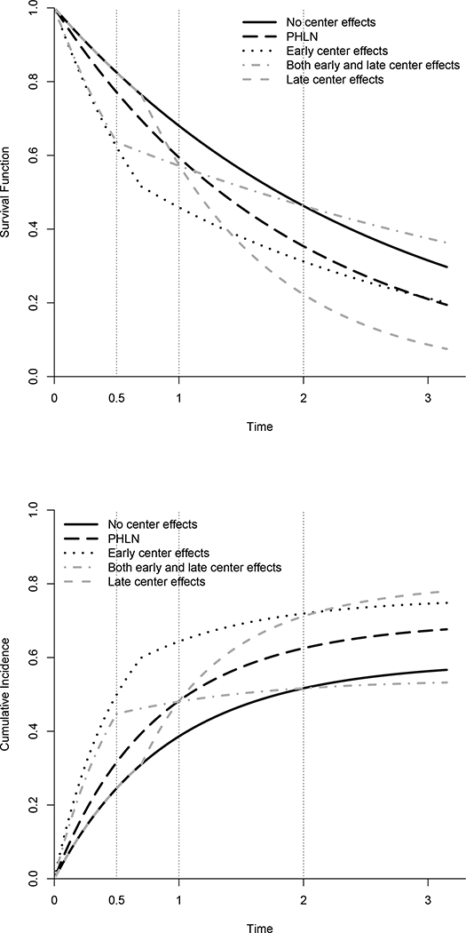
Simulation cenarios for a covariate value of 1. Solid line indicates the null situation, or the curves with a center effect of 0. Other curves represent alternative scenarios at a 1 SD center effect. Upper panel shows the survival curves, while lower panel shows the cumulative incidence curves. Vertical dotted lines represent the time points at which the proposed test is evaluated in the simulations

Table 1.

Type I error rates for survival simulations

K	N	Cluster size / number	Binary covariate				Continuous covariate
			PC(t1)	PC(t2)	PC(t3)	CA	PC(t1)	PC(t2)	PC(t3)	CA
30	450	5/10; 15/10;25/10	0.041	0.039	0.039	0.050	0.040	0.041	0.037	0.050
50	750	5/20;15/20;35/10	0.038	0.037	0.044	0.051	0.039	0.043	0.043	0.052
100	900	3/20;9/40;12/40	0.050	0.051	0.049	0.052	0.049	0.046	0.044	0.048
150	900	3/50;6/50;9/50	0.052	0.050	0.048	0.046	0.051	0.047	0.047	0.045
30	150	1/10;5/10;9/10	0.056	0.039	0.038	0.051	0.055	0.042	0.038	0.047
50	270	l/15;5/15;9/20	0.047	0.041	0.042	0.042	0.049	0.045	0.046	0.050
146	1118	Mimic example	0.041	0.040	0.041	0.049	0.046	0.043	0.040	0.049
30	90	3	0.165	0.061	0.050	0.047	0.160	0.056	0.048	0.045
30	450	15	0.044	0.044	0.042	0.051	0.050	0.042	0.041	0.050
50	150	3	0.106	0.050	0.050	0.042	0.096	0.055	0.053	0.048
50	750	15	0.048	0.048	0.043	0.049	0.045	0.044	0.049	0.052
100	300	3	0.067	0.051	0.048	0.045	0.071	0.058	0.052	0.047
100	900	9	0.049	0.050	0.047	0.049	0.048	0.047	0.050	0.050
150	450	3	0.062	0.051	0.049	0.042	0.062	0.049	0.051	0.044
150	900	6	0.048	0.051	0.051	0.045	0.052	0.051	0.049	0.047

Table 2.

Type I error rates for cumulative incidence simulations

K	N	Cluster size / number	Binary covariate				Continuous covariate
			PC(t1)	PC(t2)	PC(t3)	KB	PC(t1)	PC(t2)	PC(t3)	KB
30	450	5/10; 15/10;25/10	0.035	0.036	0.040	0.034	0.038	0.040	0.039	0.032
50	750	5/20;15/20;35/10	0.041	0.038	0.040	0.034	0.039	0.038	0.038	0.031
100	900	3/20;9/40;12/40	0.046	0.049	0.050	0.029	0.048	0.048	0.049	0.029
150	900	3/50;6/50;9/50	0.049	0.047	0.050	0.029	0.047	0.048	0.045	0.027
30	150	1/10;5/10;9/10	0.041	0.038	0.042	0.033	0.045	0.038	0.038	0.030
50	270	l/15;5/15;9/20	0.047	0.047	0.044	0.033	0.048	0.044	0.044	0.030
146	1118	Mimic example	0.042	0.045	0.040	0.031	0.038	0.040	0.040	0.029
30	90	3	0.090	0.054	0.047	0.035	0.082	0.051	0.044	0.029
30	450	15	0.043	0.042	0.043	0.031	0.046	0.043	0.045	0.036
50	150	3	0.066	0.051	0.050	0.029	0.060	0.049	0.049	0.027
50	750	15	0.042	0.046	0.046	0.030	0.046	0.044	0.047	0.033
100	300	3	0.056	0.050	0.051	0.027	0.056	0.052	0.051	0.028
100	900	9	0.051	0.047	0.047	0.028	0.048	0.048	0.048	0.029
150	450	3	0.055	0.052	0.048	0.023	0.053	0.051	0.052	0.024
150	900	6	0.050	0.049	0.049	0.026	0.049	0.051	0.045	0.026

We can see that in most cases the proposed test controls type I error very well. As the number of clusters increases, the type I error rate is getting close to the nominal level 0.05. The one exception to this is when the cluster size is small (n_k = 3), the type I error is inflated at the early time point. This is likely attributable to the small expected number of events at the early time point. This issue is resolved as the expected number of events increases, either by using a later time point or by increasing the sample size. In additional simulations without censoring (not shown), where pseudo-value regression defaults to generalized linear models for a binary outcome, we have seen similar behavior. This phenomenon does not appear to be attributable to the pseudo-value regression, but rather to the binary outcome modeling with a small number of events. Overall the CA test controls the type I error well since this test uses the entire curve information. The KB test is quite conservative in all the scenarios. We also checked the robustness of the proposed test to misspecificationof the null regression model by conducting a simulation study (not shown) of the performance with an incorrect link function. Our proposed test appeared quite robust to the misspecification of the null regression model through an incorrect link function; however, in general, it is unlikely to be robust against other more severe departures from the null regression model, as the derivation of the null distribution does rely on the correct specification of the null model.

3.2. Power

To study the power of the proposed pseudo-value test, we introduced time dependent random center effects b_k ~ N(0,σ = 0.3) to the proportional hazards or subdistribution hazards model using the following base model

$${\text{λ}}_{kj}\left(t|x_{kj},b_k\right)={\text{λ}}_0(t)\exp \left[x_{kj}\beta +{\gamma }_e{b}_{k}I(t\le t\prime )+{\gamma }_l{b}_{k}I(t>t\prime )\right].$$

Here γ_e denotes the early center effect (prior to time t’) acting on the hazard or subdistribution hazard, while γι denotes the late center effect. While these both act on the hazard function, by choosing different values for γ_e and γ_ι, we can develop models with different net effects on the survival or cumulative incidence at different time points. We considered four specific situations: (i) γ_e = γ_ι, which simplifies to a standard proportional hazards log-normal frailty model (PHLN); (ii) γ_ι = 0, which implies that the center effect only acts on the hazard function at early time points (EARLY); (iii) γ_e = 0, which implies that the center effect only acts on the hazard function at late time points (LATE); and (iv) γ_e > 0 and γι < 0, which implies that the center effect acts in opposition at early versus late time points (BOTH). The cutpoint t’ is chosen to be 0.5 for model (iv) and 0.7 for the other models. For survival data, k₀(t) = λ is assumed constant over time. For competing risks data, the equation above refers to the cause 1 model with the baseline cause 1 subdistribution hazard λ₀(t) satisfying ${\displaystyle {\int }_0^t}{\text{λ}}_0(u)du=\log {[1-p\{1-\exp (-t)\}]}^{-1}$. Then the cause 2 subdistribution hazard is generated according to

$$F_2(t|x_{kj},b_k)=\left[1-F_1\left(\infty |x_{kj},b_k\right)\right]\left[1-\exp \left\{-t\exp \left(x_{kj}\beta +b_k\right)\right\}\right].$$

In order to understand the impact of this time-dependent cluster effect on the parameter being tested (survival or cumulative incidence at a fixed point), plots of the corresponding survival and cumulative incidence curves are shown in Fig. 1. The solid curve is for a center effect of 0 (same for all scenarios), while the other curves represent the various alternative scenarios at a center effect of 1 SD. Vertical lines represent the time points at which the proposed test is evaluated in the simulations.

For the power simulations, a total of 1000 Monte Carlo samples were used. Simulations were also conducted with crossing hazards for the covariate, but the results are similar and so are not shown. The results of the power simulations are shown in Tables 3 and 4 for survival and competing risks respectively.

Table 3.

Power for survival simulations

K	N	Cluster size / number	Model	Binary covariate				Continuous covariate
				PC(t1)	PC(t2)	PC(t3)	CA	PC(t1)	PC(t2)	PC(t3)	CA
50	750	5/20;15/20;35/10	PHLN	0.109	0.221	0.358	0.551	0.125	0.248	0.349	0.542
50	750	5/20;15/20;35/10	Early	0.955	0.918	0.525	0.624	0.962	0.930	0.549	0.639
50	750	5/20;15/20;35/10	Late	0.042	0.301	0.941	0.986	0.041	0.312	0.950	0.983
50	750	5/20;15/20;35/10	Both	0.945	0.297	0.314	0.220	0.947	0.303	0.324	0.221
150	900	3/50;6/50;9/50	PHLN	0.068	0.123	0.180	0.333	0.076	0.115	0.168	0.313
150	900	3/50;6/50;9/50	Early	0.934	0.876	0.296	0.504	0.926	0.852	0.288	0.449
150	900	3/50;6/50;9/50	Late	0.054	0.140	0.874	0.972	0.043	0.163	0.893	0.976
150	900	3/50;6/50;9/50	Both	0.897	0.174	0.194	0.163	0.891	0.159	0.172	0.131
146	1118	Mimic example	PHLN	0.149	0.276	0.410	0.615	0.158	0.259	0.407	0.602
146	1118	Mimic example	Early	0.974	0.945	0.565	0.635	0.976	0.952	0.597	0.672
146	1118	Mimic example	Late	0.044	0.343	0.969	0.994	0.038	0.348	0.962	0.996
146	1118	Mimic example	Both	0.971	0.332	0.362	0.236	0.978	0.336	0.363	0.251
50	750	15	PHLN	0.087	0.158	0.285	0.487	0.092	0.166	0.262	0.481
50	750	15	Early	0.967	0.929	0.451	0.634	0.968	0.921	0.449	0.633
50	750	15	Late	0.042	0.239	0.956	0.993	0.035	0.264	0.946	0.994
50	750	15	Both	0.958	0.249	0.249	0.179	0.957	0.268	0.246	0.185
150	900	6	PHLN	0.073	0.112	0.166	0.287	0.065	0.110	0.166	0.269
150	900	6	Early	0.922	0.853	0.262	0.475	0.921	0.850	0.268	0.447
150	900	6	Late	0.061	0.152	0.856	0.961	0.044	0.125	0.840	0.949
150	900	6	Both	0.846	0.153	0.146	0.109	0.860	0.143	0.142	0.121

Table 4.

Power for cumulative incidence simulations

K	N	Cluster size / number	Model	Binary covariate				Continuous covariate
				PC(t1)	PC(t2)	PC(t3)	KB	PC(t1)	PC(t2)	PC(t3)	KB
50	750	5/20;15/20;35/10	PHLN	0.287	0.445	0.519	0.646	0.318	0.468	0.517	0.650
50	750	5/20;15/20;35/10	Early	0.963	0.942	0.725	0.937	0.954	0.930	0.708	0.933
50	750	5/20;15/20;35/10	Late	0.050	0.385	0.918	0.818	0.034	0.387	0.917	0.821
50	750	5/20;15/20;35/10	Both	0.992	0.861	0.954	0.893	0.992	0.846	0.938	0.891
150	900	3/50;6/50;9/50	PHLN	0.134	0.230	0.294	0.383	0.138	0.217	0.287	0.392
150	900	3/50;6/50;9/50	Early	1.000	0.996	0.877	0.997	0.940	0.879	0.510	0.919
150	900	3/50;6/50;9/50	Late	0.054	0.216	0.832	0.576	0.057	0.221	0.837	0.592
150	900	3/50;6/50;9/50	Both	0.985	0.802	0.941	0.791	0.992	0.803	0.940	0.766
146	1118	Mimic example	PHLN	0.318	0.474	0.567	0.711	0.316	0.477	0.576	0.729
146	1118	Mimic example	Early	0.988	0.952	0.745	0.972	0.984	0.958	0.736	0.978
146	1118	Mimic example	Late	0.041	0.409	0.945	0.870	0.044	0.408	0.942	0.849
146	1118	Mimic example	Both	0.995	0.921	0.973	0.932	0.995	0.913	0.977	0.944
50	750	15	PHLN	0.222	0.341	0.429	0.576	0.195	0.363	0.425	0.591
50	750	15	Early	0.971	0.947	0.652	0.946	0.970	0.958	0.653	0.952
50	750	15	Late	0.045	0.339	0.923	0.787	0.040	0.343	0.922	0.764
50	750	15	Both	0.992	0.877	0.975	0.894	0.995	0.907	0.975	0.904
150	900	6	PHLN	0.136	0.224	0.262	0.373	0.128	0.194	0.253	0.341
150	900	6	Early	1.000	0.996	0.865	0.999	0.909	0.827	0.419	0.870
150	900	6	Late	0.059	0.199	0.801	0.545	0.051	0.203	0.777	0.527
150	900	6	Both	0.973	0.728	0.911	0.695	0.979	0.756	0.912	0.684

For proportional hazards model with a log normal frailty (PHLN), as expected the CA test has the highest power. For the proportional hazards model with an early time dependent random effect (Early), the proposed test has the highest power at time point 1 and second highest power at time point 2, performing much better than the CA test. For the proportional hazards model with a late time dependent random effect (Late), the proposed test has higher power at the late time point only. The CA test has the highest power since it uses the entire curve information. For the crossing hazard model with early and late time dependent random effects in the opposite direction (Both), the proposed test has highest power at the early time point, reflecting the early random effect, but at the later two time points the random effects cancel out.

For the proportional subdistribution hazards model with a log normal frailty model (PHLN), as expected the KB test has the highest power. For the proportional subdistribution hazards model with an early time dependent random effect (Early), the proposed test has the highest power at time point 1 and has better performance than the KB test. For the proportional subdistribution hazards model with late time dependent random effect (Late), the proposed test has the highest power at the late time point and it outperforms the KB test.

For the crossing subdistribution hazards model with early and late time dependent random effects (Both), at the early time point the proposed test has the highest power; at the second time point, the proposed test and KB test have the similar power, and at the late time point the proposed test has higher power than KB test has.

4. Example

In this section, we will illustrate the proposed pairwise correlation pseudo-value test using a retrospective cohort data set from the registry of the Center for International Blood and Marrow Transplant Research (Logan et al. 2011). This cohort includes patients who were receiving a myeloablative HCT from a well matched or partially matched unrelated donor in the years 1995–2004 to treat AML. discussed in the Introduction, many transplant studies are complicated by nonproportional hazards due to the many causes of failure. Our analysis of this dataset is motivated by interest in whether the center effect impacts short term outcomes typically representing direct complications of HCT, as well as long-term prognosis in terms of disease cure. Plots of overall survival and TRM are shown in Fig. 2 to illustrate the early occurrence of TRM as well as the plateau in the survival curve indicating long-term cure. For short-term outcome, we model day 100 TRM (with disease relapse as a competing event) and day 100 survival, and for long-term outcome, we model 2 years survival. Since the patient often stays in the hospital or has frequent contact and access to the hospital in the immediate post transplant period, one might expect a center effect on early outcomes. However, it is less clear whether center practices impact long-term prognosis because of the impact of disease relapse which may be less sensitive to center practices.

Fig. 2.

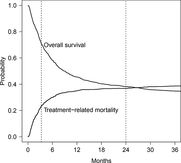
Overall survival and treatment-related mortality for example. The first vertical dotted line represents the time point day 100; the second dotted line represents the time point 2 years

This data set included 1118 patients from 146 transplant centers. Among these patients in terms of overall survival, there were 756 deaths and 362 censored individuals. In terms of TRM, there were 443 TRM events, 328 relapse, and 347 censored individuals. Treatment-related factors include the conditioning regimen (Busulfan + Cyclophosphamide versus Cyclophosphamide + total body irradiation), the graft type (peripheral blood versus bone marrow), the use of graft-versus-host-disease prophylaxis at transplant (CSA + MTX versus CSA [no MTX] versus FK-506 based versus T-cell depletion). Patient- and donor-related factors are age at transplant, disease status prior to conditioning, the cytogenetics risk group, Karnofksy Performance Score (KPS), presence of coexisting disease, and the quality of the HLA match between donor and patient.

A special feature of this data is that center-related factors vary substantially from center to center. The number of patients per center ranges from as few as 1 to as large as 73, with half of the centers having 2–9 patients. Some centers only used one conditioning regimen Cy + TBI, while most of the others only used another conditioning regimen Bu + Cy. Centers also show a strong preference for graft type, using either peripheral blood or bone marrow consistently for almost all of their patients. Given the practice of centers are so different, we are interested in whether the center effects are present so that we can accurately assess the effect of these treatment factors in the presence of center effects.

To test for a potential center effect, we applied the proposed test (at 100 days and 2 years) and the CA test for the survival outcome, while we applied the proposed test (at 100 days) and KB test for the TRM outcome. There is not a significant center effect on the hazard of overall survival using the CA test (p = 0.139), while our proposed test detects a significant center effect on the probability of overall survival at 100 days (p = 0.001) and 2 years (p < 0.001). As mentioned above, center effects may act on different types of events (early transplant-related complications, or disease relapse), and the potential for nonproportional hazards or center effects which are not acting multiplicatively on the hazard function at all time points may make the CA test less sensitive to these center effects. In terms of the center effect on TRM, there is a significant center effect on the subdistribution hazard of overall survival using the KB test (p < 0.001). The proposed test also detects the significant center effect on the cumulative incidence of TRM at 100 days (p = 0.001). These results are consistent with expectations that center practices and close monitoring in the early post-transplant period are likely to impact early transplant-related mortality. In this case, both the proposed test and the KB test give consistent results, likely because there are few additional TRM events beyond 100 days, and the likelihood for nonproportional hazards for TRM within 100 days is less of a concern. We included a scenario that matched our example (denoted “Mimic example” under Cluster size/number column) in the simulation study. For type I error, we can see from Tables 1 and 2, for both survival and cumulative incidence simulations, the mimic example setting had well controlled type I error at each time point. In terms of power, the mimic example setting had exactly the same pattern as all other simulation setting. Therefore, we expect that the proposed test has good performance in the real example.

Since our proposed test is indicating that there are important center effects on both early transplant-related mortality as well as late survival, we further examined the impact of accounting for these center effects in a prognostic factor model. We fit marginal models with and without accounting for clustering using pseudo-values (Logan et al. 2011) to both the 100 day TRM as well as the 2 year survival. The results are in Table 5. Patient and disease characteristics were only included if p < 0.1, while all treatment characteristics (Graft type, conditioning regimen, and GVHD Prophylaxis) were forced into the model. Treatment characteristics are likely to be related to center preferences; hence one might expect that the presence of a center effect would inflate the variance. This is confirmed by noting the SE for treatment factors for the adjusted models are typically around 10–20% higher than for the unadjusted model.

Table 5.

Marginal model results with and without adjustment for center

Outcome	Variable	Comparison	Estimate	Adjusted SE	Unadjusted SE	SE ratio
TRM at 100d	KPS	< 90 vs. >=90	0.243	0.148	0.155	0.954
	Coexisting Dz	Yes vs. No	0.384	0.175	0.158	1.104
	Year	2000–2004 vs. 1995–1999	−0.483	0.183	0.173	1.061
	Graft type	PB vs. BM	−0.504	0.227	0.210	1.079
	Conditioning	BuCy vs. CyTBI	0.046	0.212	0.159	1.337
	GVHD Prophylaxis	CSA (No MTX) vs. CSA+MTX	0.830	0.364	0.331	1.102
		FK506 based vs. CSA+MTX	−0.101	0.229	0.194	1.183
		TCD vs. CSA+MTX	0.275	0.241	0.217	1.114
OS at 2 yhr	Disease status	CR2 vs. CR1	0.039	0.180	0.186	0.968
		REL1 vs. CR1	0.453	0.188	0.210	0.895
		REL2 vs. CR1	0.925	0.260	0.277	0.939
		PIF vs. CR1	0.326	0.228	0.224	1.020
	KPS	<90 vs. >=90	0.435	0.137	0.147	0.927
	Coexisting Dz	Yes vs. No	0.375	0.144	0.148	0.976
	Year	2000–2004 vs. 1995–1999	−0.413	0.181	0.164	1.105
	Graft type	PB vs. BM	−0.264	0.210	0.187	1.119
	Conditioning	BuCy vs. CyTBI	0.073	0.229	0.147	1.553
	GVHD Prophylaxis	CSA (No MTX) vs. CSA+MTX	0.737	0.339	0.331	1.024
		FK506 based vs. CSA+MTX	0.022	0.199	0.175	1.136
		TCD vs. CSA + MTX	0.296	0.252	0.211	1.193

SE Ratios are generally larger than 1 for treatment covariates including Graft type, Conditioning, and GVHD prophylaxis, which are more likely to be related to center preferences

5. Conclusions

The proposed test for a cluster effect has a number of potential benefits. First, the results of the test can help guide the investigator in conducting subsequent analyses in terms of whether they need to adjust for center effects and whether it is worthwhile to try to further characterize the magnitude and source of such center effects. The proposed method tests for a direct center effect on survival probabilities or cumulative incidence at a fixed time point, rather than indirectly testing this through the hazard function. Our method is the first to do tests of center effects using such a direct modeling approach, and as such there are no directly competing methods. Existing tests for cluster effects (CA, KB) in survival data examine the effect of a cluster on the hazard or subdistribution hazard function instead. Our method predictably performs worse when the cluster effect truly acts multiplicatively on the hazard function, but when the center effect is more complex and time-dependent, our method focuses on the time point of interest and appropriately reflects the center effect impact on the probability of interest. As a result, it may have more power than the CA and KB tests to identify differences at that time point. Our method also has a distinct advantage of improved clinical interpretability in settings where the researcher is focused on survival or cumulative incidence probabilities at a clinically relevant time point rather than hazard functions. This is because it directly matches the test of center effect with the clinically relevant parameter of interest. One example where investigators may be more focused on survival or cumulative incidence at a fixed time point is when nonproportional hazards are present, in which case modeling of hazard functions is more complex and difficult to relate to the survival probabilities of interest to clinicians.

The proposed test statistic is easily implemented in a variety of settings. In each case, the form of the test statistic is the same; all that is needed is to compute the pseudovalues for the parameter of interest. Although we have not formally examined restricted mean survival, pseudo-value regression is straightforward to apply to this setting, and the proposed test should directly extend. Further extensions to testing center effects on state probabilities in multistate models are also possible using pseudo-values, as that was one of the original applications of pseudo-value regression; however the theoretic justification is more difficult. Once the pseudo-values are computed, which can be done using the existing R package pseudo, calculation of the center effect test statistic is the same regardless of the setting. We provide R and C code in the supplementary materials for implementing the pseudo-value cluster effect test once thepseudo-values are computed and the fitted values ${\mu }_{kj}^0$ are estimated from a standard generalized estimating equation package such as geepack in R.

The proposed test performs well in simulation studies across a range of settings. It controls the type I error rate well except in settings where there is a very low expected number of events. The simulation studies show in a variety of time-dependent random effect models that the proposed test can gain more power at the appropriate time point where the random center effect distribution is largest, in contrast with the indirect testing through the hazard function used by the existing methods.

While we have focused on a direct modeling approach to test for a center effect at a particular time point, it may be possible to combine the CA test or KB tests with a landmark approach (VanHouwelingen and Putter 2008, 2015), where observations are censored at the time point of interest. This would help to reduce reliance of these tests on the proportional frailty assumption, by only making this assumption up until the time point of interest. This alternative could be investigated further as an alternative to our proposal.

Once a center effect is identified, marginal models or frailty models for the parameter of interest could be considered, as illustrated in our Example above. However, for direct modeling of survival or cumulative incidence at a fixed time point in the presence of a center effect, only methods for marginal models have been published by Logan et al. (2011). We are currently working on random effect models using pseudo-values for such settings.

Finally, we have focused on a single parameter modeled through the pseudo-value. Often it is of interest to simultaneously model survival or cumulative incidence at several time points through a vector of pseudo-values. Extension of the tests described here would be useful to test simultaneously for a center effect at several time points using a vector of pseudo-values.

Appendix: Asymptotic distribution of the proposed test statistic

Here we assume that the cluster size n_k’s and the covariates vector x_kj belong to a bounded set. We also assume standard regularity conditions on the risk set, namely that there exist functions r^c(s) defined on [0, t] with inf_s∈[0,t] r^c(s) > 0 such that

$$\underset{s\in [0,t]}{\sup }\left|a_n^{-2}{R}^c{}^{(n)}(s)-r^c(s)\right|{\to }_{p}0asn\to \infty ,$$

where R^c(t) denotes the number at risk at time t, {a_n} is a sequence of positive constants.

We derive the asymptotic distribution of the proposed test for the competing risks setting, and note that the survival setting can be obtained as a special case. Before we derive the mean, variance, and distribution of the pseudo-value test under H₀, we first present two Lemmas characterizing regularity conditions on the φ_kj.

Lemma 1

Under H₀, var(φ_kj) is bounded.

Proof of Lemma 1

$$\mathrm{var}({\phi }_{kj})=\mathrm{var}\left\{\frac{{\Delta }_{kj}{N}_{kj}(t)}{G(T_{kj})}\right\}$$ (3)

$$+\mathrm{var}\left\{{\displaystyle {\int }_0^{T_{kj}}}\frac{P(T\le t,ϵ=1|T\ge u)}{G(u)}d{M}_{kj}^c(u)\right\}$$ (4)

$$+2\mathrm{cov}\left\{\frac{{\Delta }_{kj}{N}_{kj}(t)}{G(T_{kj})},{\displaystyle {\int }_0^{T_{kj}}}\frac{P(T\le t,ϵ=1|T\ge u)}{G(u)}d{M}_{kj}^c(u)\right\}.$$ (5)

The term in (3) is bounded since ∆_kj(t)N_kj(t) is either 0 or 1 and 1/G(T_kj) is bounded under the regularity conditions on the risk set. The term in (4) can be written as

$$\begin{array}{l}\mathrm{var}\left\{{\displaystyle {\int }_0^{T_{kj}}}\frac{P(T\le t,ϵ=1|T\ge u)}{G(u)}d{M}_{kj}^c(u)\right\}\\ ={\displaystyle {\int }_0^{T_{kj}}}\frac{{(P(T\le t,ϵ=1|T\ge u))}^2}{G^2(u)}I(T_{kj}\ge u){\text{λ}}^c(u)du\\ \le \frac{1}{G^2(T_{kj})}{\text{Λ}}^c(T_{kj}).\end{array}$$

which is bounded due to the regularity conditions on the risk set.

Finally the term in (5) can be rewritten as

$$\begin{array}{l}\mathrm{E}\left\{\frac{{\text{Δ}}_{kj}{N}_{kj}(t)}{G(T_{kj})}{\displaystyle {\int }_0^{T_{kj}}}\frac{P(T\le t,ϵ=1|T\ge u)}{G(u)}d{M}_{kj}^c(u)\right\}\\ =-\mathrm{E}\{\frac{I(T_{kj}\le t)I(\widetilde{T_{kj}}\le C_{kj})}{G(T_{kj})}\\ {\displaystyle {\int }_0^{T_{kj}}}\frac{P(T\le t,ϵ=1|T\ge u)}{G(u)}I(T_{kj}\ge u){\text{λ}}^c(u)du\}.\end{array}$$ (6)

which is bounded in absolute value by Λ^c(T_kj)/G²(T_kj). Therefore var(φ_kj) is bounded.

The second lemma utilizes Lemma 1 to establish additional regularity conditions used to establish the asymptotic distribution of the proposed test statistic; because the results are straightforward given Lemma 1, it is stated without proof. □

Lemma 2

Defining

$$W_k={\displaystyle \sum _{j=1}^{n_k}}{\displaystyle \sum _{j\prime \ne j}^{n_k}}\left({\phi }_{kj}-{\mu }_{kj}^0\right)\left({\phi }_{kj\prime }-{\mu }_{kj\prime }^0\right),$$

the following conditions hold:

• (a)${\displaystyle {\sum }_{k=1}^{\infty }}\left\{\mathrm{var}(\partial W_k/\partial {\beta }_l)/k^2\right\}<\infty$ ∀ l = 1, . . . , p.
• (b)E{∂²W_k/∂β_l∂β_m} is bounded ∀ l,m = 1,…,p and ∀ k.
• (c)${\displaystyle {\sum }_{k=1}^{\infty }}\left\{\mathrm{var}({\partial }^2{W}_k/\partial {\beta }_l{\beta }_m)/k^2\right\}<\infty$ ∀ l = 1, m = 1,. . . , p.
• (d)${\displaystyle {\sum }_{k=1}^K}{\displaystyle {\int }_{\left|z\right|\ge ϵ}}{z}^{2}d{F}_k\to 0$ where z_k = W_k/I^1/2 with distribution function F_k (Lindeberg’s condition).

Based on the conditions established in Lemmas 1 and 2, we can prove the following theorem on the asymptotic distribution of the score test statistic under H₀.

Theorem

Under H₀ and the regularity conditions described above,

$$\frac{T_{PC}(\widehat{\beta })}{\sqrt{I}}\stackrel{D}{\to }N(0,1),$$

where $\widehat{\beta }$ is a consistent estimator of β under H₀.

Proof

First we show that T_PC is asymptotically equivalent to K^−1/2W, where

$$\begin{array}{l}W={\displaystyle \sum _{k=1}^K}{\displaystyle \sum _{j=1}^{n_k}}{\displaystyle \sum _{j\prime \ne j}^{n_k}{W}_k}.\\ TPC=K^{-1/2}{\displaystyle \sum _{k=1}^K}{\displaystyle \sum _{j=1}^{n_k}}{\displaystyle \sum _{j\prime \ne j}^{n_k}}\left\{{\phi }_{kj}-{\mu }_{kj}^0+O_p(K^{-1/2})\right\}\left\{{\phi }_{kj\prime }-{\mu }_{kj\prime }^0+O_p(K^{-1/2})\right\}\\ =K^{-1/2}W+O_p(1)2K^{-1}{\displaystyle \sum _{k=1}^K(n_k-1)}{\displaystyle \sum _{j=1}^{n_k}}\left({\phi }_{kj}-{\mu }_{kj}^0\right)+O_p\left(K^{-1/2}\right).\end{array}$$

Note that $\mathrm{E}\left\{{\displaystyle {\sum }_{j=1}^{n_k}({\phi }_{kj}-{\mu }_{kj}^0})\right\}=0$. Then by the law of large numbers, since nk is bounded and from Lemma 1 $\mathrm{var}({\phi }_{kj}-{\mu }_{kj}^0)$ is bounded,

$$K^{-1}{\displaystyle \sum _{k=1}^K}{\displaystyle \sum _{j=1}^{n_k}}{\displaystyle \sum _{j\prime \ne j}^{n_k}}\left({\phi }_{kj\prime }-{\mu }_{kj\prime }^0\right)=o_p(1).$$

Therefore we have

$$T_{PC}=K^{-1/2}W+o_p(1),$$

and the two statistics will have the same limiting distribution. The mean of the limiting distribution of K^−1/2W is 0 because under H₀, φ_kj is independent of φ_kj′, so that

$$E(K^{-1/2}W)=K^{-1/2}{\displaystyle \sum _{k=1}^K}{\displaystyle \sum _{j=1}^{n_k}}{\displaystyle \sum _{j\prime \ne j}^{n_k}}E\left({\phi }_{kj}-{\mu }_{kj}^0\right)E\left({\phi }_{k{j}^{{}_{\prime }}}-{\mu }_{k{j}^{{}_{\prime }}}^0\right)=0.$$

To derive the variance of the limiting distribution first note that since φ_kj and φ_kj’ are independent under H₀ for j ≠ j′, $\mathrm{E}[({\phi }_{kj}-{\mu }_{kj}^0)({\phi }_{k{j}^{{}_{\prime }}}-{\mu }_{k{j}^{{}_{\prime }}}^0)]=0$ and

$$\mathrm{cov}\left[\left({\phi }_{kj}-{\mu }_{kj}^0\right)\left({\phi }_{k{j}^{{}_{\prime }}}-{\mu }_{k{j}^{{}_{\prime }}}^0\right),\left({\phi }_{kl}-{\mu }_{kl}^0\right)\left({\phi }_{k{l}^{{}_{\prime }}}-{\mu }_{k{l}^{{}_{\prime }}}^0\right)\right]=0,$$

for (l, l′) ≠ (j, j′). Then

$$\begin{array}{l}\mathrm{var}(K^{-1/2}W)=K^{-1}{\displaystyle \sum _{k=1}^K}{\displaystyle \sum _{j=1}^{n_k}}{\displaystyle \sum _{j\prime \ne j}^{n_k}}\mathrm{var}\left[\left({\phi }_{kj}-{\mu }_{kj}^0\right)\left({\phi }_{kj\prime }-{\mu }_{kj\prime }^0\right)\right]\\ =K^{-1}{\displaystyle \sum _{k=1}^K}{\displaystyle \sum _{j=1}^{n_k}}{\displaystyle \sum _{j\prime \ne j}^{n_k}}\mathrm{E}\left[{\left({\phi }_{kj}-{\mu }_{kj}\right)}^2{\left({\phi }_{kj\prime }-{\mu }_{kj\prime }^0\right)}^2\right]\\ =I.\end{array}$$

Proof of asymptotic normality of the test statistic follows closely the derivation in Jacqmin-Gadda and Commenges applied to W, using the regularity conditions in Lemma 2, and so the details are omitted. □

References

- Andersen PK, Hansen MG, Klein JP (2004) Regression analysis of restricted mean survival time based onpseudo-observations. Lifetime Data Anal 10:335–350. 10.1007/s10985-004-4771-0 [DOI] [PubMed] [Google Scholar]
- Andersen PK, Klein JP, RosthØj S (2003) Generalised linear models for correlated pseudo-observations, with applications to multi-state models. Biometrika 90(1):15–27. 10.1093/biomet/90.1.15 [DOI] [Google Scholar]
- Andersen PK, Perme MP (2010) Pseudo-observations in survival analysis. Stat Methods Med Res 19(1):71–99. 10.1177/0962280209105020 [DOI] [PubMed] [Google Scholar]
- Commenges D, Andersen PK (1995) Score test of homogeneity for survival data. Lifetime Data Anal 1:145–156 [DOI] [PubMed] [Google Scholar]
- Fine JP, Gray RJ (1999) A proportional hazards model for the subdistribution of a competing risk. J Am Stat Assoc 94(446):496–509 [Google Scholar]
- Graw F, Gerds TA, Schumacher M (2009) On pseudo-values for regression analysis in multi-state models. Lifetime Data Anal 15:241–255 [DOI] [PubMed] [Google Scholar]
- Gray RJ (1995) Tests for variation over groups in survival data. J Am Stat Assoc 90:198–203 [Google Scholar]
- Jacqmin-Gadda H, Commenges D (1995) Tests of homogeneity for generalized linear models. J Am Stat Assoc 90:1237–1246 [Google Scholar]
- Katsahian S, Boudreau C (2011) Estimating and testing for center effects in competing risks. Stat Med 30:1608–1617 [DOI] [PubMed] [Google Scholar]
- Klein JP, Andersen PK (2005) Regression modeling of competing risks data based on pseudovalues of the cumulative incidence function. Biometrics 61(1):223–229. 10.1111/j.0006-341X.2005.031209.x [DOI] [PubMed] [Google Scholar]
- Klein JP, Logan RB, Harhoff M, Andersen PK (2007) Analyzing survival curves at a fixed point in time. Stat Med 26:4505–4519. 10.1002/sim.2864 [DOI] [PubMed] [Google Scholar]
- Liang KY (1987) A locally most powerful test for homogeneity with many strata. Biometrika 74(2):259–264. 10.1093/biomet/74.2.259 [DOI] [Google Scholar]
- Lin X (1997) Variance component testing in generalised linear models with random effects. Biometrika 84(2):309–326. 10.1093/biomet/84.2.309 [DOI] [Google Scholar]
- Logan BR, Wang T (2014) Chap 10: Pseudo-value regression models In: Klein JP, van Houwelingen HC, Ibrahim JG, Scheike TH (eds) Handbook of survival analysis. CRC Press, Boca Raton [Google Scholar]
- Logan BR, Zhang MJ, Klein JP (2011) Marginal models for clustered time-to-event data with competing risks using pseudovalues. Biometrics 67:1–7 [DOI] [PMC free article] [PubMed] [Google Scholar]
- Satten GA, Datta S (2001) Inverse-probability-of-censoring weighed average. Am Stat 55:207–210 [DOI] [PMC free article] [PubMed] [Google Scholar]
- Scheike TH, Zhang M-J, Gerds T (2008) Predicting cumulative incidence probability by direct binomial-regression. Biomerika 95:205–220 [Google Scholar]
- VanHouwelingen H, Putter H (2008) Dynamic predicting by landmarking as an alternative for multi-state modeling: an application to acute lymphoid leukemia data. Lifetime Data Anal 14:447–463 [DOI] [PMC free article] [PubMed] [Google Scholar]
- VanHouwelingen H, Putter H (2015) Comparison of stopped cox regression with direct methods such as pseudo-values and binomial regression. Lifetime Data Anal 21:180–196 [DOI] [PubMed] [Google Scholar]
Associated Data
This section collects any data citations, data availability statements, or supplementary materials included in this article.