Duration of a minor epidemic

Abstract

Disease outbreaks in stochastic SIR epidemic models are characterized as either minor or major. When ${\mathrm{ℛ}}_0<1$, all epidemics are minor, whereas if ${\mathrm{ℛ}}_0>1$, they can be minor or major. In 1955, Whittle derived formulas for the probability of a minor or a major epidemic. A minor epidemic is distinguished from a major one in that a minor epidemic is generally of shorter duration and has substantially fewer cases than a major epidemic. In this investigation, analytical formulas are derived that approximate the probability density, the mean, and the higher-order moments for the duration of a minor epidemic. These analytical results are applicable to minor epidemics in stochastic SIR, SIS, and SIRS models with a single infected class. The probability density for minor epidemics in more complex epidemic models can be computed numerically applying multitype branching processes and the backward Kolmogorov differential equations. When ${\mathrm{ℛ}}_0$ is close to one, minor epidemics are more common than major epidemics and their duration is significantly longer than when ${\mathrm{ℛ}}_0\ll 1$ or ${\mathrm{ℛ}}_0\gg 1$.

1. Introduction

Public health intervention and control strategies are designed to shorten the course of an epidemic. This is often achieved through reduction of the basic reproduction number ${\mathrm{ℛ}}_0$ to a value below the critical threshold of one. However, for ${\mathrm{ℛ}}_0$ close to one, the duration of an epidemic is increased. This property is demonstrated in the following study of the duration of minor epidemics in stochastic epidemic models.

It is well-known for deterministic SIR epidemic models that if ${\mathrm{ℛ}}_0<1$, the number of infected cases decreases over time, whereas if ${\mathrm{ℛ}}_0>1$, the number of cases increases. However, the outcome differs in stochastic SIR epidemic models. In 1955 Whittle characterized two different types of epidemics in stochastic SIR models as minor or major (Whittle, 1955). Only minor epidemics occur when ${\mathrm{ℛ}}_0<1$ and either minor or major occur when ${\mathrm{ℛ}}_0>1$. Minor epidemics are distinguished from major ones as generally being of shorter duration and with substantially fewer cases. Whittle derived the well-known formulas ${\left(1/{\mathrm{ℛ}}_0\right)}^i$ for the probability of a minor epidemic and $1-{\left(1/{\mathrm{ℛ}}_0\right)}^i$ for the probability of a major epidemic, given there are initially i infected individuals and ${\mathrm{ℛ}}_0>1$. Analytical expressions for the duration of these minor outbreaks are not well known. In this investigation, analytical formulas are derived that approximate the probability density, the mean, and the higher-order moments for a minor epidemic of continuous-time Markov chain (CTMC) SIR, SIS and SIRS epidemic models. In particular, it is shown that the mean duration T of a minor epidemic given $I\left(0\right)=1$ is

$$\mathbb{E}\left(T\right|T<\infty )=\{\begin{array}{cc}\frac{1}{\gamma }\text{ln}\left(\frac{{\mathrm{ℛ}}_0}{{\mathrm{ℛ}}_0-1}\right),& {\mathrm{ℛ}}_0>1,\\ \frac{1}{\beta }\text{ln}\left(\frac{1}{1-{\mathrm{ℛ}}_0}\right),& {\mathrm{ℛ}}_0<1,\end{array}$$

where β is the transmission rate, γ is the recovery rate, and ${\mathrm{ℛ}}_0=\beta /\gamma$.

The probability of a minor or a major epidemic has been studied in more complex disease settings than the CTMC SIR epidemic model by approximating the dynamics with a simple birth-death process, the backward Kolmogorov differential equations, and a multitype branching process approximation (e.g. Allen, 2015; Allen, 2017; Allen & Lahodny, 2012; Allen & van den Driessche, 2013; Athreya & Ney, 1972; Griffiths, 1972; Griffiths, 1973). The probability estimates are generally better for large population sizes and large values of ${\mathrm{ℛ}}_0$ (e.g. Allen, 2015; Allen, 2017; Allen & Lahodny, 2012; Allen & van den Driessche, 2013). Most theoretical research in stochastic models has focused on the duration of major SIR epidemics and quasistationarity in SIS models when conditioned on nonextinction (e.g. Artalejo, 2012; Daley & Gani, 1999; Hernandez-Ceron, Chavez-Casillas, & Feng, 2015; Hernández-Suárez & Castillo-Chavez, 1999; Kryscio & Lefévre, 1989; Norden, 1982; Nåsell, 1996; Nåsell, 1999; Nåsell, 2001; van Doorn, 1991). In this investigation, the emphasis is on the duration of minor epidemics, conditioned on extinction.

In the following section, the simple birth-death process and branching process theory are used to derive the probability density and analytical formulas for the moments for time to extinction. In Section 3, the results from the simple birth-death process are applied to minor epidemics in CTMC SIR and SIS models. Numerical results show good agreement between the simulations and analytical estimates, given the population size is large. The increase in duration when ${\mathrm{ℛ}}_0$ is close to one is demonstrated in these models and in Section 4 as well for the SEIR model with a latent stage.

2. Simple birth-death process

The simple birth-death process is a well-known approximation for many population processes (see e.g. Allen, 2010; Athreya & Ney, 1972; Bailey, 1975; Daley & Gani, 1999; Novozhilov, Karev, & Koonin, 2006; Sehl, Zhou, Sinsheimer, & Lange, 2011; Whittle, 1955). The mean of the simple birth-death process is an exponential growth model,

$$\frac{dm}{dt}=\left(B-D\right)m\text{,}$$ (1)

where B and D are the per capita birth and death rates, respectively. We summarize briefly the simple birth-death process and the expressions that lead to the probability of extinction and the time to extinction.

Let $X\left(t\right)\in \left\{\mathrm{0,1,2},\dots \right\}$ denote the discrete random variable for the population size in a time-homogeneous process with transition probabilities defined as

$$p_{i,j}(t-s)=\mathrm{\mathbb{P}}(X\left(t\right)=j|X\left(s\right)=i)\text{.}$$

The infinitesimal transition probabilities for a small period of time $\text{Δ}t$ can be expressed as

$$p_{i,j}(\Delta t)=\mathrm{\mathbb{P}}(X(t+\Delta t)=j|X\left(t\right)=i)=\{\begin{array}{cc}Bi\Delta t+o\left(\Delta t\right),& j=i+1,\\ Di\Delta t+o\left(\Delta t\right),& j=i-1,\\ 1-\left(B+D\right)i\Delta t+o\left(\Delta t\right),& j=i,\\ o\left(\Delta t\right),& j\ne i-1,i,i+1.\end{array}$$ (2)

The expressions in (2) lead to the backward Kolmogorov differential equations

$$\frac{d{p}_{i,j}}{dt}=Bi{p}_{i+1,j}+Di{p}_{i-1,j}-\left(B+D\right)i{p}_{i,j}\text{.}$$ (3)

An important assumption in the simple birth-death process is that births and deaths occur independently of each other. Therefore, the probability of extinction at time t beginning from i individuals, $p_{i,0}\left(t\right)$, can be written as ${\left(p_{\mathrm{1,0}}\left(t\right)\right)}^i$. Derivation of the expression for $p_{i,0}\left(t\right)$ follows from generating functions and branching process theory (Athreya & Ney, 1972; Bailey, 1975; Daley & Gani, 1999; Harris, 1963):

$$p_{i,0}\left(t\right)=F_i\left(t;D,B\right)=\{\begin{array}{cc}{\left(\frac{D-D{e}^{\left(D-B\right)t}}{B-D{e}^{\left(D-B\right)t}}\right)}^i,& B\ne D,\\ {\left(\frac{Bt}{1+Bt}\right)}^i,& B=D\text{.}\end{array}$$ (4)

An outline of this derivation is given in Appendix A. The probability of ultimate extinction follows directly from (4):

$${\mathrm{\mathbb{P}}}_{\text{ext}}=\underset{t\to \infty }{\text{lim}}{p}_{i,0}\left(t\right)=\{\begin{array}{cc}{\left(\frac{D}{B}\right)}^i,& B>D,\\ 1,& B\le D\text{.}\end{array}$$

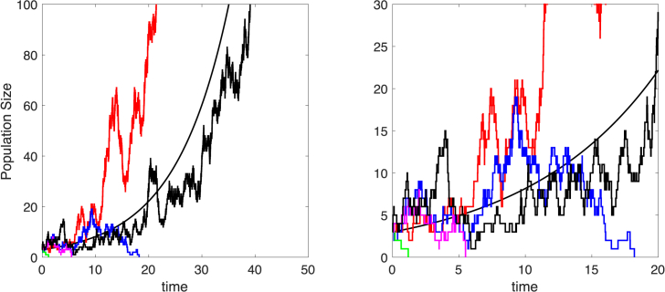
If $B\le D$, extinction occurs with probability one, but if $B>D$, extinction occurs with probability ${\left(D/B\right)}^i$ and the population grows without bound with probability $1-{\left(D/B\right)}^i$. The time to extinction is finite only in the case $B<D$. If $B=D$ the mean time to extinction is infinite while the probability of extinction is one. If $B>D$, the mean time to extinction is also infinite. We are interested in the probability of hitting zero and the time it takes to hit zero, that is, population extinction when $B\ne D$. Therefore, we condition on the time to extinction being finite and only consider those sample paths that hit zero (see Fig. 1).

Fig. 1.

Five sample paths for the simple birth-death process are plotted along with the exponential growth model $m\left(t\right)=3e^{0.1t}$. Three sample paths have finite time to extinction, whereas two sample paths approach infinity. Close-ups of the sample paths are graphed to time 20 on the right. Parameter values are $B=1.1$ and $D=1$, with initial condition $X\left(0\right)=3$. For the simple birth-death process, probability of extinction is ${\mathrm{\mathbb{P}}}_{\text{ext}}={\left(D/B\right)}^3=0.751$ and the mean and the standard deviation for time to extinction, conditioned on extinction, are $\mu =5.34$ and $\sigma =6.71$.

2.1. Probability density function for time to extinction

Let $T_i$ denote the time to extinction given $X\left(0\right)=i$. In the case $B<D$, extinction occurs with probability one, so that the cumulative distribution function (cdf) of $T_i$ is given by $p_{i,0}\left(t\right)=F_i\left(t;D,B\right)$ in (4). In the case $B>D$, extinction occurs with probability ${\left(D/B\right)}^i$. Therefore, conditioned on extinction the cdf of $T_i$ is $p_{i,0}\left(t\right){\left(B/D\right)}^i$. The cdf with $B>D$ is equivalent to the cdf with $B<D$ by interchanging the roles of B and D, i.e., $F_i\left(t;B,D\right)$. Differentiating $F_i$ with respect to t, leads to the pdf for time to extinction:

$$f_{T_i}\left(t\right)=\{\begin{array}{cc}B{\left(1-\frac{D}{B}\right)}^2\frac{i{\rho }_1\left(t\right){\left(1-{\rho }_1\left(t\right)\right)}^{i-1}}{{\left(1-\frac{D}{B}{\rho }_1\left(t\right)\right)}^{i+1}},& B>D,\\ D{\left(1-\frac{B}{D}\right)}^2\frac{i{\rho }_2\left(t\right){\left(1-{\rho }_2\left(t\right)\right)}^{i-1}}{{\left(1-\frac{B}{D}{\rho }_2\left(t\right)\right)}^{i+1}},& B<D,\\ \frac{i{B}^i{t}^{i-1}}{{\left(Bt+1\right)}^{i+1}},& B=D,\end{array}$$ (5)

where ${\rho }_1\left(t\right)=e^{\left(D-B\right)t}$ and ${\rho }_2\left(t\right)=e^{\left(B-D\right)t}$. In the case $B=D$ and $i=1$, $f_{T_1}$ has a Pareto type II distribution (also known as a Lomax distribution) with infinite mean and higher-order moments (Lomax, 1954).

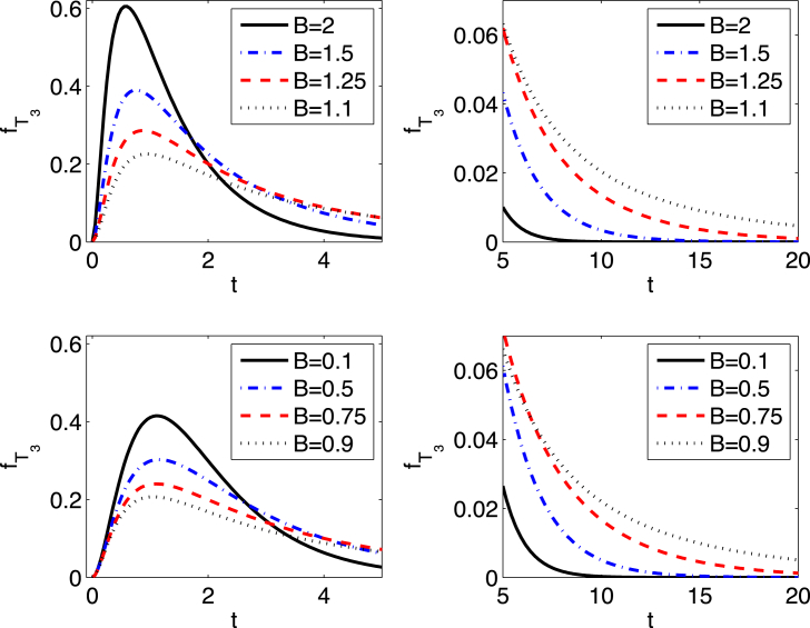
Graphs of the pdf $f_{T_3}$ for parameter values $D=1$, $B>1$ and $B<1$ are plotted for initial conditions $X\left(0\right)=3$ in Fig. 2. The tails of the distribution become “fat” as B approaches one (see Table 1). Some new analytical expressions for the mean and higher-order moments for the time to extinction are computed in the next section.

Fig. 2.

Plots of the pdf $f_{T_3}$ for $D=1$, $B>1$, and $B<1$ show that the tails of the distribution become “fat” as B approaches one.

Table 1.

The probability that time to extinction is greater than five or ten time units given X(0) = 3 and D = 1 (See Fig. 2.).

B	$\mathrm{\mathbb{P}}(T_3>5)$	$\mathrm{\mathbb{P}}(T_3>10)$
2	0.011	6.81$\times {10}^{-5}$
1.5	0.0843	$6.75\times {10}^{-3}$
1.25	0.207	0.0518
1.1	0.325	0.143
0.9	0.347	0.156
0.75	0.249	0.0642
0.5	0.123	0.0101
0.1	0.0297	$3.33\times {10}^{-4}$

2.2. Mean and higher-order moments for time to extinction

The mth moment of $T_i$ can be computed directly from the integral

$$\mathbb{E}\left({\left[T_i\right]}^m\right|T_i<\infty )={\int }_0^{\infty }{t}^m{f}_{T_i}\left(t\right)dt\text{,}$$

where $f_{T_i}\left(t\right)$ is one of the two forms in (5). A closed form analytical expression for the mean when the initial size is $X\left(0\right)=i=1$ is given by

$$\mathbb{E}\left(T_1\right|T_1<\infty )=\{\begin{array}{cc}\frac{1}{D}\text{ln}\left(\frac{B}{B-D}\right),& B>D,\\ \frac{1}{B}\text{ln}\left(\frac{D}{D-B}\right),& B<D\text{.}\end{array}$$ (6)

Karlin and Tavaré (Karlin & Tavaré, 1982) derived the preceding expression in the case $B<D$ when applied to a population genetics model with mutation.

In the following cases, we assume that $D=1$. This assumption is not restrictive since scaling time in (3), $\tau =Dt$, leads to the backward differential equation for $d{p}_{i,j}/d\tau$ expressed in terms of a single parameter $\tilde{B}=B/D$. In the following, we keep the notation B instead of $\tilde{B}$ recalling that $D=1$.

Explicit formulas for the moments are expressed in terms of special functions, polylogarithm functions of order n, ${\text{Li}}_n\left(x\right)$, $n=\mathrm{1,2},\dots$. The polylogarithm function of order n can be expressed as a power series in x (Apostol et al., 2010):

$${\text{Li}}_n\left(x\right)=\sum _{k=1}^{\infty }\frac{x^k}{k^n},0<x<1$$

or defined recursively as

$${\text{Li}}_{n+1}\left(x\right)={\int }_0^x\frac{{\text{Li}}_n\left(t\right)}{t}dt,0<x<1.$$

For order one, the polylogarithm ${\text{Li}}_1$ has a closed form expression, ${\text{Li}}_1\left(x\right)=-\text{ln}\left(1-x\right).$ The first and higher-order moments for the duration until extinction are defined in terms of these special functions.

The mean time to extinction for $D=1$ and $X\left(0\right)=i$ is

$$\mathbb{E}\left(T_i\right|T_i<\infty )=\{\begin{array}{cc}{\text{Li}}_1\left(\frac{1}{B}\right)\sum _{k=1}^i{B}^{k-1}-\sum _{k=1}^{i-1}{H}_k{B}^{k-1},& B>1,\\ {\text{Li}}_1\left(B\right)\sum _{k=1}^i{B}^{k-1-i}-\sum _{k=1}^{i-1}{H}_k{B}^{k-i},& B<1.\end{array}$$ (7)

where $H_j={\sum }_{k=1}^j\left(1/k\right)$ are the harmonic numbers, $H_1=1,H_2=3/2,H_3=11/6$, etc. If the summation is undefined, then it is set to zero. Extensions to higher-order moments when $D=1$ and $X\left(0\right)=i=1$ are

$$\mathbb{E}\left({\left[T_1\right]}^m\right|T_1<\infty )=\{\begin{array}{cc}\frac{m!}{{\left(B-1\right)}^{m-1}}{\text{Li}}_m\left(\frac{1}{B}\right),& B>1,\\ \frac{m!}{B{\left(1-B\right)}^{m-1}}{\text{Li}}_m\left(B\right),& B<1\text{,}\end{array}$$ (8)

for $m=\mathrm{2,3,4},\dots$. The preceding expressions for the moments agree with (6), when $m=1$, $i=1$ and $D=1$.

The higher-order moments $\mathbb{E}\left({\left[T_i\right]}^m\right|T_i<\infty )$, $i>1$, $m>1$ involve several polylogarithm functions. (The explicit expressions for the case $i=2$ and $m>1$ are given in Appendix B.) Recently, Singh et al. (Singh, Schneider, & Myers, 2014) derived formulas for the moments of $T_1$ but for a birth-death process with killing (Karlin & Tavaré, 1982).

The preceding formulas are used to compute some values for the probability of extinction, ${\mathrm{\mathbb{P}}}_{\text{ext}}$, mean $\mu =E\left(T_i\right|T_i<\infty )$, and standard deviation $\sigma ={[\mathbb{E}\left(T_i^2\right|T_i<\infty )-{\mu }_i^2]}^{1/2}$ in Table 2 for $i=3$.

Table 2.

The probability of extinction, the mean, and the standard deviation for the time until extinction, conditioned on extinction, for the simple birth-death process with X(0) = 3 and D = 1.

B	${\mathrm{\mathbb{P}}}_{\text{ext}}$	μ	σ
0.7	1.00	3.50	3.12
0.9	1.00	5.66	6.92
0.95	1.00	7.28	10.93
1.05	0.864	7.05	10.73
1.1	0.751	5.34	6.71
1.5	0.296	2.22	1.92

3. Application to epidemic models

Near the disease-free equilibrium (DFE), the dynamics of the classic differential equations for SIR, SIS, and SIRS epidemics are approximated by the differential equation for infected individuals (Appendix C):

$$\frac{dI\left(t\right)}{dt}=\left(\beta -\gamma \right)I\left(t\right)\text{.}$$

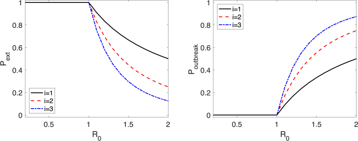
Parameter β is the transmission rate, γ is the recovery rate, and ${\mathrm{ℛ}}_0=\beta /\gamma$. Setting $B=\beta$ and $D=\gamma$, application of the theory from the preceding simple birth-death approximation leads to formulas for the duration of a minor epidemic. It is well-known from Whittle's work in 1955 (Whittle, 1955) that the probability of a minor epidemic, ${\mathrm{\mathbb{P}}}_{\text{ext}}$, or a major epidemic, ${\mathrm{\mathbb{P}}}_{\text{outbreak}}$, given $I\left(0\right)=i$, are

$${\mathrm{\mathbb{P}}}_{\text{ext}}=\{\begin{array}{cc}{\left(\frac{1}{{\mathrm{ℛ}}_0}\right)}^i,& {\mathrm{ℛ}}_0>1,\\ 1,& {\mathrm{ℛ}}_0<1,\end{array}{\mathrm{\mathbb{P}}}_{\text{outbreak}}=\{\begin{array}{cc}1-{\left(\frac{1}{{\mathrm{ℛ}}_0}\right)}^i,& {\mathrm{ℛ}}_0>1,\\ 0,& {\mathrm{ℛ}}_0<1.\end{array}$$ (9)

See Fig. 3. The formulas for the mean and the standard deviation, equations (6), (8), for the duration of a minor epidemic are not well-known:

$$\mathbb{E}\left(T_1\right|T_1<\infty )=\{\begin{array}{cc}\frac{1}{\gamma }\text{ln}\left(\frac{{\mathrm{ℛ}}_0}{{\mathrm{ℛ}}_0-1}\right),& {\mathrm{ℛ}}_0>1,\\ \frac{1}{\beta }\text{ln}\left(\frac{1}{1-{\mathrm{ℛ}}_0}\right),& {\mathrm{ℛ}}_0<1.\end{array}$$ (10)

and for $\gamma =1$,

Fig. 3.

Plot of the probability of a minor outbreak ${\mathrm{\mathbb{P}}}_{\text{ext}}$ and a major outbreak ${\mathrm{\mathbb{P}}}_{\text{outbreak}}$ as a function of ${\mathrm{ℛ}}_0$ for $I\left(0\right)=i$, $i=\mathrm{1,2,3}$.

$$\mathbb{E}\left({\left[T_1\right]}^m\right|T_1<\infty )=\{\begin{array}{cc}\frac{m!}{{\left({\mathrm{ℛ}}_0-1\right)}^{m-1}}{\text{Li}}_m\left(\frac{1}{{\mathrm{ℛ}}_0}\right),& {\mathrm{ℛ}}_0>1,\\ \frac{m!}{{\mathrm{ℛ}}_0{\left(1-{\mathrm{ℛ}}_0\right)}^{m-1}}{\text{Li}}_m\left({\mathrm{ℛ}}_0\right),& {\mathrm{ℛ}}_0<1.\end{array}$$ (11)

In the following sections, for large population sizes, numerical computations for the CTMC SIR ($N=5000$) and CTMC SIS $(N=1000$) models show good agreement with the preceding formulas.

3.1. Stochastic SIR epidemic model

To define the stochastic SIR epidemic model, let $S\left(t\right)$, $I\left(t\right)$, and $R\left(t\right)$ be discrete random variables for the number of susceptible, infected (and infectious), and immune individuals in a homogeneously mixed population with constant total population size N. The CTMC SIR model is a bivariate process that depends on two discrete random variables $S\left(t\right),I\left(t\right)\in \left\{\mathrm{0,1},\dots ,N\right\}$ with transition probabilities,

$$p_{\left(s,i\right),\left(k,j\right)}\left(\Delta t\right)=\{\begin{array}{cc}\beta si\Delta t/N+o\left(\Delta t\right),& \left(k,j\right)=\left(s-1,i+1\right),\\ \gamma i\Delta t+o\left(\Delta t\right),& \left(k,j\right)=\left(s,i-1\right),\\ 1-[\beta si/N+\gamma i]\Delta t+o\left(\Delta t\right),& \left(k,j\right)=\left(s,i\right),\\ o\left(\Delta t\right),& \text{otherwise}.\end{array}$$ (12)

In the following numerical examples, $N=5000$.

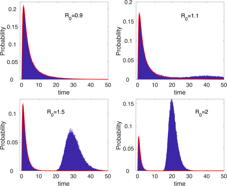
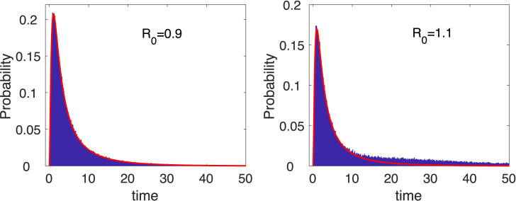
The probability density function for the duration of a minor epidemic in the CTMC SIR epidemic model (12) is plotted as a probability histogram in Fig. 4. All simulations are run until $I\left(t\right)=0$ and the time recorded, $\text{inf}\{t>0|I\left(t\right)=0\}$. The probability histogram shows a mixture of two densities when ${\mathrm{ℛ}}_0>1$: the duration of a minor epidemic with probability ${\mathrm{\mathbb{P}}}_{\text{ext}}$ and the duration of a major outbreak with probability ${\mathrm{\mathbb{P}}}_{\text{outbreak}}$. The density for $f_{T_3}{\mathrm{\mathbb{P}}}_{\text{ext}}$ is the curve overlayed in red on the probability histograms in Fig. 4. The figures illustrate the long duration until disease eradication for ${\mathrm{ℛ}}_0=0.9,1.1$ as opposed to ${\mathrm{ℛ}}_0=1.5,2$.

Fig. 4.

Probability histograms, computed from ${10}^5$ sample paths in the CTMC SIR model (12) show a mixture of two densities when ${\mathrm{ℛ}}_0>1$, the probability of a minor or major epidemic. The curve overlayed in red is a graph of the minor epidemic $f_{T_3}{\mathrm{\mathbb{P}}}_{\text{ext}}$, where $f_{T_3}$ is given in equation (5). Parameter values are $\gamma =1$, $\beta ={\mathrm{ℛ}}_0$, and $N=5000$ with initial conditions $I\left(0\right)=3$, $S\left(0\right)=4997$, and $R\left(0\right)=0$.

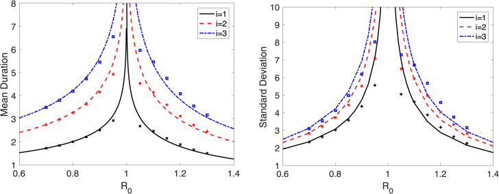
The mean and standard deviation for a minor epidemic are computed numerically in the CTMC SIR model (12) and they are compared to the analytical formulas derived from the simple birth-death process, (10), (11), (20) (Fig. 5). In the numerical simulations of the CTMC SIR epidemic model for ${\mathrm{ℛ}}_0>1$, the sample paths for infected individuals are divided into two sets, those that hit zero before reaching a predefined outbreak level $OL$ (minor epidemic) and those that reach the value $OL$ (major epidemic). The outbreak level is set at $OL=30$. For ${\mathrm{ℛ}}_0<1$, the duration is computed as $\text{inf}\{t>0|I\left(0\right)=i>0\text{and}I\left(t\right)=0\}$ but for ${\mathrm{ℛ}}_0>1$, the duration is $\text{inf}\{t>0|I\left(0\right)=i>0\text{and}I\left(t\right)\notin (0,OL)\}$. If $I\left(t\right)$ hits zero before $OL$, then it is assumed to be a minor epidemic but if $I\left(t\right)$ hits $OL$ before zero, then it is assumed to result in a major epidemic. The values for ${\mathrm{\mathbb{P}}}_{\text{ext}}$, mean, and standard deviation computed from the CTMC SIR simulations and the corresponding approximations from the simple birth-death process are given in Table 3 for the case $I\left(0\right)=3$ in Appendix D.

Fig. 5.

The analytical formulas for the mean and standard deviation, from equations (10), (11), (20) for a minor epidemic are graphed as a function of ${\mathrm{ℛ}}_0$ for three initial conditions $I\left(0\right)=i,i=\mathrm{1,2,3}$. The corresponding mean and standard deviation for duration of a minor epidemic are computed numerically from ${10}^6$ sample paths of the CTMC SIR model (12) (+for $i=1$; x for $i=2$; $\square$ for $i=3$). Parameter values are $\gamma =1$, $\beta ={\mathrm{ℛ}}_0$, and $N=5000$.

3.2. Stochastic SIS model

The dynamics of the CTMC SIS model can be expressed in terms of one discrete random variable $I\left(t\right)\in \left\{\mathrm{0,1},\dots ,N\right\}$, where $s=N-i$.

$$p_{i,j}\left(\Delta t\right)=\{\begin{array}{cc}\beta i\left(N-i\right)\Delta t/N+o\left(\Delta t\right),& j=i+1,\\ \gamma i\Delta t+o\left(\Delta t\right),& j=i-1,\\ 1-[\beta i\left(N-i\right)/N+\gamma i]\Delta t+o\left(\Delta t\right),& j=i,\\ o\left(\Delta t\right),& \text{otherwise}\end{array}.$$ (13)

Numerical computations are performed for the CTMC SIS model (13) similar to those for the CTMC SIR model. The difference is that in the CTMC SIS model when ${\mathrm{ℛ}}_0>1$, all simulations are run until either $I\left(t\right)$ hits zero or $I\left(t\right)$ reaches a predefined outbreak level $OL$. The level $OL$ is either the endemic equilibrium value from the deterministic model: $\overline{I}=N\left(1-1/{\mathrm{ℛ}}_0\right)$ or $OL=30$. In the following numerical examples, $N=1000$.

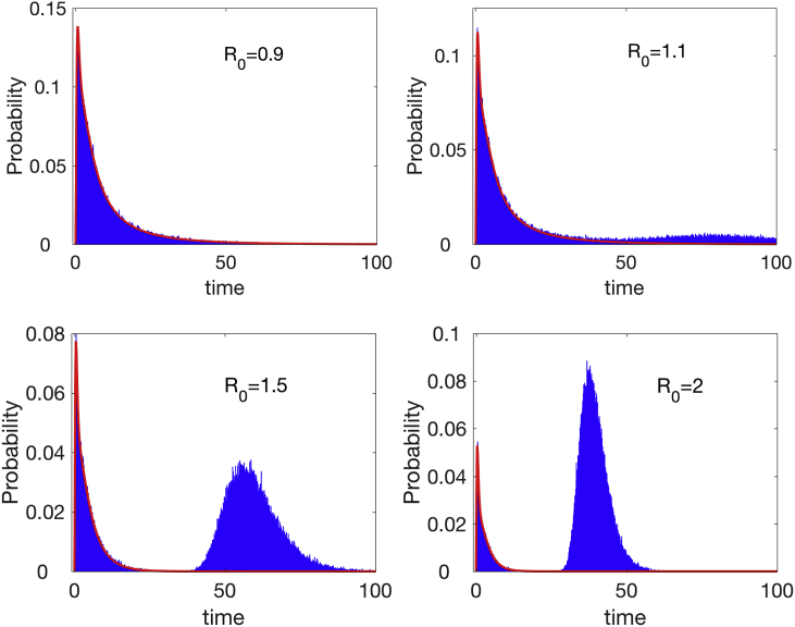
Probability histograms for the duration of minor or major epidemics in the CTMC SIS model (13) are graphed in Fig. 6. For ${\mathrm{ℛ}}_0<1$, the duration of a minor epidemic is $\text{inf}\{t>0|I\left(0\right)=3\text{and}I\left(t\right)=0\}$, whereas for ${\mathrm{ℛ}}_0>1$, the duration is $\text{inf}\{t>0|I\left(0\right)=3\text{and}I\left(t\right)\notin (0,\overline{I})\}$. The curve overlayed in red is the density $f_{T_3}{\mathrm{\mathbb{P}}}_{\text{ext}}$, where $f_{T_3}$ is defined in (5).

Fig. 6.

Probability histograms computed from ${10}^5$ sample paths of the CTMC SIS model show a mixture of two densities when ${\mathrm{ℛ}}_0>1$, the probability of a minor epidemic and the probability of reaching the endemic equilibrium. The overlay curve in red is a graph of $f_{T_3}{\mathrm{\mathbb{P}}}_{\text{ext}}$. Parameter values are $\gamma =1$, $\beta ={\mathrm{ℛ}}_0$ and $N=1000$ with initial conditions $I\left(0\right)=3$ and $S\left(0\right)=997.$

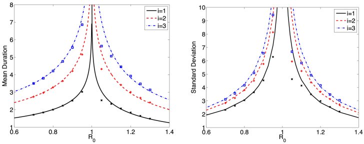
Graphed in Fig. 7 are the mean and standard deviation for duration of a minor epidemic. The curves are from the formulas (10), (11), and (20) in the birth-death process. The calculated values for the CTMC SIS model (12) (similar to Fig. 5) assume a predefined outbreak level of $OL=30$. For ${\mathrm{ℛ}}_0<1$, the duration of a minor epidemic is computed as $\text{inf}\{t>0|I\left(0\right)=i>0\text{and}I\left(t\right)=0\}$ but for ${\mathrm{ℛ}}_0>1$, the duration is computed as $\text{inf}\{t>0|I\left(0\right)=i>0\text{and}I\left(t\right)\notin \left(\mathrm{0,30}\right)\}$. If $I\left(t\right)$ hits 30 before zero, then $I\left(t\right)$ is assumed to reach an endemic level, but if $I\left(t\right)$ hits zero before 30, it is assumed to be a minor epidemic and part of the density $f_{T_i}{\mathrm{\mathbb{P}}}_{\text{ext}}$. Similar to Fig. 5, the numerical values computed for the CTMC SIS model show good agreement with the estimated values from the simple birth-death approximation.

Fig. 7.

The mean and standard deviation, from equations (10), (11), (20), for the time to extinction in the simple birth-death process are graphed as a function of ${\mathrm{ℛ}}_0$ for three initial conditions $I\left(0\right)=i,i=\mathrm{1,2,3}$. Calculated values for the CTMC SIS model (12) are computed from ${10}^6$ sample paths, where the threshold for reaching an endemic equilibrium is set at $OL=30$ (+ for $i=1$, x for $i=2$ and $\square$ for $i=3$). Parameter values are $N=1000$, $\gamma =1$, and $\beta ={\mathrm{ℛ}}_0$.

4. SEIR epidemic model

An SEIR epidemic model includes a latent or an exposed stage, E, where individuals are infected but not yet infectious. The E and I stages in the deterministic model with δ the transition rate from E to I has the form:

$$\begin{array}{l}\frac{dE}{dt}=\beta I\frac{S}{N}-\delta E,\\ \frac{dI}{dt}=\delta E-\gamma I.\end{array}$$

Linearization of this system $\overrightarrow{X}={\left(E,I\right)}^T$ near the DFE, $S\approx N$, yields $d\overrightarrow{X}/dt=\left(F-V\right)\overrightarrow{X}$, where

$$F=\left(\begin{array}{cc}0& \beta \\ 0& 0\end{array}\right)\text{and}V=\left(\begin{array}{cc}\delta & 0\\ -\delta & \gamma \end{array}\right),$$

and ${\mathrm{ℛ}}_0=\rho \left(F{V}^{-1}\right)=\beta /\gamma$ (van den Driessche & Watmough, 2002).

In the corresponding CTMC SEIR model, the transition probabilities include three random variables, $S,E,I$, since $R=N-S-E-I$:

$$p_{\left(s,e,i\right),\left(k,l,m\right)}\left(\text{Δ}t\right)=\{\begin{array}{cc}\beta si\text{Δ}t/N+o\left(\text{Δ}t\right),& \left(k,l,m\right)=\left(s-1,e+1,i\right),\\ \delta e\text{Δ}t+o\left(\text{Δ}t\right),& \left(k,l,m\right)=\left(s,e-1,i+1\right),\\ \gamma i\text{Δ}t+o\left(\text{Δ}t\right),& \left(k,l,m\right)=\left(s,e,i-1\right),\\ 1-[\beta si/N+\delta e+\gamma i]\text{Δ}t+o\left(\text{Δ}t\right),& \left(k,l,m\right)=\left(s,e,i\right),\\ o\left(\text{Δ}t\right),& \text{otherwise}.\end{array}$$ (14)

The multitype branching process approximation is restricted to E and I. The transition probabilities for the branching process are given as (14) but with $s=N$ and

$$p_{\left(e,i\right),\left(l,m\right)}\left(t\right)=\mathrm{\mathbb{P}}((E,I)(t+\text{Δ}t)=(l,m)|(E,I)\left(t\right)=(e,i)).$$ (15)

With no births and deaths, the probability of a minor epidemic is the same as for a CTMC SIR or SIS model, equation (9) and Fig. 3. The parameter δ for transition from exposed to the infectious stage does not affect this probability but does affect the duration of a minor epidemic. Although an analytical formula is not available, the pdf for a minor epidemic can be computed numerically from the solution of the branching process approximation and the backward Kolmogorov differential equations (Appendix E). In Fig. 8, the pdf for the duration a minor or major epidemic are graphed for several values of ${\mathrm{ℛ}}_0$. For ${\mathrm{ℛ}}_0=0.9,1.1$, the duration is much greater as compared to ${\mathrm{ℛ}}_0=1.5,2$ and also, as compared to the CTMC SIR model in Fig. 4. The approximate mean and standard deviation for a minor epidemic are calculated numerically and summarized in Table 5 in Appendix E.

Fig. 8.

Probability histograms, computed from ${10}^5$ sample paths in the CTMC SEIR model show a mixture of two densities when ${\mathrm{ℛ}}_0>1$, the probability of a minor or major epidemic. The curve overlayed in red is a graph of the minor epidemic, computed numerically from the branching process approximation and backward Kolmogorov differential equations in Appendix E. Parameter values are $\gamma =1=\delta$, $\beta ={\mathrm{ℛ}}_0$, and $N=5000$ with initial conditions $I\left(0\right)=3$, $S\left(0\right)=4997$, $E\left(0\right)=0$ and $R\left(0\right)=0$.

5. Conclusion

The birth-death process is well-known in the literature and has been applied to many different biological applications, e.g., (Allen, 2010; Bailey, 1975; Daley & Gani, 1999; Novozhilov et al., 2006; Whittle, 1955). In the birth-death process, either the population size hits zero or approaches infinity. However, conditioned on a finite time to extinction, new analytical formulas are obtained for the mean and higher-order moments for time to extinction when $B/D\ne 1$. These analytical formulas can be applied to stochastic SIS, SIR, and SIRS epidemic models, specifically, formulas (10), (11), (20). For large population sizes, the analytical estimates agree with the simulations from the SIR and SIS epidemic models (Fig. 5, Fig. 7). In addition, minor epidemics play a major role in the dynamics when ${\mathrm{ℛ}}_0$ is close to one (Fig. 4, Fig. 6). The mean duration of a minor epidemic increases when ${\mathrm{ℛ}}_0$ is close to one, as predicted by the analytical formula (10). Additional stages prior to the infected stage, such as a latent stage in the SEIR epidemic model prolong the duration of a minor epidemic (Fig. 8). These results have applications to other infectious disease models and to in-host models (Ciupe & Heffernan, 2017).

Emerging diseases, where the value of ${\mathrm{ℛ}}_0$ is close to one, are likely to have minor epidemics with undetected cases of prolonged duration, allowing time for the pathogen to adapt to the host. This can be of special concern in the case of zoonotic infectious diseases, where the infection may be continually re-introduced into human hosts from animal reservoirs or from an intermediate host (Blumberg & Lloyd-Smith, 2013).

Handling Editor: Jianhong Wu

Appendix.

A Generating Function for Simple Birth-Death Process

The probability generating function (pgf) for the birth-death process $X\left(t\right)$ given $X\left(0\right)=i$ is defined as follows

$$G_i\left(z,t\right)=\mathbb{E}\left(z^{X\left(t\right)}\right|X\left(0\right)=i)=\stackrel{\infty }{\sum _{j=0}}{p}_{i,j}\left(t\right)z^j\text{,}$$ (16)

$$={\left[\mathbb{E}\left(z^{X\left(t\right)}\right|X\left(0\right)=1)\right]}^i={\left[G_1(z,t)\right]}^i\text{,}$$ (17)

where the assumption of independence is applied. Differentiating $G_i$ with respect to t, treating z as constant, applying the relation (17), and equation (3) leads to the differential equation

$$\frac{\partial G_1}{\partial t}=\frac{1}{i{\left(G_1\right)}^{i-1}}\frac{\partial G_i}{\partial t}=\frac{1}{i{G}_{i-1}}\left(\sum _{j=0}^{\infty }\frac{d{p}_{i,j}}{dt}{z}^j\right)\text{.}$$

Substitution of the identify for $d{p}_{i,j}/dt$ from the backward Kolmogorov differential equation (3) leads to

$$\begin{array}{l}\frac{\partial G_1}{\partial t}=\frac{1}{G_{i-1}}\stackrel{\infty }{\sum _{j=0}}\left[p_{i+1,j}B+p_{i-1,j}D-p_{i,j}\left(B+D\right)\right]z^j,\\ =B\frac{G_{i+1}}{G_{i-1}}+D\frac{G_{i-1}}{G_{i-1}}-\left(B+D\right)\frac{G_i}{G_{i-1}},\\ =\left(B+D\right)\left[\frac{B}{B+D}{\left(G_1\right)}^2+\frac{D}{B+D}-G_1\right],\\ =\left(B+D\right)[f\left(G_1\right)-G_1]\text{,}\end{array}$$

where the function f is defined as

$$f\left(u\right)=\frac{B{u}^2+D}{B+D}.$$ (18)

and the initial condition is $G_1\left(z,0\right)=z$.

The expression for f in (18) is the offspring pgf or progeny pgf for the simple birth-death process (Dorman, Sinsheimer, & Lange, 2004; Kimmel & Axelrod, 2002). In a small period of time, each individual either gives birth with probability $B/\left(B+D\right)$ (the individual does not die after giving birth), or dies with probability $D/\left(B+D\right)$. If a birth occurs, the parent is replaced by two individuals (the offspring and the parent). Hence, the probability is multiplied by $u^2$, corresponding to the term $B{u}^2/\left(B+D\right)$ in (18). If a death occurs, the parent dies without any offspring. Hence, the probability is multiplied by $u^0$, corresponding to the term $D/\left(B+D\right)$ in (18).

The solution $G_1\left(z,t\right)$ is well-known (see e.g. (Allen, 2010; Athreya & Ney, 1972; Bailey, 1975),). Applying the relation (17), leads to

$$G_i\left(z,t\right)=\{\begin{array}{cc}{\left(\frac{e^{t\left(D-B\right)}\left(Bz-D\right)-D\left(z-1\right)}{e^{t\left(D-B\right)}\left(Bz-D\right)-B\left(z-1\right)}\right)}^i,& B\ne D.\\ {\left(\frac{1-\left(Bt-1\right)\left(z-1\right)}{1-Bt\left(z-1\right)}\right)}^i,& B=D.\end{array}$$ (19)

Setting $z=0$ in (19) and assuming $p_{\mathrm{1,0}}\left(0\right)=0$ leads to the expression given in (4). The probability of ultimate extinction is the minimal solution of $f\left(q\right)=q$ on $\left[\mathrm{0,1}\right]$. This leads to $q=D/B$, the stable equilibrium solution of $p_{\mathrm{1,0}}$ on $\left[\mathrm{0,1}\right]$ when $B>D$. The only fixed point of f in $\left[\mathrm{0,1}\right]$ is $f\left(1\right)=1$ when $B\le D$.

B Higher-Order Moments in the Birth-Death Process

Analytical expressions for the higher-order moments when $X\left(0\right)=2$ and $D=1$ can be computed with the aid of a computer algebra system. They are expressed in terms of the polylogarithm functions ($m=\mathrm{1,2,3},\dots$):

$$\mathbb{E}\left({\left[T_2\right]}^m\right|T_2<\infty )=\{\begin{array}{cc}\frac{m!}{{\left(B-1\right)}^{m-1}}\left[{\text{Li}}_m\left(\frac{1}{B}\right)\left(B+1\right)-{\text{Li}}_{m-1}\left(\frac{1}{B}\right)\left(B-1\right)\right],& B>1,\\ \frac{m!}{B^2{\left(1-B\right)}^{m-1}}\left[{\text{Li}}_m\left(B\right)\left(B+1\right)-{\text{Li}}_{m-1}\left(B\right)\left(1-B\right)\right],& B<1.\end{array}$$ (20)

C Deterministic SIR, SIS and SIRS Models

The deterministic SIR and SIRS models with transition rate β, recovery rate γ, loss of immunity α, and basic reproduction number ${\mathrm{ℛ}}_0=\beta /\gamma$ are given by the following differential equations:

$$\text{SIS}:\{\begin{array}{c}\frac{dS}{dt}=-\beta I\frac{S}{N}+\gamma I,\\ \frac{dI}{dt}=\beta I\frac{S}{N}-\gamma I,\end{array}\text{SIRS}:\{\begin{array}{c}\frac{dS}{dt}=-\beta I\frac{S}{N}+\alpha R,\\ \frac{dI}{dt}=\beta I\frac{S}{N}-\gamma I,\\ \frac{dR}{dt}=\gamma I-\alpha R.\end{array}$$ (21)

If $\alpha =0$, then the SIRS model simplifies to the SIR model. The total population size is constant, $S\left(t\right)+I\left(t\right)+R\left(t\right)=N$, and initial values are $S\left(0\right)>0$, $I\left(0\right)>0$, and $R\left(0\right)=0$. Near the DFE, $S=N$, $I=0=R$, the dynamics of $I\left(t\right)$ follow an exponential growth model, $dI/dt\approx \left(\beta -\gamma \right)I$.

In the SIR model, $\underset{t\to \infty }{\text{lim}}I\left(t\right)=0$, with an increase in number of infected individuals iff ${\mathrm{ℛ}}_0\left(S\left(0\right)/N\right)>1$. In the SIS model, if ${\mathrm{ℛ}}_0\le 1$, $\underset{t\to \infty }{\text{lim}}I\left(t\right)=0$ and if ${\mathrm{ℛ}}_0>1$, $\underset{t\to \infty }{\text{lim}}I\left(t\right)=N\left(1-1/{\mathrm{ℛ}}_0\right)$. In the SIRS model, if ${\mathrm{ℛ}}_0\le 1$, $\underset{t\to \infty }{\text{lim}}I\left(t\right)=0$ and if ${\mathrm{ℛ}}_0>1$, $\underset{t\to \infty }{\text{lim}}I\left(t\right)=N\left(1-1/{\mathrm{ℛ}}_0\right)\alpha /\left(\alpha +\gamma \right)$.

D CTMC SIR and SIS Simulations

The two tables provide a comparison between the analytical results from the simple birth-death process (${\mathrm{\mathbb{P}}}_{\text{ext}}$, μ, and σ) and the numerical results from the simulations of the CTMC SIR or SIS models (${\mathrm{\mathbb{P}}}_0$, Mean, STD).

Table 3.

Estimates for probability of a minor or major epidemic and the mean and standard deviation for duration of a minor epidemic in the CTMC SIR model (hit zero prior to reaching I(t) = 30), ${\mathrm{\mathbb{P}}}_0$, Mean, and STD, are computed from 10⁶ sample paths. These values are compared to the analytical values ${\mathrm{\mathbb{P}}}_{\text{ext}}$, μ and σ in the birth-death process. Parameters are N = 5000, γ = 1, and $\beta ={\mathrm{ℛ}}_0$ with initial condition I(0) = 3.

${\mathrm{ℛ}}_0$	${\mathrm{\mathbb{P}}}_0$	${\mathrm{\mathbb{P}}}_{\text{ext}}$	Mean	μ	STD	σ
0.7	1	1	3.49	3.50	3.09	3.12
0.75	1	1	3.80	3.82	3.54	3.58
0.8	1	1	4.19	4.23	4.12	4.23
0.85	1	1	4.73	4.80	4.97	5.21
0.9	1	1	5.45	5.66	6.19	6.92
0.95	1	1	6.55	7.28	8.02	10.93
1.05	0.852	0.864	5.96	7.05	7.29	10.73
1.1	0.764	0.751	5.46	5.34	6.70	6.71
1.15	0.674	0.658	4.75	4.42	5.67	5.00
1.2	0.590	0.579	4.08	3.82	4.58	4.03
1.25	0.521	0.512	3.55	3.39	3.75	3.38
1.3	0.462	0.455	3.16	3.05	3.15	2.93

Table 4.

Estimates for probability of a minor epidemic or reaching an endemic level and the mean and standard deviation for duration of a minor epidemic in the CTMC SIS model (hit zero prior to reaching 30), ${\mathrm{\mathbb{P}}}_0$, Mean and STD, are computed from ${10}^6$ sample paths. These values are compared to the analytical values ${\mathrm{\mathbb{P}}}_{\text{ext}}$, μ. and σ in the birth-death process. Parameters are $\gamma =1$ and $\beta ={\mathrm{ℛ}}_0$ with initial condition $I\left(0\right)=3$.

N	$\overline{I}$	${\mathrm{ℛ}}_0$	${\mathrm{\mathbb{P}}}_0$	${\mathrm{\mathbb{P}}}_{\text{ext}}$	Mean	μ	STD	σ
2000	98	1.05	0.833	0.864	5.50	7.05	6.48	10.73
1000	48	1.05	0.840	0.864	5.60	7.05	6.58	10.73
500	24	1.05	0 0.859	0.864	5.88	7.05	7.10	10.73
2000	182	1.1	0.745	0.751	4.94	5.34	5.63	6.71
1000	91	1.1	0.753	0.751	5.08	5.34	5.87	6.71
500	45	1.1	0.772	0.751	5.36	5.34	6.30	6.71
2000	667	1.5	0.298	0.296	2.23	2.22	1.93	1.92
1000	333	1.5	0.300	0.296	2.24	2.22	1.95	1.92
500	167	1.5	0.305	0.296	2.28	2.22	2.00	1.92

E Branching Process Approximation in CTMC SEIR Model

Given the transition probabilities, defined in (15), the generating function for E and I is defined as follows:

$$G_{\left(e,i\right)}\left(z_1,z_2,t\right)=\sum _{l,m}{p}_{\left(e,i\right),\left(l,m\right)}\left(t\right)z_1^l{z}_2^m.$$

Near the DFE, when $S\approx N$ and N is large, the dynamics of E and I can be approximated by a multitype branching process (Allen, 2017; Athreya & Ney, 1972). Assuming independence of E and I,

$$G_{\left(e,i\right)}\left(z_1,z_2,t\right)={\left[G_{\left(\mathrm{1,0}\right)}\left(z_1,z_2,t\right)\right]}^e{\left[G_{\left(\mathrm{0,1}\right)}\left(z_1,z_2,t\right)\right]}^i,$$ (22)

and applying the backward Kolmogorov differential equations,

$$\frac{d{p}_{\left(e,i\right),b}}{dt}=\beta i{p}_{\left(e+1,i\right),b}+\delta e{p}_{\left(e-1,i\right),b}+\gamma i{p}_{\left(e,i-1\right),b}-[\beta i+\delta e+\gamma i]p_{\left(e,i\right),b},$$ (23)

where $b=\left(l,m\right)$, a system of differential equations can be derived for the probability of extinction (Allen, 2017). The derivation is similar to that shown in Appendix A. Differentiation of (22) with respect to t when $\left(e,i\right)=\left(\mathrm{1,0}\right)$ and when $\left(e,i\right)=\left(\mathrm{0,1}\right)$ and application of the backward Kolmogorov differential equation (23) leads to the following differential equations:

$$\begin{array}{l}\frac{\partial G_{\left(\mathrm{1,0}\right)}}{\partial t}=\delta \left[f_1\left(G_{\left(\mathrm{1,0}\right)},G_{\left(\mathrm{0,1}\right)}\right)-G_{\left(\mathrm{1,0}\right)}\right]\\ \frac{\partial G_{\left(\mathrm{0,1}\right)}}{\partial t}=\left(\beta +\gamma \right)\left[f_2\left(G_{\left(\mathrm{1,0}\right)},G_{\left(\mathrm{0,1}\right)}\right)-G_{\left(\mathrm{0,1}\right)}\right],\end{array}$$

where the offspring probability generating functions are

$$\begin{array}{l}{f}_1\left(u_1,u_2\right)=u_2,\\ f_2\left(u_1,u_2\right)=\frac{\beta u_1{u}_2+\gamma }{\beta +\gamma },\end{array}$$

$G_{\left(\mathrm{1,0}\right)}\left(\mathrm{0,0},t\right)=p_{\left(\mathrm{1,0}\right),\left(\mathrm{0,0}\right)}\left(t\right)$, and $G_{\left(\mathrm{0,1}\right)}\left(\mathrm{0,0},t\right)=p_{\left(\mathrm{0,1}\right),\left(\mathrm{0,0}\right)}\left(t\right)$ (Allen, 2017).

The preceding equations are solved numerically and used to compute the pdf for the duration of a minor epidemic (Fig. 8). Computation of the mean μ and standard deviation σ from the pdf gives the approximations in Table 5.

Table 5.

The probability of a minor epidemic and the mean μ and standard deviation σ for the duration of a minor epidemic in the SEIR epidemic given initial conditions $\left(E\left(0\right),I\left(0\right)\right)=\left(\mathrm{0,3}\right)$ or $\left(E\left(0\right),I\left(0\right)\right)=\left(\mathrm{3,0}\right)$ for parameter values $\gamma =1=\delta$ and ${\mathrm{ℛ}}_0=\beta$.

${\mathrm{ℛ}}_0$	${\mathrm{\mathbb{P}}}_{\text{ext}}$	$\left(E\left(0\right),I\left(0\right)\right)=\left(\mathrm{0,3}\right)$		$\left(E\left(0\right),I\left(0\right)\right)=\left(\mathrm{3,0}\right)$
		μ	σ	μ	σ
0.9	1.00	10.48	13.53	11.63	13.47
0.95	1.00	13.82	21.44	14.96	21.38
1.05	0.864	11.82	19.84	12.81	19.80
1.1	0.751	7.84	12.20	8.71	12.20
1.5	0.296	1.325	2.96	1.69	3.25
2	0.125	0.353	1.307	0.517	1.614

References

- Allen L.J.S. 2nd ed. CRC Press; Boca Raton, Fl: 2010. An introduction to stochastic processes with applications to biology. [Google Scholar]
- Allen L.J.S. Springer; 2015. Stochastic population and epidemic models, volume 1.3. Mathematical biosciences lecture series, stochastics in biological systems. [Google Scholar]
- Allen L.J.S. A primer on stochastic epidemic models: Formulation, numerical simulation, and analysis. Infectious Disease Modelling. 2017;2:128–142. doi: 10.1016/j.idm.2017.03.001. [DOI] [PMC free article] [PubMed] [Google Scholar]
- Allen L.J.S., Lahodny G.E., Jr. Extinction thresholds in deterministic and stochastic epidemic models. Journal of Biological Dynamics. 2012;6(2):590–611. doi: 10.1080/17513758.2012.665502. [DOI] [PubMed] [Google Scholar]
- Allen L.J.S., van den Driessche P. Relations between deterministic and stochastic thresholds for disease extinction in continuous-and discrete-time infectious disease models. Mathematical Biosciences. 2013;243(1):99–108. doi: 10.1016/j.mbs.2013.02.006. [DOI] [PubMed] [Google Scholar]
- Apostol T.M. Zeta and related functions. In: Olver F.W.J., Lozier D.W., Boisvert R.F., Clark C.W., editors. NIST handbook of mathematical functions. U.S. Department of Commerce, Cambridge University Press; Cambridge: 2010. pp. 637–650. chapter 10. [Google Scholar]
- Artalejo J.R. On the time to extinction from quasi-stationarity: A unified approach. Physica A: Statistical Mechanics and its Applications. 2012;391(19):4483–4486. [Google Scholar]
- Athreya K.B., Ney P.E. Springer-Verlag; NewYork: 1972. Branching processes. [Google Scholar]
- Bailey N.T.J. Griffin; 1975. The mathematical theory of infectious diseases and its applications. [Google Scholar]
- Blumberg S., Lloyd-Smith J.O. Inference of R0 and transmission heterogeneity from the size distribution of stuttering chains. PLoS Computational Biology. 2013;9(5):e1002993. doi: 10.1371/journal.pcbi.1002993. [DOI] [PMC free article] [PubMed] [Google Scholar]
- Ciupe S.M., Heffernan J.M. In-host modeling. Infectious Disease Modelling. 2017;2:188–202. doi: 10.1016/j.idm.2017.04.002. [DOI] [PMC free article] [PubMed] [Google Scholar]
- Daley D.J., Gani J. Cambridge University Press; Cambridge, U.K: 1999. Epidemic modelling an introduction. [Google Scholar]
- van Doorn E.A. Quasi-stationary distributions and convergence to quasi-stationarity of birth- death processes. Advances in Applied Probability. 1991;23:683–700. [Google Scholar]
- Dorman K.S., Sinsheimer J.S., Lange K. In the garden of branching processes. SIAM Review. 2004;46:202–229. [Google Scholar]
- Griffiths D.A. A bivariate birth-death process which approximates to the spread of disease involving a vector. Journal of Applied Probability. 1972;9(1):65–75. [Google Scholar]
- Griffiths D.A. Multivariate birth-and-death processes as approximations to epidemic processes. Journal of Applied Probability. 1973;10:15–26. [Google Scholar]
- Harris T.E. Springer-Verlag; Berlin: 1963. The theory of branching processes. [Google Scholar]
- Hernandez-Ceron N., Chavez-Casillas J.A., Feng Z. Discrete stochastic metapopulation model with arbitrarily distributed infectious period. Mathematical Biosciences. 2015;261:74–82. doi: 10.1016/j.mbs.2014.12.003. [DOI] [PubMed] [Google Scholar]
- Hernández-Suárez C.M., Castillo-Chavez C. A basic result on the integral for birth-death Markov processes. Mathematical Biosciences. 1999;161(1–2):95–104. doi: 10.1016/s0025-5564(99)00034-6. [DOI] [PubMed] [Google Scholar]
- Karlin S., Tavaré S. Linear birth and death processes with killing. Journal of Applied Probability. 1982;19:477–487. [Google Scholar]
- Kimmel M., Axelrod D.E. Springer; New York: 2002. Branching processes in biology. [Google Scholar]
- Kryscio R.J., Lefévre C. On the extinction of the SIS stochastic logistic epidemic. Journal of Applied Probability. 1989;27:685–694. [Google Scholar]
- Lomax K.S. Business failures: Another example of the analysis of failure data. Journal of the American Statistical Association. 1954;49(268):847–852. [Google Scholar]
- Nåsell I. The quasi-stationary distribution of the closed endemic SIS model. Advances in Applied Probability. 1996;28:895–932. [Google Scholar]
- Nåsell I. On the quasi-stationary distribution of the stochastic logistic epidemic. Mathematical Biosciences. 1999;156:21–40. doi: 10.1016/s0025-5564(98)10059-7. [DOI] [PubMed] [Google Scholar]
- Nåsell I. Extinction and quasi-stationarity in the Verhulst logistic model. Journal of Theoretical Biology. 2001;211:11–27. doi: 10.1006/jtbi.2001.2328. [DOI] [PubMed] [Google Scholar]
- Norden R.H. On the distribution of the time to extinction in the stochastic logistic population model. Advances in Applied Probability. 1982;14(4):687–708. [Google Scholar]
- Novozhilov A.S., Karev G.P., Koonin E.V. Biological applications of the theory of birth-and-death processes. Briefings in Bioinformatics. 2006;7(1):70–85. doi: 10.1093/bib/bbk006. [DOI] [PubMed] [Google Scholar]
- Sehl M.M., Zhou H.H., Sinsheimer J.S., Lange K.L. Extinction models for cancer stem cell therapy. Mathematical Biosciences. 2011;234:132–146. doi: 10.1016/j.mbs.2011.09.005. [DOI] [PMC free article] [PubMed] [Google Scholar]
- Singh S., Schneider D.J., Myers C.R. Using multitype branching processes to quantify statistics of disease outbreaks in zoonotic epidemics. Physical Review E. 2014;89(032702):1–14. doi: 10.1103/PhysRevE.89.032702. [DOI] [PubMed] [Google Scholar]
- van den Driessche P., Watmough J. Reproduction numbers and sub-threshold endemic equilibria for compartmental models of disease transmission. Mathematical Biosciences. 2002;180:29–48. doi: 10.1016/s0025-5564(02)00108-6. [DOI] [PubMed] [Google Scholar]
- Whittle P. The outcome of a stochastic epidemic: A note on Bailey's paper. Biometrika. 1955;42:116–122. [Google Scholar]