Estimation of Spatiotemporal Sensitivity Using Band-limited Signals with No Additional Acquisitions for k–t Parallel Imaging

Abstract

Purpose:

Dynamic MR techniques, such as cardiac cine imaging, benefit from shorter acquisition times. The goal of the present study was to develop a method that achieves short acquisition times, while maintaining a cost-effective reconstruction, for dynamic MRI. k – t sensitivity encoding (SENSE) was identified as the base method to be enhanced meeting these two requirements.

Methods:

The proposed method achieves a reduction in acquisition time by estimating the spatiotemporal (x – f) sensitivity without requiring the acquisition of the alias-free signals, typical of the k – t SENSE technique. The cost-effective reconstruction, in turn, is achieved by a computationally efficient estimation of the x – f sensitivity from the band-limited signals of the aliased inputs. Such band-limited signals are suitable for sensitivity estimation because the strongly aliased signals have been removed.

Results:

For the same reduction factor 4, the net reduction factor 4 for the proposed method was significantly higher than the factor 2.29 achieved by k – t SENSE. The processing time is reduced from 4.1 s for k – t SENSE to 1.7 s for the proposed method. The image quality obtained using the proposed method proved to be superior (mean squared error [MSE] ± standard deviation [SD] = 6.85 ± 2.73) compared to the k – t SENSE case (MSE ± SD = 12.73 ± 3.60) for the vertical long-axis (VLA) view, as well as other views.

Conclusion:

In the present study, k – t SENSE was identified as a suitable base method to be improved achieving both short acquisition times and a cost-effective reconstruction. To enhance these characteristics of base method, a novel implementation is proposed, estimating the x – f sensitivity without the need for an explicit scan of the reference signals. Experimental results showed that the acquisition, computational times and image quality for the proposed method were improved compared to the standard k – t SENSE method.

Introduction

A high acquisition speed is desirable in dynamic MRI, but scanner design, especially for 1.5T systems, often focuses on compactness and energy saving at the expense of hardware performance. In this study, we describe a method that reconciles these requirements, satisfying the following conditions:

1. Shorter acquisition times: Image data should be acquired rapidly within procedurally relevant time to obtain clinically acceptable spatial and temporal resolutions in examinations, such as cardiac cine imaging and dynamic contrast-enhanced myocardial perfusion.

2. Cost-effective reconstruction: Studies focusing on the reduction of acquisition times often rely on reconstruction methods with high-computational costs. However, in the attempt of reducing the cost burden of MRI scanners, a reduction in computational cost is also set as a target for the present study. This condition, on the other hand, cannot impact well understood time limits, defined by the necessity to allow for image review and inspection within the examination time.

In consideration of these primary endpoints, k – t sensitivity encoding (SENSE)¹ was chosen as the base method most suitable for the proposed enhancement. In the following, we first present a novel method for reducing the acquisition time for k – t SENSE, meeting requirement a). While k – t SENSE already achieves requirement b), the presented method further reduces the computational cost.

k – t SENSE

In general, if input signals are undersampled with a regular interval R, the corresponding R signals result being aliased in the Fourier transform. In the transformed data, the spatial distribution of the aliased signals depends on the sampling locations in the signal space.

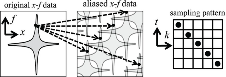
For k – t SENSE, the signal space is referred to as the k – t (k: k-space, t: time) space. The corresponding Fourier-transformed k – t signals are referred to as x – f (x: image, f: frequency) signals. For k – t SENSE, the sampling locations have a regular interval R in both the k-space and time directions and the encoding lines are shifted from one-time frame to the next. As a result, aliasing occurs in the oblique x – f direction (Fig. 1).

Fig. 1.

Aliasing in x – f space. By shifting the sampling pattern in a periodic manner, x – f data are aliased along an oblique x – f direction.

K – t SENSE recovers R signals from the aliased signals by performing the unfold operation in the x – f space. In order to do so, it treats the aliased signals as the weighted sum of the R signals in the x – f space. The weights are referred to as the x – f sensitivity, which is estimated separately through training scans and is therefore assumed to be known in the unfold operation.

Since the main objective of this study is to evaluate the effect of eliminating the training scans, the baseline estimate described in the standard k – t SENSE method was not used.¹ Under this assumption, the R signals ρ can be obtained by solving the following equation:

$$S^{*}{\psi }^{-1}S\rho =S^{*}{\psi }^{-1}{\rho }_{\text{a}}$$ (1)

where S represents the sensitivity matrix for the R aliasing points of all coils, ψ represents the noise covariance matrix for all coils, and ρ_a represents the aliased signals for all coils.

If instead a baseline estimate is available, the equation would need to be slightly modified incorporating the differences between the signals and the baseline estimate. This aspect will not be further investigated in the present study.

While the original k – t SENSE method estimates the R signals by computing a pseudo-inverse matrix, direct solvers (e.g., LU decomposition) can also be used for linear equation systems such as Eq. (1). If a signal term in the vector ρ is known to be zero before solving Eq. (1), the signal and the corresponding elements of the sensitivity matrix can be removed.

x – f sensitivity

The x – f sensitivity is the ratio of the Fourier-transformed coil signals to Fourier-transformed body coil signals. To estimate the x – f sensitivity, alias-free reference signals are needed. Since k – t SENSE undersamples the center of k-space, the sampled signals themselves are not alias-free.

As mentioned above, in the original k – t SENSE, the reference signals are scanned separately. In the alternative SPEAR² method, the signals near the center of the k-space are acquired by dense sampling. In these methods, R_NET, which is the ratio of full-sampled acquisitions to net acquisitions, is less than R. While both these methods provide alias-free signals, the need for additional reference signals comes at the cost of an increased acquisition time.

Methodological benefits

Among the challenges typical of standard k – t SENSE implementations we focused on the following:

1. Unless information concerning the target is incorporated in the method,^3–4 R_NET tends to be much lower than R. For example, in 2D cardiac experiments with k – t SENSE, when R was set to 6, R_NET was 4.6. For example, in 2D cardiac experiments with SPEAR, when R was set to 4, R_NET was 2.9, and when R was set to 8, R_NET was 4.3.

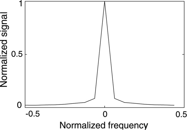
2. The reliability of the x – f sensitivity is assumed to be the same at all frequencies. However, this assumption does not hold. The Fourier transformation of the k – t signals decomposes the average signals of the MR images into direct current (DC) components, and the MR images scatter into non-DC components. In particular for cardiac applications, the DC components correspond to a stationary image that is the average of various cardiac phases. Non-DC signals, conversely, display non-zero values if certain motions, such as heartbeat, are present. Typically, the signal-to-noise ratio (SNR) of DC components is much higher than what displayed by non-DC components (a factor 10 higher in the example shown in Fig. 2).

3. Despite the non-DC signals have a relatively low SNR (Fig. 2), the accuracy of the standard k – t SENSE method decreases as the number of non-DC signals unfolded from an aliased signal increases.

Fig. 2.

Frequency-signal relationship for x – f data with 16 frames. Since the strength of the noise can be considered to be the same at all frequencies, the signal-to-noise ratio (SNR) of the direct current (DC) components is much higher than that of the non-DC components.

The present study proposes a novel method to estimate the x – f sensitivity, and therefore, overcoming the challenges described above. By extending the approach described in an earlier presentation,⁵ instead of using reference signals, the proposed method estimates the x – f sensitivity from the unfolded, undersampled signals, addressing point a). The proposed method then estimates the motion-independent x – f sensitivity from the DC components only, addressing point b). Lastly, the proposed method attempts to detect motion from aliased x – f signals and reduces the number of non-DC components to be unfolded by masking the regions with no signals, accounting for point c).

The concept of the proposed method

For each position x and time t, the image value for coil i can be expressed as

$$I_i(x,t)=(S_i(x)+\Delta S_i(x,t))I(x,t),$$ (2)

where I (x, t) is the image value to be reconstructed, S_i (x) is the motion-independent spatial sensitivity, and ΔS_i (x, t) is the motion-dependent spatial sensitivity. By applying inverse fast Fourier transform (IFFT) (F⁻¹) in the t-direction, the following equation is derived.

$$F^{-1}(I_i(x,t))=S_i(x)F^{-1}(I(x,t))+F^{-1}(\Delta S_i(x,t)I(x,t))$$ (3)

In general, the x – f sensitivity cannot be estimated from the aliased x – f signals without using reference signals. The proposed method obviates to this requirement by approximating the x – f sensitivity with the motion-independent x – f sensitivity and by applying an x – f mask, without requiring the estimation of the non-DC sensitivity term. More in detail, the proposed method assumes that |ΔS_i (x, t)| is small with respect to the motion-independent x – f sensitivity, S_i (x). Under this assumption, the x – f sensitivity is well approximated by S_i (x) because F⁻¹ (I_i(x, t)) ≈ S_i (x) F⁻¹ (I(x, t)).

The premise on |ΔS_i (x, t)| being negligible equates to assuming that no significant movement takes place during image acquisition. In the case of cardiac imaging, this requirement is satisfied by performing acquisitions during breath-holding.

In addition to estimating the motion-independent spatial sensitivity, the proposed method applies an x – f mask identifying the motion-sensitive regions of the x – f sensitivity. The purpose of generating the x – f mask is to identify locations whose signal values are clearly negligible. In order to detect the negligible regions, the proposed method splits the aliased x – f signals into center band signals and non-center band signals. In the center band region, the spatial locations of aliased x – f signals with high signal values identify with the locations to be reconstructed. Conversely, regions for which the x – f signal values are negligible are excluded.

In the non-center band regions, the proposed method attempts to ascertain spatial locations with no motion. This is achieved by identifying the locations in non-center band regions as negligible, when the spatial locations to be reconstructed are masked in the center band region.

The proposed method, thus, extracts band-limited signals (i.e., signals in the center band) and estimates both the sensitivity S_i (x) and x – f mask using the extracted signals. In the band-limited signals, signals aliased strongly are excluded. The signals in non-center bands are not used for estimation of x – f sensitivity.

Materials and Methods

Implementation

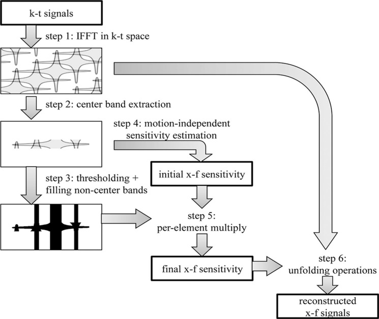
The proposed method, schematically depicted in Fig. 3, requires as inputs the undersampled k – t signals and a threshold for masking, and consists of the following steps:

• Step 1: Application of spatiotemporal IFFT to the input k – t signals. The outputs of this step are aliased x – f signals.

• Step 2: Extraction of the center band for the aliased x – f signals. The outputs of this step are band-limited x – f signals.

• Step 3: Masking of the x – f signal. In the center band, a value of 1 is assigned if the corresponding x – f signal value is above the input threshold, 0 otherwise. In the non-center band region, instead, the mask value is set to 1 where the corresponding f-axis value is above the threshold for both the DC signal and the band-limited part of the non-DC signal, 0 otherwise. The output of this step is the x – f binary mask.

• Step 4: Estimation of the motion-independent sensitivity. For each spatial x position, the sensitivity estimated from the DC component of the aliased x – f signals or one of the aliases is assumed to be motion-independent. The output of this step is the initial x – f sensitivity.

• Step 5: Application of the x – f binary mask to the initial x – f sensitivity. The output of this step is the final x –f sensitivity.

• Step 6: Solution of Eq. (1) with the aliased x – f signals and the x – f sensitivity estimated in the previous steps as inputs. The masked pixels (i.e., with a corresponding value of 0 in the mask) are set to zero and excluded from the pixels to be unfolded. The outputs of this step are the reconstructed x – f signals.

Fig. 3.

Flowchart for the proposed method. The x – f sensitivity is estimated from 1) the x – f signals and 2) the x – f positions where the unfolded values are estimated to be non-zero from the x – f signals. IFFT: inverse fast Fourier transform.

Finally, dynamic images can be reconstructed by applying temporal fast Fourier transform (FFT) to the reconstructed x – f signals.

Evaluation on simulated data

The proposed method was compared with k – t SENSE in a down-sampling simulation to an R-value of 4 using a set of fully-sampled, retrospectively gated cardiac steady-state free precession (SSFP) images. Acquisitions were performed on breath-holding. The DC threshold was set to 4%. The influence of the DC threshold was also evaluated by comparing the results with values of 1%, 10%, and 30%. The non-DC threshold was simply set to 4% in all the experiments. The processing time was measured by running a single-thread C++ implementation on a 2.6-GHz CPU. The performance evaluation was conducted solving Eq. (1) by means of both the standard k – t SENSE and proposed methods.

For the simulation, vertical long-axis (VLA), short-axis (SA), and four-chamber (4ch) views were acquired using a 1.5T scanner. The scanning parameters were 256 readout (RO) steps, 96 phase encode (PE) steps, 15 coil channels, 380 mm × 380 mm FOV of, 8 mm slice thickness of, 4.2 ms TR, 2.1 ms TE, and 40 frames, corresponding to two cardiac cycles. For the k – t SENSE method, 24 reference signals were retained after down-sampling. For each plane, a ROI was drawn for quantitative evaluation. Reconstruction errors were evaluated by computing the frame-by-frame mean squared errors (MSEs) between the fully-sampled and reconstructed images.

In the k – t SENSE case, the simulated acquisition time was 7.1 s (42 × 40 × 4.2 ms); compared to the 4.0 s (24 × 40 × 4.2 ms) simulated acquisition time of the proposed method.

Evaluation on experimental data

In order to evaluate the impact of increasing R-values, k – t signals sampled with R-values of 4, 6, and 8 were acquired and reconstructed using the proposed method. The corresponding number of frames was 12 for an R-value of 4, 18 for an R-value of 6, and 24 for an R-value of 8. Acquisitions were performed on breath-holding. All other scanning parameters matched those used for the simulations.

The acquisition time for each frame was determined by (96 / R) × 4.2 ms, so that the total acquisition time was 1.2 s for each of the R-values (4, 6, and 8).

Results

Evaluation on simulated data

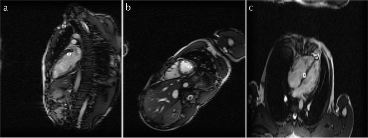
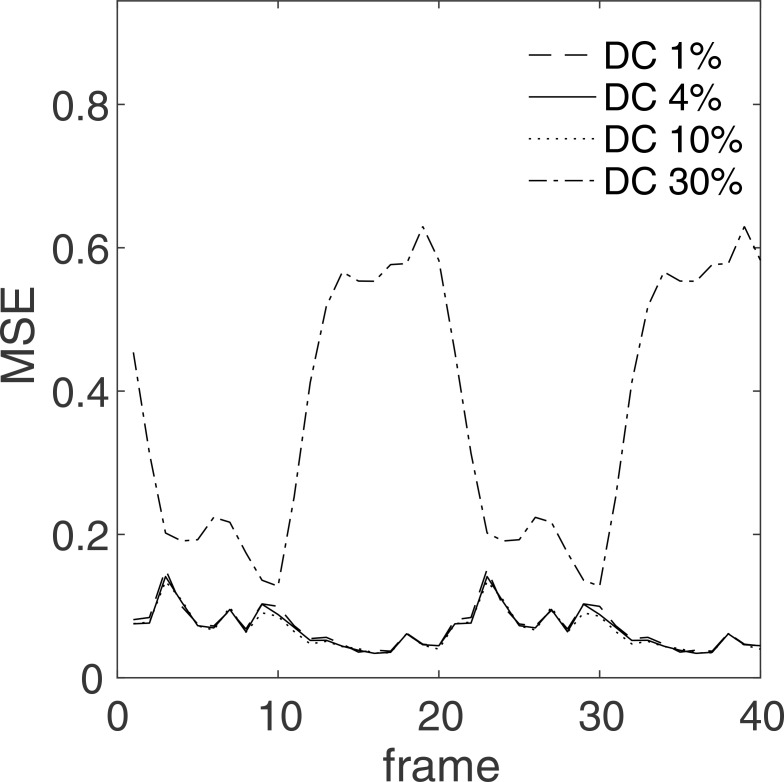
For the ROIs and PE directions shown in Fig. 4, the reconstruction MSEs at different DC thresholds are reported in Table 1 and Fig. 5. As apparent from Fig. 5, the errors are independent of the frame index. When a high threshold is selected, errors are shown increase likely because positions that are critical to the quality of the reconstructed image are being masked. However, as it can be seen in the case of a 1% threshold, a low threshold may also increase the errors (albeit slightly), possibly because it increases the number of positions to be unfolded. In all the simulations considered, the 4% threshold was found to be an acceptable DC threshold.

Fig. 4.

Region of interests for (a) vertical long-axis, (b) short-axis, and (c) four-chamber images. The phase encode directions are horizontal for (a) and vertical for (b and c). The white boxes indicate the ROIs for computing the results shown in Tables 1 and 2.

Table 1.

Reconstruction errors for the proposed method at different direct current (DC) thresholds

DC Threshold Non-DC 4%	VLA Mean ± SD	SA Mean ± SD	4ch Mean ± SD
1%	7.12 ± 2.85	4.60 ± 2.20	8.10 ± 1.98
4%	6.85 ± 2.73	4.46 ± 2.21	7.86 ± 1.77
10%	6.68 ± 2.64	4.46 ± 2.20	19.73 ± 3.43
30%	37.27 ± 18.12	4.46 ± 2.20	39.46 ± 8.70

The table reports the mean and SD for the errors of the proposed method at different DC thresholds calculated on the ROIs shown in Fig. 4 . Higher thresholds can increase the errors, and in all the cases considered, a 4% threshold is found to be an acceptable DC threshold. SA, short-axis; SD, standard deviation; VLA, vertical long-axis; 4ch, four-chamber.

Fig. 5.

Direct current (DC) threshold errors in ROI in the vertical long-axis image. The errors for the ROIs in the remaining images are shown in Table 1. MSE: mean squared error.

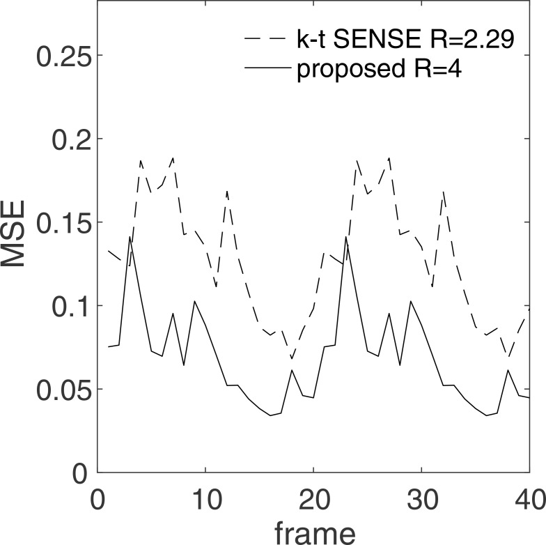
Similarly, the MSEs for k – t SENSE and the proposed method are compared in Table 2, Figs. 6, and 7 for the same ROIs and PE directions. In Table 2 and Fig. 6, the MSEs for the proposed method are shown to be lower than those of k – t SENSE for almost all frames. Additionally, the error images in Fig. 7 display a much lesser conspicuity of bright pixels in the heart region for the proposed method as compared to k – t SENSE.

Table 2.

Comparison of the mean squared errors (MSEs) for x - f sensitivity encoding (SENSE) and the proposed method

Method R = 4	VLA Mean ± SD	SA Mean ± SD	4ch Mean ± SD
k-t SENSE RNET = 2.29	12.73 ± 3.60	7.06 ± 1.80	9.77 ± 2.60
Proposed method RNET = 4	6.85 ± 2.73	4.46 ± 2.21	7.86 ± 1.77

The table reports the mean and standard deviation of the errors for both methods with R = 4 as measured on the ROIs shown in Fig. 4 . The mean errors for the proposed method are lower than those for x – f SENSE. SA, short-axis; SD, standard deviation; LA, vertical long-axis; 4ch, four-chamber.

Fig. 6.

Errors for x – f sensitivity encoding (SENSE) and the proposed method measured on the region of interests drawn on the vertical long-axis image. The errors for the ROIs in the remaining images are shown in Tables 1 and 2. MSE: mean squared error.

Fig. 7.

(a) Image reconstructed using x – f sensitivity encoding (SENSE). (b) Image reconstructed using the proposed method. (c) Error image reconstructed using x – f SENSE. (d) Error image reconstructed using the proposed method. Pixel intensity in (c and d) represents the error between the reconstructed pixel value and the reference pixel value (scaled by 20). White pixels have a high reconstruction error, while black pixels have a low reconstruction error. In the heart region, the error image for the proposed method has a smaller number of white pixels than the error image for x – f SENSE.

Since for the same R the net reduction factor, R_NET, for the proposed method is much higher than the corresponding value for k – t SENSE (Table 2), the proposed method proves to be suitable for fast acquisitions.

The processing time for the VLA image with R = 4 is reported in Table 3. In the sensitivity estimation step, k – t SENSE requires spatial and temporal IFFT for the reference signals. The processing time for IFFT is about 0.8 s. In the unfolding step, the number of locations to be unfolded in k – t SENSE is greater than what required for the proposed method, in which the x – f mask reduces the number of locations to be unfolded. Consequently, the processing time for the proposed method is smaller than what achieved by k – t SENSE.

Table 3.

Processing time (in seconds) for the VLA view with R = 4 for k-t SENSE and the proposed method

Method VLA, R = 4	Sensitivity estimation	Unfolding	FFT in time-axis
k-t SENSE RNET = 2.29	1.69	2.40	0.02
Proposed method RNET = 4	0.25	1.42	0.03

The processing time for the proposed method is smaller compared to k–t SENSE. FFT, fast Fourier transform; SENSE, sensitivity encoding; VLA, vertical long-axis;

Evaluation on experimental data

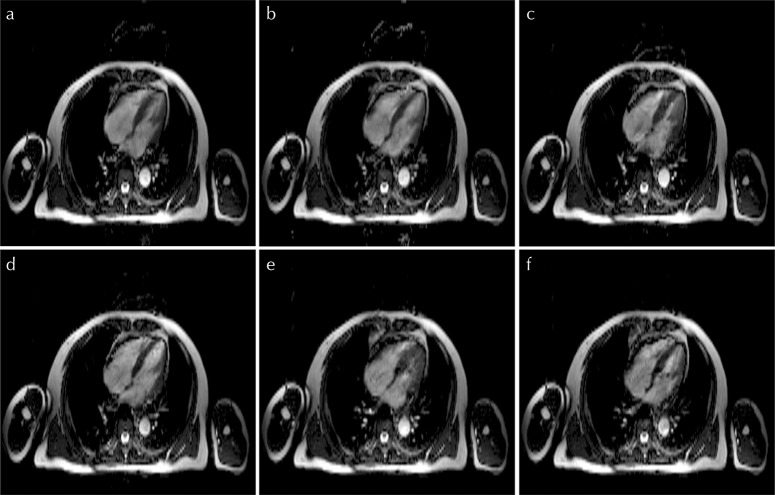
Vertical long-axis and SA reconstructed images with an R_NET value of 8 are shown in Figs. 8 and 9, respectively. Figure 10 shows 4ch reconstructed images with different R_NET values. Artifacts due to aliasing are seen in the 4ch systolic and diastolic views when an R_NET value of 8 is used (Fig. 10). No significant artifacts are seen in any of the VLA and SA images, irrespective of the R-value.

Fig. 8.

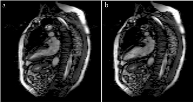
Vertical long-axis images reconstructed using the proposed method with (a and b) R = 8.

Fig. 9.

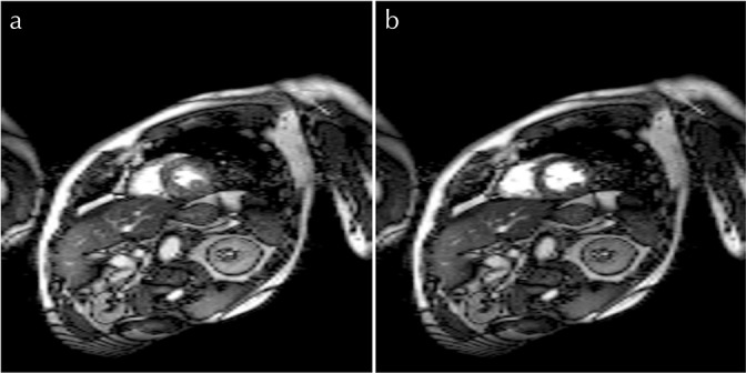
Short-axis (SA) images reconstructed using the proposed method with (a and b) R = 8.

Fig. 10.

Four-chambered images reconstructed using the proposed method with (a and b) R = 4, (c and d) R = 6, and (e and f) R = 8.

For all the R-values, the acquisition time was about 1.2 s per slice. For a single-thread C++ implementation of the proposed method running on a 2.6-GHz CPU, the reconstruction time per slice was 0.78 s for an R-value of 4, 1.09 s for an R-value of 6, and 1.34 s for an R-value of 8. While this reconstruction time is to be considered acceptable for many applications, it can be further improved by algorithm optimization applying methods such as multithreading.

Discussion

Comparison with k – t SENSE

The simulations experiment demonstrated that both the acquisition and computation times for the proposed method were less than what achieved with k – t SENSE. Most relevantly, it was shown that the proposed method increased R_NET, matching R, by estimating the x – f sensitivity without scanning for reference signals or target information. In addition, the simulation also proved that the MSEs for the proposed method are lower than what obtained with k – t SENSE. The proposed method estimates the x – f sensitivity as a countermeasure to the instability of non-DC components: this mechanism is thought to suppress the MSEs associated to the x – f sensitivity instability in k – t SENSE.

The differences in the errors between the two methods, shown in Table 2, are considered to be a result of the differences in the aliased x – f signals in the ROIs. In particular, the mean errors in the VLA image appear to be suppressed because there are no regions characterized by a strong signal along the PE direction from the ROI. This being the case, since the x – f mask removed all the non-DC components in the stationary regions; the number of locations to be unfolded was expected to be reduced to 1 in the proposed method. Conversely, the mean errors for the 4ch image are thought to be higher due to the regions characterized by a strong signal along the PE direction from the ROI.

The experiments proved that an R_NET value of 6 can be achieved with no significant artifacts for the cardiac cine application. However, in order to satisfy the assumption that the subject is stationary, acquisitions are to be performed while breath-holding. If this assumption is not satisfied, i.e., there is significant subject movement during acquisition, the accuracy of the non-DC components of the x – f sensitivity decreases, leading to increases in the errors for the proposed method. While motion correction could be applied to the proposed method, like what was done for k – t SENSE, the computational cost would increase due to alternate, iterated calculations for motion compensation. Relaxation of this assumption is a subject for future work.

The threshold value of 4% used in generating the x – f mask was optimized for the MRI system used in the experiments. The optimal threshold value depends on the amplitude of the noise in the aliased x – f signals. Since the aliased x – f signals are obtained by Fourier transformation of the undersampled k – t signals, the strength of the noise is proportional to the noise in the sampled signals and is inversely proportional to the square root of the number of sampled signals. Since the noise in the sampled signals depends on the particular MRI system in use, tuning is required for each system.

It should be noted that partial Fourier acquisition was not used in this study. The R_NET values can be further improved by applying partial Fourier acquisition and reconstruction, but this would also impact the quality of the reconstructed images.

It was previously shown that optimized sampling patterns are effective in improving the robustness of k – t SENSE.⁷ While the sampling patterns change the oblique direction of aliasing in x – f space, the band-limited x – f signals are not changed much. The proposed method is therefore expected to provide comparable results for optimized sampling patterns.

Though baseline estimation was not used in this study, it can be applied to the proposed method without any restrictions. For applications with longer acquisition times, the acquisition time can be split into fixed lengths and the proposed method can be applied to the k – t signals corresponding to such fixed lengths. In such cases, since the thresholds for the proposed method depend on the length of the acquisition time, the same thresholds can be used even when the acquisition time is split.

Lastly, since the proposed method does not rely on electrocardiogram (ECG) gating, it can be successfully applied to cardiac cine imaging in the presence of irregular heartbeat. On the other hand, the number of PE steps used for the experiments (96 PE steps) was lower than that used in ECG-gated cardiac cine acquisitions (typical, 160 PE steps in a clinical setting⁸). Clinical evaluation of the proposed method remains a subject for future work.

Comparison with other reconstruction methods

When MRI acquisitions are performed with array coils, methods such as parallel imaging (PI), compressed sensing (CS), and low-rank model (LRM) are commonly used to reconstruct highly undersampled data.

Spatial PI methods such as SENSE,⁹ generalized autocalibrating partially parallel acquisitions (GRAPPA),¹⁰ and ESPIRiT¹¹ utilize the differences in receiver coil sensitivities from array coil data. Such methods estimate the sensitivity either by including a separate prescanning step or by employing simultaneous data acquisitions known as autocalibration signals (ACS).

Temporal PI methods such as time-adaptive SENSE (TSENSE)¹² and temporal GRAPPA (TGRAPPA)¹³ estimate the spatial sensitivity from multiple image frames without the acquisition of ACS. For example, TSENSE estimates sensitivity using a temporal low-pass filter, and images are reconstructed using spatial PI (SENSE) and an additional temporal low-pass filter.

Spatiotemporal PI methods assume that images obtained using Fourier transformation in the temporal direction are sparse. Examples of spatiotemporal PI methods are k – t SENSE,¹ SPEAR,² k – t GRAPPA,¹⁴ and k – t principal component analysis (PCA).¹⁵ These methods use spatial and temporal information simultaneously, rather than serially, to achieve high acceleration factors. Spatiotemporal PI methods assume that the subject does not move significantly and require the acquisition of additional information for estimating the spatiotemporal sensitivity.

The CS typically relies on spatial¹⁶ and/or temporal sparseness¹⁷ as L0/L1 cost functions. Low-rank model for dynamic MRI typically exploits temporal image sparseness by representing dynamic pixels as a linear combination of the basis vectors.^18,19 By leveraging the receiver coils sensitivity information, CS/LRM can be combined with PI.

Typically, solvers for CS/LRM iteratively evaluate the consistency between the collected data and prior knowledge. Compressed sensing and its variants require iterative solvers such as iterative shrinkage-thresholding algorithms²⁰ and split Bregman solvers,²¹ at a high computational cost. To reduce the reconstruction time for CS, a graphics processor unit (GPU) implementation has also been evaluated.²² A common LRM solver is a nuclear norm optimizer that uses a scheme such as iterative singular value thresholding. For CS/LRM, an iterative solver such as a conjugate gradient solver is generally used for evaluation of the data consistency of PI.

A comparison of fast acquisition methods is reported in Table 4. While the prior knowledge used in CS/LRM increases the quality of the reconstructed images, the data consistency of PI is evaluated iteratively and several iterations may be required, leading to extremely high computational costs. In contrast, spatial, temporal, and spatiotemporal PI methods rely on L2 cost functions and can therefore be implemented with non-iterative, computationally efficient solvers. Spatiotemporal PI methods, in particular, benefit from both spatial and temporal acceleration, while employing non-iterative solvers. k – t SENSE was therefore found to be a suitable starting technique to implement the novel method evaluated in this work.

Table 4.

Comparison of fast acquisition methods

Method	Spatio-temporal acceleration	Calibration / ACS	Optimization
SENSE	No	Required	L2
GRAPPA	No	Required	L2
TSENSE	Serial	No	L2
TGRAPPA	No	No	L2
k-t BLAST/SENSE	Joint	Required	L2
k-t GRAPPA	Joint	Required	L2
k-t PCA	Joint	Required	L2, PCA
CS (+PI)	Implementation-dependent	No	L0/L1, iterative
LRM (+ PI/CS)	Joint	No	nuclear norm, iterative
Proposed method	Joint	No	L2

Spatiotemporal PI methods enable both spatial and temporal acceleration with non-iterative solvers. ACS, autocalibration signals; BLAST, broad-use linear acquisition speed-up technique; CS, compressed sensing; GRAPPA, GRAPPA, generalized autocalibrating partially parallel acquisitions; LRM, low-rank model; PCA, pontocerebellar angle; PI, parallel imaging; SENSE, sensitivity encoding; TGRAPPA, temporal GRAPPA; TSENSE, encoding incorporating temporal filtering.

Comparison with other calibration methods with no reference signals

Aiming at eliminating the need for explicit scanning of the reference signals, x – f Choice³ uses the characteristics of contrast-enhanced angiography and generates reference signals from the pre-contrast and post-contrast parts of the contrast-enhanced angiography images. A machine-learning approach for eliminating explicit scanning has also been studied.⁴ This method assumes that training data is available for the target organs. However, it is non-trivial to collect training data for the several types of possible lesions.

Non-spatiotemporal PI techniques have also been developed for estimating the sensitivity without explicit information on the target samples. For a radial trajectory, non-Cartesian in nature, the acquired signals near the center of the k-space can be treated as calibration signals.²³ For a Cartesian trajectory, instead, sensitivity can be estimated by LRM in spatial PI.²⁴ However, these methods are not designed for estimation of the x – f sensitivity.

Conclusions

This study aimed at achieving short acquisition times and a cost-effective reconstruction in dynamic MRI acquisitions. After a careful review of existing methods, k – t SENSE was identified as the most suitable reference method for our purpose.

In order to reduce acquisition times as compared to k – t SENSE, a novel method for the estimation of the x – f sensitivity, not requiring explicit scanning of reference signals, was proposed. This method approximates the x – f sensitivity to the motion-independent x – f sensitivity by applying an x – f mask, while the x – f sensitivity and x-f mask are estimated from band-limited x – f signals.

The experimental results showed that the acquisition time, the computational time, and reconstruction errors could be reduced compared to k – t SENSE when applying the proposed method.

References

- 1. Tsao J, Boesiger P, Pruessmann KP. k-t BLAST and k-t SENSE: dynamic MRI with high frame rate exploiting spatiotemporal correlations. Magn Reson Med 2003; 50: 1031– 1042. [DOI] [PubMed] [Google Scholar]
- 2. Xu D, King KF, Liang ZP. Improving k-t SENSE by adaptive regularization. Magn Reson Med 2007; 57: 918– 930. [DOI] [PubMed] [Google Scholar]
- 3. Malik SJ, Schmitz S, O’Regan D, Larkman DJ, Hajnal JV. x-f Choice: reconstruction of undersampled dynamic MRI by data-driven alias rejection applied to contrast-enhanced angiography. Magn Reson Med 2006; 56: 811– 823. [DOI] [PubMed] [Google Scholar]
- 4. Chu ML, Chung HW, Lin YR, Chao TC. Spatiotemporal acceleration of dynamic MR imaging without training data: prior-data-driven k-t PCA. Proceedings of the 20th Annual Meeting of ISMRM, Melbourne, 2012; 2246. [Google Scholar]
- 5. Takeshima H, Nitta S, Shiodera T, Takeguchi T, Yui M, Kuhara S. Method for estimating k-t sensitivity from under-sampled data with no training scans. Proceedings of the 21st Annual Meeting of ISMRM, Salt Lake City, 2013; 3839. [Google Scholar]
- 6. van Amerom JFP, Lloyd DFA, Price AN, et al. Fetal cardiac cine imaging using highly accelerated dynamic MRI with retrospective motion correction and outlier rejection. Magn Reson Med 2018; 79: 327– 338. [DOI] [PMC free article] [PubMed] [Google Scholar]
- 7. Tsao J, Kozerke S, Boesiger P, Pruessmann KP. Optimizing spatiotemporal sampling for k-t BLAST and k-t SENSE: application to high-resolution real-time cardiac steady-state free precession. Magn Reson Med 2005; 53: 1372– 1382. [DOI] [PubMed] [Google Scholar]
- 8. Malayeri AA, Johnson WC, Macedo R, Bathon J, Lima JA, Bluemke DA. Cardiac cine MRI: quantification of the relationship between fast gradient echo and steady-state free precession for determination of myocardial mass and volumes. J Magn Reson Imaging 2008; 28: 60– 66. [DOI] [PMC free article] [PubMed] [Google Scholar]
- 9. Pruessmann KP, Weiger M, Scheidegger MB, Boesiger P. SENSE: sensitivity encoding for fast MRI. Magn Reson Med 1999; 42: 952– 962. [PubMed] [Google Scholar]
- 10. Griswold MA, Jakob PM, Heidemann RM, et al. Generalized autocalibrating partially parallel acquisitions (GRAPPA). Magn Reson Med 2002; 47: 1202– 1210. [DOI] [PubMed] [Google Scholar]
- 11. Uecker M, Lai P, Murphy MJ, et al. ESPIRiT—an eigenvalue approach to autocalibrating parallel MRI: where SENSE meets GRAPPA. Magn Reson Med 2014; 71: 990– 1001. [DOI] [PMC free article] [PubMed] [Google Scholar]
- 12. Kellman P, Epstein FH, McVeigh ER. Adaptive sensitivity encoding incorporating temporal filtering (TSENSE). Magn Reson Med 2001; 45: 846– 852. [DOI] [PubMed] [Google Scholar]
- 13. Breuer FA, Kellman P, Griswold MA, Jakob PM. Dynamic autocalibrated parallel imaging using temporal GRAPPA (TGRAPPA). Magn Reson Med 2005; 53: 981– 985. [DOI] [PubMed] [Google Scholar]
- 14. Huang F, Akao J, Vijayakumar S, Duensing GR, Limkeman M. k-t GRAPPA: a k-space implementation for dynamic MRI with high reduction factor. Magn Reson Med 2005; 54: 1172– 1184. [DOI] [PubMed] [Google Scholar]
- 15. Pedersen H, Kozerke S, Ringgaard S, Nehrke K, Kim WY. k-t PCA: temporally constrained k-t BLAST reconstruction using principal component analysis. Magn Reson Med 2009; 62: 706– 716. [DOI] [PubMed] [Google Scholar]
- 16. Lustig M, Donoho D, Pauly JM. Sparse MRI: the application of compressed sensing for rapid MR imaging. Magn Reson Med 2007; 58: 1182– 1195. [DOI] [PubMed] [Google Scholar]
- 17. Lustig M, Santos J, Donoho DL, Pauly J. k-t SPARSE: high frame rate dynamic MRI exploiting spatio-temporal sparsity. Proceedings of the 14th Scientific Meeting of ISMRM, Seattle, 2006; 2420. [Google Scholar]
- 18. Lingala SG, Hu Y, DiBella E, Jacob M. Accelerated dynamic MRI exploiting sparsity and low-rank structure: k-t SLR. IEEE Trans Med Imag 2011; 30: 1042– 1054. [DOI] [PMC free article] [PubMed] [Google Scholar]
- 19. Otazo R, Candès E, Sodickson DK. Low-rank plus sparse matrix decomposition for accelerated dynamic MRI with separation of background and dynamic components. Magn Reson Med 2015; 73: 1125– 1136. [DOI] [PMC free article] [PubMed] [Google Scholar]
- 20. Beck A, Teboulle M. A fast iterative shrinkage-thresholding algorithm for linear inverse problems. SIAM J Imaging Sci 2009; 2: 183– 202. [Google Scholar]
- 21. Yin W, Osher S, Goldfarb D, Darbon J. Bregman iterative algorithms for ℓ1-minimization with applications to compressed sensing. SIAM J Imaging Sci 2008; 1: 143– 168. [Google Scholar]
- 22. Sabbagh M, Uecker M, Powell AJ, Leeser M, Moghari MH. Cardiac MRI compressed sensing image reconstruction with a graphics processing unit. Proceedings of the 10th International Symposium on Medical Information and Communication Technology (ISMICT), Worcester, 2016; 1– 5. [Google Scholar]
- 23. Arunachalam A, Samsonov A, Block WF. Self-calibrated GRAPPA method for 2D and 3D radial data. Magn Reson Med 2007; 57: 931– 938. [DOI] [PubMed] [Google Scholar]
- 24. Trzasko JD, Manduca A. CLEAR: Calibration-free parallel imaging using locally low-rank encouraging reconstruction. Proceedings of the 20th Annual Meeting of ISMRM, Melbourne, 2012; 517. [Google Scholar]