Abstract
Background
Since task related neurons cannot be specifically targeted during surgery, a critical decision to make is to select which neurons are task-related when performing data analysis. Including neurons unrelated to the task degrades decoding accuracy and confounds neurophysiological results. Traditionally, task-related neurons are selected as those with significant changes in firing rate when a stimulus is applied. However, this assumes that neurons’ encoding of stimuli are dominated by their firing rate with little regard to temporal dynamics.
New Method
This paper proposes a systematic approach for neuron selection, which uses a likelihood ratio test to capture the contribution of stimulus to spiking activity while taking into account task-irrelevant intrinsic dynamics that affect firing rates. This approach is denoted as the model deterioration excluding stimulus (MDES) test.
Results
MDES is compared to firing rate selection in four case studies: a simulation, a decoding example, and two neurophysiology examples.
Comparison with Existing Methods
The MDES rankings in the simulation match closely with ideal rankings, while firing rate rankings are skewed by task-irrelevant parameters. For decoding, 95% accuracy is achieved using the top 8 MDES-ranked neurons, while the top 12 firing-rate ranked neurons are needed. In the neurophysiological examples, MDES matches published results when firing rates do encode salient stimulus information, and uncovers oscillatory modulations in task-related neurons that are not captured when neurons are selected using firing rates.
Conclusions
These case studies illustrate the importance of accounting for intrinsic dynamics when selecting task-related neurons and following the MDES approach accomplishes that. MDES selects neurons that encode task-related information irrespective of these intrinsic dynamics which can bias firing rate based selection.
Keywords: Task-related Neurons, Neuron Selection, Model Based, Point Processes
1. Introduction
Typical neuroscience experiments entail applying a stimulus to a subject and then measuring the brain’s response. Multiple electrodes and microelectrode arrays enable one to record from hundreds of neurons simultaneously during such tasks [1]. However, only some of the neurons may respond to the stimulus. The first and arguably the most critical decision the neuroscientist has to make is to decide which neurons are indeed task-related and which neurons are not prior to data analysis. All the results of these studies are based off this initial decision. Correctly finding these task relevant neurons is important for computational efficiency in these large dimensional spaces as well as for removing noisy channels that may confound results. In some cases, including irrelevant neurons may even drastically change the results leading to incorrect inferences.
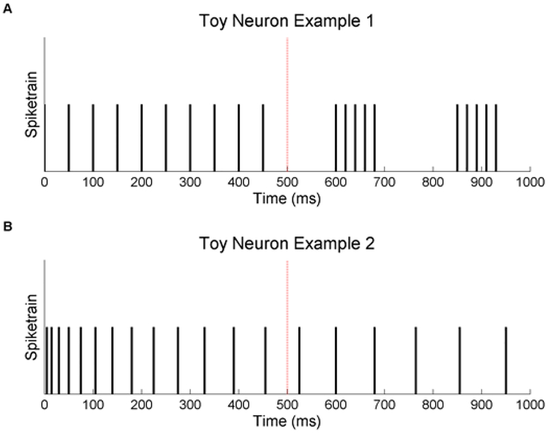
Despite the importance of selecting task-related neurons, the neuroscience community has largely relied on examining changes in firing rates when the stimulus is applied [2–4]. The actual selection at best uses ANOVA analysis of firing rates or at worst is just performed heuristically, which can cause a researcher to be more prone to cherry picking data. When researchers choose by firing rates alone, the implicit assumption is that all of a neuron’s encoding of the stimulus is entailed in its firing rate with no regard for temporal dynamics. At the very least, we know this is false because of a neuron’s refractory period. Figure 1 illustrates two toy examples that further illustrate this point. The spike train in Figure 1A shows an obvious change in temporal dynamics after the stimulus is applied with no change in average firing rate. In contrast the spike train in Figure 1B shows a change in firing rate after the stimulus is applied without any actual change in temporal dynamics. Using firing rate alone in these scenarios could cause task related neurons (Figure 1A) to be excluded from analysis as well as task unrelated neurons (Figure 1B) to be included in analysis. This is not to say that firing rate is not informative, but that the stimulus may be encoded in spike trains in more complicated ways.
Figure 1.
Toy neuron examples show how firing rate can mislabel the task relevance of neurons against a hypothetical stimulus at 500 ms. (A) The first neuron has a change in temporal dynamics to start bursting but has no change in overall firing rate. (B) The second neuron has an decrease in firing rate over time unrelated to the stimulus.
There do exist more powerful methods, such as linear regression analysis or fractional sensitivity analysis. The former uses a linear regression between firing rates and a task relevant parameter, such as direction, but still doesn’t take into account any intrinsic dynamics [2]. The latter bases neuron selection off a neuron’s contribution to decoding the stimulus, which might account for intrinsic dynamics depending on the method of decoding [5]. However, this method only provides relative rankings, does not answer the question of which neurons are task relevant, and also requires a decoding framework, which may not necessarily be available for neurophysiological studies.
In this study, we propose a systematic and theoretically sound approach to selecting task relevant neurons based on the likelihood ratio test, which we call model deterioration excluding stimulus (MDES). For each recorded neuron, we create an encoding model that includes stimulus relevant and irrelevant (e.g. refractory period) parameters that relate to spiking dynamics. We also compute a null model including only the irrelevant parameters. By comparing the performance or more specifically, the likelihood (Equation 1), of the full and the null model using a likelihood ratio test, we can isolate the effects of the stimulus on the neuron’s spiking irrespective of any other dynamics. The larger the increase in likelihood with the addition of the stimulus parameters, the better the neuron is at encoding the stimulus within the model. In essence, with MDES we perform a hypothesis test on whether a neuron’s model performance improves significantly by including task relevant parameters. This is the crux of what researchers seek to achieve when selecting neurons: “Does this neuron significantly encode experimental parameters?” The calculated p-value can be used as a selection criterion useful for neurophysiological studies or as a ranking system useful for decoding applications.
| (1A) |
| (1B) |
We then compare this model-based selection with firing rate ANOVA analysis in 4 cases (1 simulation, 1 decoding, and 2 neurophysiological examples). In the first case, we simulate neurons that have different intrinsic and extrinsic parameters and compare the model-based rankings and firing rate rankings with a predefined ideal ranking. The simulation shows that there can exist intrinsic dynamics in which firing rate rankings become skewed while model-based rankings do not. In the second case, we examine the performance of the best MDES-based neurons to decode dexterous finger movements and compare the results with the performance of the best firing rate ranked neurons [6]. In the last two cases, we observe neurophysiological studies. For the first of these two, we compare action value versus action selection related neurons in prefrontal cortex and striatum neurons [7]. Previous papers have successfully distinguished these populations with firing rate and we show that our model-based selection does not fail where firing rate already works. Finally in the last case, we search in the basal ganglia for oscillatory activity that is indicative of movement planning in only directionally tuned neurons [8]. This oscillatory activity turns out to be more robust in the population selected through our model-based method. All of a study’s inferences rely on the fidelity of the neurons chosen to be analyzed. These cases show that including unrelated neurons and/or excluding relevant neurons can confound and skew results in the form of decoding performance or neurophysiological conclusions. Using MDES as opposed to just firing rates can more rigorously select for these task-related neurons.
2. Methods
2.1. Point Process Model
In each case of the four cases point process modeling (PPM) will be used with generalized linear methods (GLM) to construct encoding models. PPMs can successfully model spike trains as a function of both intrinsic and extrinsic properties in a variety of brain areas [9–22] while the GLM framework provides an efficient computational scheme for parameter estimation [21, 23] with well known statistical bounds [24].
A point process is a series of 0–1 random events that occur in continuous time. For a neural spike train, the 1s are individual spike times and the 0s are the times at which no spikes occur. To define a point-process model of neural spiking activity, consider an observation interval (0, T] and let N(t) be the number of spikes counted in interval (0, t] for t є (0, T]. A point-process model of a neural spike train is then completely characterized by its conditional intensity function (CIF), λ(t|Xt), defined as follows:
| (2) |
where Xt represents a vector of covariates at time interval (t, t + δ]. These covariates can represent intrinsic effects such as spiking history and extrinsic effects such as kinematics or network dynamics. It follows from equation (2) that the probability of a single spike in a small interval (t, t + δ] is approximately
| (3) |
Details can be found in [25] and [28]. When δ is small, equation (2) approximates the spiking propensity at time t. The CIF generalizes the rate function of a Poisson process to a rate function that is dependent on the covariates that can change over time. Because the CIF completely characterizes a spike train, defining a model for the CIF defines a model for the spike train[21, 27].
For our examples, we use the GLM framework to define our CIF models by expressing, for each neuron, the log of its CIF as a linear combination of the covariates [28]. More specifically, log[λ(k|Xt)] = α + βXt where the scalar, α, and the vector, β, represent the parameters being fit. The GLM is an extension of the multiple linear regression model in which the variable being predicted (in this case, spike times) need not be Gaussian [29]. The GLM also provides an efficient computational scheme for estimating model parameters and a likelihood framework for conducting statistical inferences [21].
2.2. Model Deterioration Excluding Stimulus for PPMs
Using a set of spike trains, a full model from equation (1A) is first fitted that contains all the dynamics of the neuron sought to be modeled as log[λfull(t|Xt)] = f(Xstim, Xother). A null model from equation (1B) is separately fitted as log[λreduced(t|Xt)] = f(Xother) without any stimulus parameters. The likelihood of the observed spike trains given the model is calculated as
| (4) |
The MDES statistic follows the likelihood ratio test and is calculated as
| (5) |
It is approximated by the χ2 distribution where the degrees of freedom are equal to the number of parameters lost in the null model. A larger ratio corresponds to a higher task relevance of the neuron. An ordered ranking can be obtained by sorting a group of these test statistics. A division between task relevant and task irrelevant neurons can be obtained by using the χ2 distribution to obtain p-values and selecting an appropriate statistical power (e.g. 5%) using:
| (6) |
where Γ(·) is the gamma function and v represents the degrees of freedom.
3. Results
3.1. Case 1 - Simulation
3.1.1. Experiment
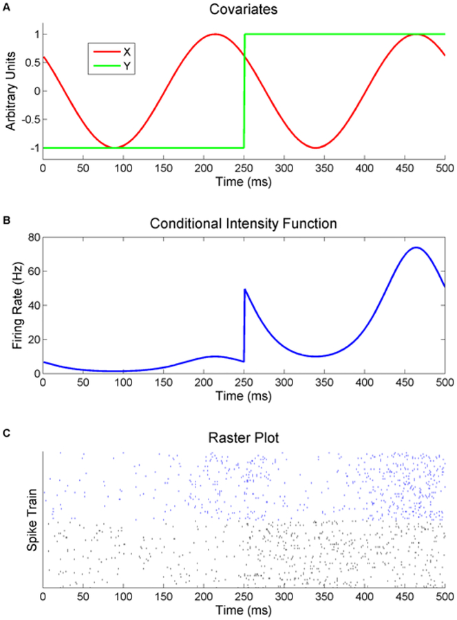
We first simulate neuronal activity in response to a stimulus variable as a function of two covariates, X and Y, as shown in Figure 2A. The stimulus covariate represents the application of an external stimulus such as a go cue for a movement or simply an image presentation for a visual task and is defined as
| (7) |
over a 500 ms trial period where us(t) is the Heavyside step function. The intrinsic covariate represents some oscillating intrinsic activity that is not time locked with the stimulus onset and is defined as
| (8) |
where the frequency, f, is free to be defined and the phase, ϕ, is randomly generated from trial to trial.
Figure 2.
An example of the stimulus related (Y) and unrelated (X) covariates (A, top) as well as the accompanying conditional intensity function (B, middle) for f = 4, exp(α) = 10, β = γ = ϕ = 1. The stimulus covariate represents the onset of some stimulus while the unrelated covariate represents some background intrinsic dynamics. A random phase offset is introduced as the unrelated covariate should not be time synced to the stimulus onset. A raster plot (C, bottom) shows multiple trials of simulated data using this CIF. The top half of the trials (blue) are specifically for ϕ = 1. The bottom half of the trials (black) simulate multiple recordings over time as ϕ varies randomly from trial to trial.
Using this stimulus covariate, Yt, and intrinsic covariate, Xt, a number of neurons are simulated. Neuron spike trains are generated using a bin size of 1 ms with the following CIF:
| (9) |
where β and γ are constant scalars unique to a specific neuron and define how that neuron’s spiking is effected by the two covariates. The basal firing rate is determined by α and is set to log(10) for all simulated neurons. Neurons with β and γ values ranging from 0 to 1.0 and −1.0 to 1.0 respectively are simulated. The parameter values are gridded by 0.1 leading to 231 neurons total for a set intrinsic covariate frequency, f, each with a unique β and γ. Each neuron has 100 trials of 500 ms of data. An example conditional intensity function generated by equation (9) is also shown for the covariates shown in Figure 2B with parameter values of f = 4 Hz, exp(α) = 10, and β = γ = ϕ = 1. Figure 2C then shows a raster plot of example spike trains. The top quarter (blue) shows spike trains from the example CIF and the firing rate visually matches it. The rest of the trials (black) match a more realistic recording scenario where the intrinsic phase would vary randomly from trial to trial.
3.1.2. Model
The full model naturally follows the model used to generate the data while the null model is missing the stimulus covariate:
| (10A) |
| (10B) |
3.1.3. Method of Comparison
Using the 100 trials of spike trains, a full and null model is fitted for each neuron. From this, the MDES statistic is calculated for each neuron. The neurons are then sorted and ranked by this statistic to see which neurons are most task relevant. In order to assess the capabilities of the MDES statistic when an incorrect model is used, modeling is repeated using the same model structure but with an incorrect intrinsic covariate. This represents a researcher incorrectly assuming that a neuron’s activity modulates with respect to a specific covariate (e.g. another unrelated neuron’s activity). To simulate this incorrect assumption, the mismatched model’s intrinsic covariate is populated by independent random noise, Gaussian with mean 0 and standard deviation 1. These rankings are compared to a firing rate ranking calculated by using p-values from a t-test comparing the firing rate before and after the 250 ms stimulus mark.
All rankings need to be compared with some ideal standard. Since the goal is to find the most task relevant neuron, ideal rankings are chosen based on which neurons give the best estimate of the stimulus change time. Estimates are calculated using a newly generated spike train from the full model with a stimulus change time at 250 ms as normal. The likelihood of this spike train is calculated using the full model assuming the change time is at 0 ms instead of 250 ms. This is repeated for an assumed change time of 1 ms, then 2 ms, then continuing to the end of the trial. From these estimates, a maximum likelihood estimate (MLE) is generated as
| (11) |
For each neuron, 100 MLEs are generated for 100 new spike trains. The neurons are then ranked by the lowest mean squared error of these MLEs. We use these estimate generated rankings as a mode of comparison to see whether MDES or the firing rate rankings match more closely to this ideal ranking.
3.1.4. Results
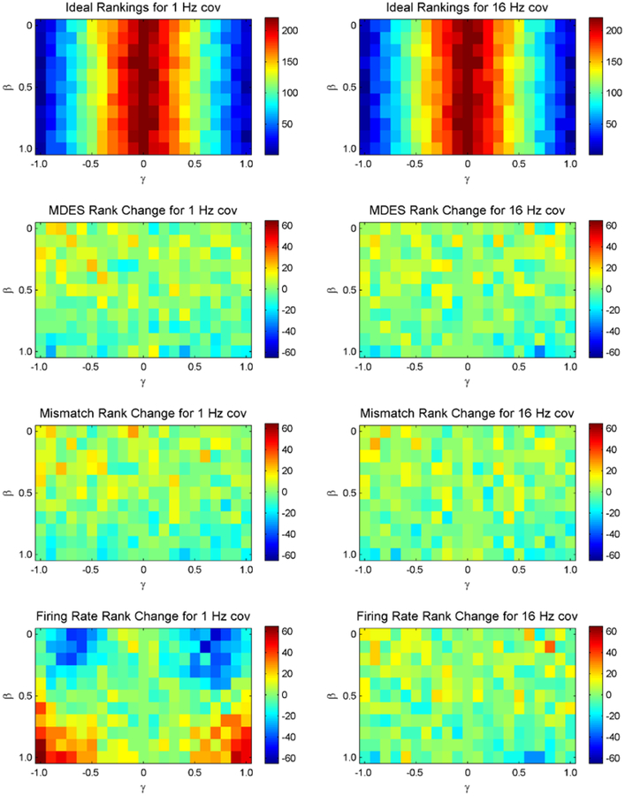
For 1 Hz and 16 Hz as the intrinsic covariate frequency, the 220 neurons with varying β and γ parameter values are ranked using MDES, firing rate, and the ideal standard based off of change time estimates. These rankings are shown in Figure 3 with the lower values (blue) denoting better rankings where each pixel denotes the ranking of a single neuron with a corresponding β and γ value. The ideal standard based on the most accurate change time estimates show that only the stimulus parameter, γ, matters when selecting neurons regardless of the frequency of the intrinsic covariate. The larger γ is, the better the neuron’s ranking with little to no variation based on the intrinsic covariate, β. The MDES rankings have a mean ranking difference of only 6.9 and 6.4 with the largest deviation as 33 and 22 for the 1 Hz and 16 Hz rankings respectively. There also is very little pattern in their deviations in both cases except for a slight favoring of the higher values of β. With the mismatched MDES rankings, the mean difference are 7.1 and 6.8 with the largest deviation as 28 and 29 ranks for the 1 Hz and 16 Hz rankings respectively. The mismatched MDES rankings also show a favoring of the higher values of β.
Figure 3.
Rankings across model parameters based on the change point detection ideal (row 1) along with differences between ideal rankings compared to MDES rankings (row2), mismatched MDES rankings (row 3) or firing rate rankings (row 4). The left column corresponds to rankings from intrinsic covariates of 1 Hz while the right column corresponds to rankings from 16 Hz. The lower values (blue) correspond to better rankings while the higher numbers (red) correspond to worse rankings. This means blue relates to the best rankings in the ideal standard. In the bottom three comparison graphs, green corresponds to similar rankings. The ranking for γ = 0 is not calculated and is just set to 221(worst ranking) in order to have a continuous axis.
However, the firing rate rankings are substantially different from the ideal standard. The rankings have a mean difference from the ideal of 16.6 and 7.7 with the largest deviation as 63 and 24 for the 1 Hz and 16 Hz rankings respectively. At the lower frequency for the intrinsic covariate, the best rankings as judged by firing rate base rankings are the ones with a large dependence on the stimulus (γ) with a small dependence on the intrinsic covariate parameter (β). There is a large bias of the rankings based off of the intrinsic covariate parameter (β). At the higher frequencies, the rankings match the MDES rankings in that they are primarily dependent on γ but have a slight favoring of higher values of β.
Overall, both the correct MDES rankings as well the mismatched MDES rankings match much more closely with the ideal rankings. They perform much better in the scenario of low frequency intrinsic dynamics and still performs slightly better in the case of higher frequency intrinsic dynamics. The correct MDES rankings also perform slightly better than the rankings from mismatched MDES. The crux of these improvements come from the fact that firing rate changes are not necessarily caused by the stimulus. For a single trial, it is likely for the slower intrinsic covariate oscillations to have a net effect (either inhibitory or excitatory) on the post-stimulus firing rate compared to the pre-stimulus firing rate. These intrinsics act as noise by artificially changing the firing rate from trial to trial thus increasing the variance of the firing rates across trials. For low frequency intrinsic dynamics, good firing rate rankings come from neurons whose stimulus parameter (γ) are comparatively larger than the non-stimulus parameter (β). Ideally, all neurons with a large stimulus parameter will rank equally well, but these intrinsic dynamics cloud the relationship between a neuron’s spiking activity and the stimulus for the firing rate rankings. Once they are accounted for, like in the MDES rankings, the true relationship is clear.
As noted before, both the MDES and firing rate rankings have a slight preference for larger values of β. This is likely a byproduct of how the data was simulated. Since the firing rate is exponentially tied to the covariates, a larger β leads to times with exponentially more spikes. It is easier to detect changes in spiking activity with more spikes as it essentially gives us more information. For example, the difference between 1 Hz and 2 Hz is very hard to distinguish when we only have 500 ms of activity while the difference between 10 and 20 Hz is much easier. Regardless, this small deviation from the ideal rankings would be a problem with all ranking methods as they are all limited by the amount of information available.
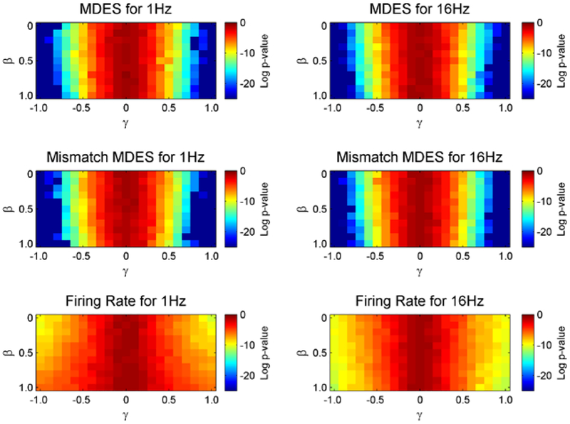
Next, p-values are examined between the MDES statistics and ANOVA test for firing rate (Figure 4). Only 5 new trials of spike trains are used to generate these figures to ensure the values are not too small to register. The p-values for the MDES method, both with the correct and mismatched model, are much smaller than for the firing rate method. This difference is most visible at the larger values of γ and can near an improvement of as much as 13 orders of magnitude. The difference lessens as γ shrinks.
Figure 4.
The Natural log of p-values is shown for both the MDES statistic and the ANOVA test for firing rate. The average is taken over 50 sets of neuron selection runs using only 5 trials. The columns show results for low and high frequency intrinsic covariates while the rows show results between the two selection methods. Values under −3 correspond to neurons that would have passed a 5% threshold for the p-value.
By using p-values < 5% as a threshold for selecting and rejecting neurons as task relevant, we can examine the sensitivity and specificity performance of both MDES and firing rate being used as a binary classifier. For the 1 Hz case, MDES has a sensitivity rate of 77.8% and 78.2% (mismatched) while firing rate only has a sensitivity rate of 69.2%. For the 16 Hz case, MDES’s sensitivity is 78.2% and 78.0% (mismatched) with firing rate having a sensitivity rate of 75.1%. To find the specificity, true negatives in this case are represented by neurons with γ = 0. Values are 95% are expected with the 5% threshold for the p-values. For the 1 Hz case, MDES has a specificity rate of 95.5% and 93.3% (mismatched) with firing rate having a specificity rate of 95.1%. For the 16 Hz case, MDES has a specificity rate of 95.6% and 95.8% (mismatched) with firing rate having a specificity rate of 94.9%. In general, these specificity rates are expected though MDES using a mismatched model has a larger number of false positives for the 1 Hz case.
With the correct model, MDES thus not only ranks neuron importance better than firing rate, it also is more powerful in finding neurons with task relevance. In the case of the mismatched model, MDES is able to still select for more task relevant neurons than firing rate ANOVA with the downside of lower specificity in the 1 Hz case (93.3% compared to 95.1%). The loss in specificity is tied to the strength of the model and its fit. More trials as well as cross validating model fits will mitigate the number of false positives.
3.2. Case 2 - Finger Movement Decoding
3.2.1. Experiment
This data was recorded by Dr. Marc Schieber at University of Rochester Medical Center. A male rhesus monkey (Macaca mulatta, NCBI Taxonomy: 9544) is trained to perform visually cued finger movements. Each movement consisted of either the extension or flexion of a digit or wrist. These are represented by an ‘e’ or ‘f’ relating to the extension or flexion followed by ‘1’-’5’ for the corresponding digit or ‘w’ for the wrist (e.g. ‘e4’ is the extension of the 4th digit). Neural recordings include 115 single units that cover the hand area of the primary motor cortex contralateral to the trained hand. These single units are already screened as being movement relevant based off their firing rate. Of these, any neurons with fewer than 10 trials in any of the movements are discarded. These recordings are not simultaneous but are assumed so for the purposes of the study. Trials under the same behavior but recorded separately can be grouped up and act as one simultaneous trial for either encoding or decoding. Details from the behavioral experiment can be found in [6].
3.2.2. Model
The full model includes, for each of the twelve movements, both a set of history covariates and a basal firing rate:
| (12a) |
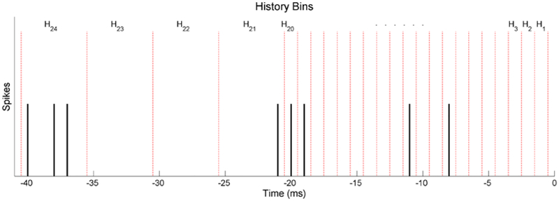
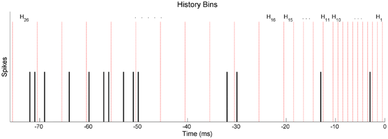
where m and h represent movement and history bin indices respectively. Im is an indicator function which is 1 only during its respective movement m, αm represents the basal frequency for the mth movement, Hh represents the number of spikes during the hth non-overlapping history window, and βm,h represents the respective parameter to be fitted. The most recent 20 history windows cover 1 ms each up until 20 ms in the past. The last four cover 5 ms each until a total of 40 ms in the past. The history bins are displayed in an example spike train in Figure 5. The fine resolution for the recent history windows is used to better resolve the refractory period. The null model follows the same form without different movement indices:
| (12b) |
Models are fit using all but three of the trials for every movement under every neuron which will be used for testing decoding performance. This leaves between 7 and 12 trials per movement per neuron in order to use for encoding. Again, these trial numbers might be different between movements under the same neuron since these trials were not simultaneously recorded.
Figure 5.
Example of a spike train with history bins used for M1 neuron models during dexterous finger movement models. The red dotted lines indicate the different bins. The history dependence covariates are the number of spikes contained in each of these bins, which are located 1–40 ms before the point in time being examined.
3.2.3. Method of Comparison
Decoding is used as a means of assessment for the success of the neuron selection and ranking. the decoding is performed using a maximum likelihood estimate across each of the possible movements of a new set of spike trains from a decoding pool of neurons that consists of the n ranked (either by MDES or firing rate or a completely random pool). For each movement to be decoded, one test trial from the three set aside is selected for each of the neurons. The likelihood of those spike trains given each of the twelve possible movements is calculated with the decoded movement having the largest likelihood:
| (13) |
where Ni represents the spike train from neuron i. This leads to one decoded movement. This process is repeated 100 times total for each movement with each repetition using a different random set of decoding trials. Furthermore, the entire process is repeated 10 times after a different set of trials is used for modeling and decoding.
3.2.4. Results
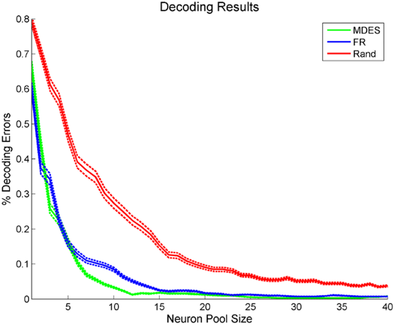
The resulting decoding accuracies are shown in Figure 6. Both the MDES and the firing rate selection methods greatly outperform random neuron selection. When comparing MDES and firing rate selection, MDES has the higher accuracy regardless most of neuron pool sizes. For pool sizes larger than 2, decoding with firing rate neurons is never significantly better than MDES neurons. This improvement is only 8% at most, however there is already limited room for improvement from the firing rate neuron’s decoding accuracy. Using MDES neurons, decoding approaches perfect decoding (8 neurons for 95%, 12 neurons for 99%) faster than the firing rate selection (12 neurons for 95%, 23 neurons for 99%). The results around 99% decoding accuracy show that on average 23 firing rate ANOVA selected neurons are needed to match the decoding power of only 12 MDES selected neurons.
Figure 6.
Accuracies for movement decoding as well as their 95% confidence interval using different rankings (MDES, firing rate, and a random pool) to select neuron pool. There are 95 neurons total to select from. Actively selecting neurons understandably greatly outperforms random selection. Decoding using MDES selected neurons performs the best regardless of neuron pool size though. A 95% decoding accuracy is reached within 8 neurons for the MDES selection while it takes 12 neurons using the firing rate ANOVA method.
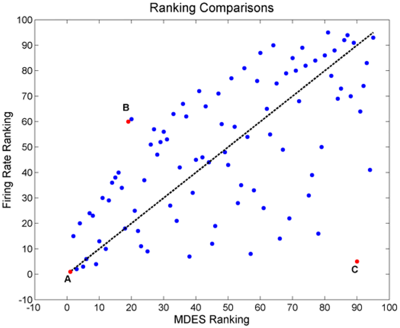
Figure 7 shows one relationship between the MDES ranking and the firing rate ranking as a means of comparing the two ordered sets. The first thing to note is that the two rankings are extremely different as seen from the deviation from y = x. Next, the best MDES ranked neurons tend to do well in terms of their firing rate ranking. However, there are numerous notable cases (e.g. point C highlight in Figure 7) where highly ranked neurons in terms of firing rate perform poorly in terms of the MDES ranking. Figure 7 is the result of only one iteration, but the relationships hold across each run and are thus robust to trial shuffling despite the exact rankings changing from run to run.
Figure 7.
Firing rate rankings with respect to their ranking from the MDES method. The dotted y = x represents perfect similarity between the two systems. There are numerous deviations between the two methods throughout the neurons. Most notably, the best firing rate ranked neurons can perform very poorly based off of MDES while the MDES neurons generally perform well according to firing rate. Neuron A is an example of a neuron that performs well in both methods while neuron B and C perform much better in one of the methods.
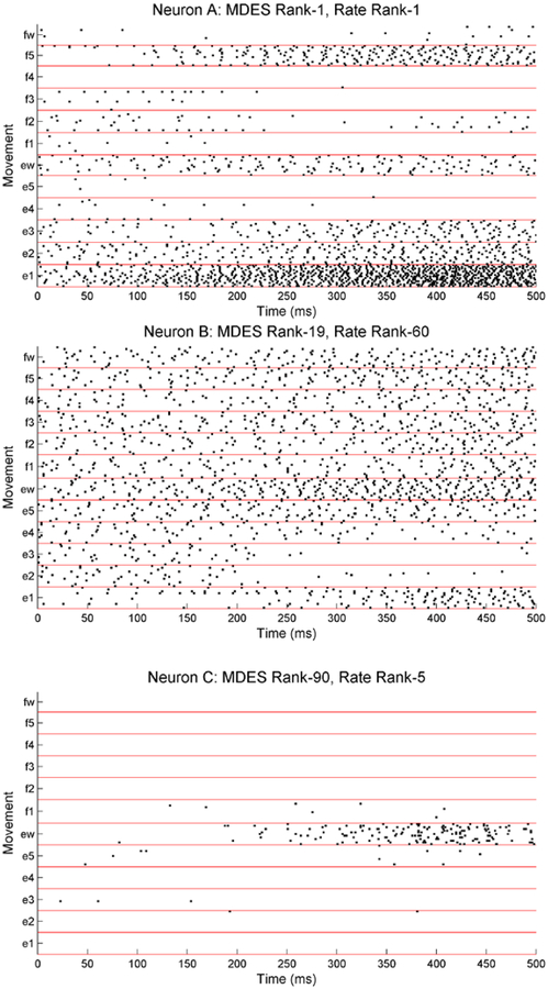
Taking a closer look at the raster plots (Figure 8) reveals how these rankings come about. Neuron A has very distinct firing rates across all movements and performs extremely well in both rankings. Neuron B with less significant changes in firing rates can still rank well with MDES when there are distinct differences in its history dependencies. Finally, neuron C behaves similarly for most of the movements despite having distinct activity in one movement. It ranks much worse with MDES since this method requires a large separation between the full and the null models. If 11 of the 12 movements have the same dynamics, then this separation will be a lot smaller. Though neuron C is able to easily distinguish the ‘ew’ movement, it gives us virtually zero information regarding the other 11 movements and would perform worse with decoding aside from that single movement. It is therefore not as task relevant as the other neurons and should not be considered amongst the best ranked neurons especially for decoding. However, it still has some task relevance and does pass the 5% significance level for both firing rate ANOVA and the MDES test statistic. All the neurons in fact easily pass since this data set has been prescreened for movement related neurons by examining firing rate.
Figure 8.
Raster plots with movement onset at 250 ms for three neurons as indicated by the highlighted neurons in Figure 6. Neuron A shows very distinct firing rate activity across most movements and thus ranks well both in MDES and in firing rate. Neuron B shows a much more homogenous firing rates across movements but has distinct history dependencies (not shown) and is able to rank well in MDES despite ranking poorly in firing rate. Lastly, neuron C only shows activity for the ‘ew’ movement. Since the other movements are virtually indistinguishable, the neuron ranks poorly in MDES despite ranking well in firing rate.
3.3. Case 3 - Action Value and Action Selection Related Neurons
3.3.1. Experiment
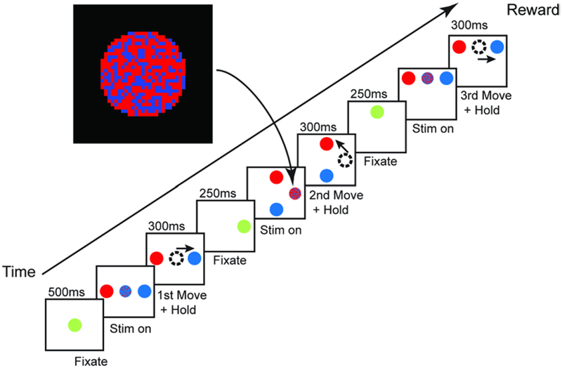
This experiment was performed by Dr. Bruno Averbeck at the National Institute of Mental Health. Two male adult Rhesus monkeys (Macaca mulatta, NCBI Taxonomy: 9544) were trained to perform a sequence of three visually cued saccades (Figure 9). The trial starts with the monkey fixating at a central green target. After fixation, the monkey is shown the stimulus, a circle with both red and blue pixels, as well as two possible targets, one of which is completely red and the other blue. The correct saccade target is signaled by the larger portion of colored pixels in the pixelated circle. After making the correct saccade, the correct circle turns green to signify another fixation period. A second saccade is signaled from this new location in the same manner as the first. The green fixation circle turning into the red and blue pixelated circle with a new blue and red target being shown as well. After another correct saccade, a third and final fixation and stimulus set is used to signal the last saccade. One trial consists of these three saccades in sequence. Additionally, the amount of color bias is changed from trial to trial. This dictates how heavily biased the stimulus’ color is towards the correct target color. During these trials, single unit recordings from both prefrontal cortex and striatum were obtained from the monkeys. Further details on experimental procedures can be found in [7].
Figure 9.
Monkey saccade task timeline. The monkey performs a sequence of three visually cued saccades. For each saccade, the monkey is shown a stimulus pixilated with two colors. The larger portion of the colors indicate the correct target to saccade to and hold. Only after the third saccade does the monkey receive a reward.
3.3.2. Modeling
Spike trains are organized from 200 ms before to 700 ms after stimulus presentation. The full model used is similar to the decoding example’s:
| (14a) |
where the indicator functions show when their respective parameters for which movement and color bias. The history windows used are the same as I the decoding case. The respective move-based and color-based null models are thus:
| (14b) |
and
| (14c) |
For the movement null model, the movement indicator is replaced with a fixation indicator. Fixation location is required in order to dissociate the activity related to the actual movement from the activity related to just the starting position.
3.3.3. Method of Comparison
The original study was successfully published with analysis from firing rate based neuron selection. The comparison in this case seeks to test if a parallel analysis with MDES based neuron selection will yield similar results. Neuron selection from firing rate is accomplished by an ANOVA test matching the one performed in the publication. Average firing rates are calculated using 100 ms moving windows (with 50 ms step sizes) from 200 ms before the stimulus to 700 ms after the stimulus. A three-way ANOVA test is used for each window with movement, color bias, and fixation. The p-values associated with movement and color bias are used to determine if a neuron is relevant to the respective task property (p<.05). In order to better compare the two methods, windowed spike trains are also used for MDES. The full and null models are fit using these 100 ms windows of data and neurons are selected based off of the p-values from MDES.
3.3.4. Results
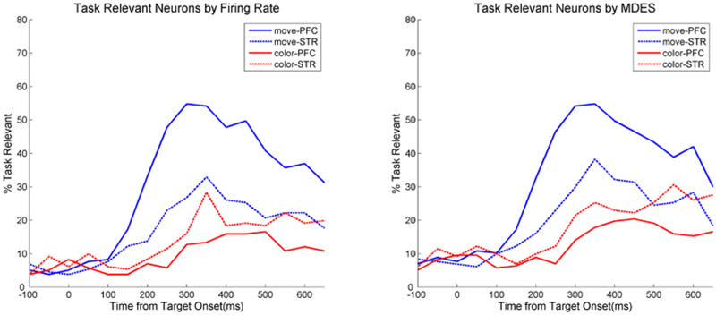
Firing rate and MDES neuron selection are both performed separately for prefrontal cortex and striatum neurons. The percentage of prefrontal and striatal neurons significant to either movement or color bias are shown over time in Figure 10. In both the firing rate and MDES selection, very few neurons are selected as relevant before the stimulus as expected. Once the stimulus is shown, the number of relevant neurons rises to reflect the amount of information about movement and color bias is represented in prefrontal versus striatal neurons. MDES selection gives very similar results in this case where firing rate was able to successfully capture the neuron’s behavior. It also obviously leads to the same neurophysiological conclusion that action selection (movement) is better represented in prefrontal cortex where action value (color bias) is better represented in striatum.
Figure 10.
Neurons relevant to movement or color bias in the task for either prefrontal or striatal neurons over time. There is very little qualitative difference between the selection using firing rate versus the selection using MDES. All traces start with very few relevant neurons before the stimulus and then grow to similar peak values after target onset before declining again.
3.4. Case 4 - Resolving Modulations in Oscillatory Activity
3.4.1. Experiment
This data was collected by Dr. Emad Eskandar at Mass General Hospital. Two healthy adult male Rhesus monkeys (Macaca mulatta, NCBI Taxonomy: 9544) were trained to perform a visually cued radial center-out motor task. Once centered (fixation ‘F’), eight gray objects appear in a radial arrangement equidistant from the center of the screen (stimulus ‘S’). One of the eight gray targets is randomly chosen and replaced by a green circle (onset of cue ‘C’), which instructs the animal to move (onset of movement ‘M’) its hand towards that target and hold the position. Extracellular microelectrode recordings are made from the internal Globus Pallidus (GPi) during the behavioral task. Electrodes are introduced into the brain through a 1mm spaced grid and are advanced until the activity of one or more neurons is well isolated. No task related neuron selection is performed at this point. Further details on experimental procedures can be found in [8].
3.4.2. Modeling
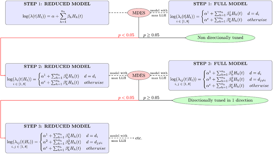
The neuron spike trains are modeled in a 400 ms time window centered at 150 ms before the onset of movement. We perform a stepwise likelihood ratio test to determine the directionally tuned neurons (Table 1).
Table 1:
Flowchart showing the stepwise MDES method. LLH = likelihood.
|
MDES was used in a stepwise manner in order to recover all the directions that may be tuned in each neuron. At each row in the flow chart, an MDES test is performed between the null and full models to test. The first step tests if at least one of the 8 directions significantly modulates activity compared to the rest. Note that in the full model’s first step of the flowchart, the likelihood is maximized over 8 possible di’s. If at least one direction is significant, the second step tests if 2 directions significantly modulate. The likelihood is thus maximized over the 27 possible pairs of directions {di, dj≠i}. The number of directions tested at once increases with each step until there is no significance found. At that point, the most significant models of the previous step is selected to indicate directional tuning.
Although we only maximize the likelihood of the model over a discrete set of directions, it is conservative to add an extra degree of freedom for each direction that has a separate set of parameters. For example, in the full model’s first step, the model with the maximum likelihood has (nh + 2) degrees of freedom. The stepwise MDES method is performed for each neuron as in the flowchart till the MDES test in one of the steps is not passed at the desired significance level. In this case, the null model at that step is chosen as a model for that neuron; if any of the directions have a separate set of parameters to describe their activity in this model, the neuron is tuned in these directions. The history windows (Figure 11) are chosen based on related studies on directional tuning [30].
Figure 11.
Example of a spike train with history bins used for GPi neuron models during center out movement models. The red dotted lines indicate the different bins. The history dependence covariates are the number of spikes contained in each of these bins, which are located 1–75ms before the point in time being examined.
We acknowledge that stepwise MDES is a computationally intensive method to retrieve tuned neurons. In case of lack of adequate computational resources, from the second step onwards, the stimuli that have been shown to be tuned in the previous steps can be fixed. This will decrease the number of models needed to be generated in each subsequent step though the likelihood might not be a true global maximum.
3.4.3. Method of Comparison
As a comparison, we identify neurons that display a significant change in firing rate in a 400 ms window centered at 150 ms before movement. Each neuron is tested for directional tuning by using the ANOVA test. If the neuron passes the ANOVA test (p<0.05), then the neuron’s activity modulates with respect to at least some directions. In order to find which directions the neuron is tuned for, a multiple comparisons pairwise test is performed. A direction is tuned if it’s firing rate for that direction is significantly different from the firing rate of at least half of the other directions. Note that a neuron may be tuned in more than one direction.
Next, the oscillatory characteristics of the neurons in the beta (9–25 Hz) and gamma (40–90 Hz) frequency bands were assessed using the power spectrum density (PSD) with the Welch method [31] given directionally tuned neurons that were identified using the two different methods (MDES and firing rate ANOVA). We considered one window (400 ms long) around each marker: ‘F’, ‘S’, ‘C’ and ‘M’. In addition, we considered 1 additional overlapping window after ‘C’, and 5 overlapping windows before ‘M’ (400 ms long, overlapping by 50 ms). For each window, the average normalized power in the beta band (Pβ) and gamma band (Pγ) was estimated as in [32] (normalized power is referred to as SNR in [32]). Normalized power values that fell below 0 were not considered in this analysis. If the neuron was directionally tuned, only trains recorded during tasks involving the tuned direction were considered. For non-directionally tuned neurons, all spike trains were considered.
3.4.4. Results
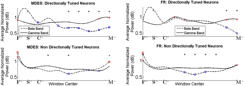
A total of 83 neurons were isolated from the GPi from two non-human primates (monkey 1, n = 27; monkey 2, n = 56). We identified 46 and 25 neurons that were tuned using MDES and firing rate ANOVA respectively. We show the Pβ and Pγ values for directionally tuned and non-directionally tuned neurons for the duration of the entire trial in Figure 12 Left, with the directionally tuned neurons identified using MDES. We see that Pβ is above Pγ until the cue is observed. After the presence of the cue, we see that Pβ decreases significantly with respect to baseline, while Pγ is significantly higher than baseline in the two windows preceding movement. Moreover, Pγ is significantly higher than Pβ for most of the time between cue and movement onset. This ‘cross-over’ effect, i.e., the emergence of high power in the gamma band concurrently with a decrease in beta power is only seen in the directionally tuned neurons. In the non-directionally tuned neurons, no consistent trend is noticed in the beta and gamma band power.
Figure 12.
Population-averaged normalized power in the beta (Pβ, 9–25 Hz, dashed lines) and gamma (Pγ, 40–90 Hz, solid lines) frequency band on overlapping windows for directionally tuned neurons (top row) and non-tuned neurons (bottom row), as identified by two different methods. Left: Tuned neurons identified using the MDES method; Right: Tuned neurons identified using a difference in firing rates. Blue squares / circles indicate a decrease, while red squares / circles indicate an increase (one sided t-test, p<0.05) in Pβ / Pγ respectively, as compared to baseline, which is taken as 400 ms around ‘S’. The plus / cross signs indicate that Pγ / Pβ in that window is significantly higher than Pβ / Pγ in the same window, respectively. F = fixation; S = onset of grey circles; C = onset of cue; M = movement onset. The minus sign indicates that the window contains data from before the respective marker. Details on windows are provided in the methods.
In Figure 12 Right, we show a similarly computed graph with the tuned neurons identified using a change in FR, as detailed above. Though similar trends are seen as in Figure 12 Left, these trends are less pronounced and start later. Note that a slight cross-over effect is present in the directionally tuned neurons only just before the onset of movement. The MDES method, however, succeeds in recovering directionally tuned neurons that show a pronounced cross-over effect, which is hypothesized as being one of the key factors in the planning of movement [29,30]. Using the firing rate selected neurons in analysis would lead to the incorrect conclusion that a decrease in Pβ as well as a significant difference between Pβ and Pγ only occurs immediately prior to movement as opposed to during the entire planning stage.
As noted above, this stepwise MDES can become computationally intensive. Using a 2.5 GHz processor, the mean runtime for one neuron was 12.72 minutes while the median was 3.21 minutes. Each consecutive step becomes more costly with the additional number of covariates to model as well as the additional permutations of directions to maximize over. The average runtime for the fifth step (furthest any neuron ever got) is 21.5 minutes while the first step only averaged 0.46 minutes. Time can be saved in this scenario by assuming that the tuned direction found in step 1 is now fixed as tuned in step 2 and that both the tuned directions in step 2 are fixed in step 3. This leaves only 7 models to be built in step 2 instead of 28 (8 choose 2) and 6 models to be built in step 3 instead of 56 (8 choose 3). In general however, these computational costs depend a lot on the situation as they scale with the types of models used, the number of covariates, the number of possible tunings, as well as the degree of tuning in the neuron population.
4. Conclusions
4.1. Further Uses
Although we focus on a very particular realization of MDES in this study, this method can be easily generalized. All the models here are constructed using a generalized linear model framework for a point process model, but one can use any model for which a likelihood can be calculated. Also, most of the models we focus on take into account history dynamics as the intrinsic task irrelevant parameters. This does not have to be the case. With the increasing number of neurons that can be simultaneously recorded from, network dynamics should become an extremely useful model parameter. MDES can test for functional relationships by seeing if a neuron’s response to a stimulus can be explained more by the stimulus or by the input of neighboring neurons. Note that this does not imply causality as MDES cannot account for the confound of an unrecorded source and can only test functional relationships.
Additionally, MDES is not even limited to spike train observations. Local field potentials from electroencephalograms (EEGs) and electrocorticograms (EcoGs) can be use with MDES to select for relevant channels as well. Furthermore, this test can be expanded for multiple relevant task parameters. It is possible to have two independent task parameters (e.g. image type and image position for a visual task) and use this test to tease apart which neurons are related to which parameter or both or none.
4.2. Modeling Power
In the end however, the power of this test relies on the power of the model. If the model is not able to fully capture the dynamics of the data, then this and all model based rankings are less useful. As shown in the simulation, a mismatched model can result an increase in false positives. More data can improve model fits and cross validating can assess which models to trust. However, if there is not enough data to construct good models though, no neuron selection method will work well. With accurate models, we have been able to show the importance of taking into account the role history dependence and task irrelevant parameters. The MDES test is able to keep these factors in mind while making the rankings and selections of task relevance. Solely using firing rate makes the selection process particularly susceptible to noise generated by these parameters which are task irrelevant, but still spiking dependent. The MDES test is able to accurately rank the neurons based off of how much information they hold regarding a task or stimulus. Following these rankings, higher decoding accuracies can be achieved with fewer neurons and neurophysiological effects dependent on task relevance can be more cleanly resolved.
Acknowledgements
K Kahn and SV Sarma were supported by the Burroughs Wellcome Fund CASI Award (100727401) and the National Science Foundation - Emerging Frontiers in Research and Innovation Award (1137237).
References
- 1.Brown EN, Kass RE, Mitra PP (2004) Multiple neural spike train data analysis: state-of-the-art and future challenges. Nature Neuroscience 7(5):456–61. [DOI] [PubMed] [Google Scholar]
- 2.Wahnoun R, He J, Helms Tillery SI (2006) Selection and parameterization of cortical neurons for neuroprosthetic control. Journal of Neural Engineering 3(2):162–71. [DOI] [PubMed] [Google Scholar]
- 3.Jensen W, Rousche PJ (2006) On variability and use of rat primary motor cortex responses in behavioral task discrimination. Journal of Neural Engineering 3(1):L7–13. [DOI] [PubMed] [Google Scholar]
- 4.Amirikian B, Georgopoulos AP (2000) Directional tuning profiles of motor cortical cells. Neuroscience Research 36(1):73–9. [DOI] [PubMed] [Google Scholar]
- 5.Singhal G, Aggarwal V, Acharya S, Aguayo J, He J, Thakor N (2010) Ensemble fractional sensitivity: a quantitative approach to neuron selection for decoding motor tasks. Computational Intelligence and Neuroscience 648202. [DOI] [PMC free article] [PubMed] [Google Scholar]
- 6.Schieber MH (1991) Individuated finger movements of rhesus monkeys: a means of quantifying the independence of digits. J. Neurophys 65(6): 1381–91. [DOI] [PubMed] [Google Scholar]
- 7.Seo M, Lee E, Averbeck BB. (2012) Action Selection and Value in Frontal-Striatal Circuits. Neuron, 74: 947–960. [DOI] [PMC free article] [PubMed] [Google Scholar]
- 8.Saxena S, Gale JT, Eskandar EN, Sarma SV (2011) Modulations in the oscillatory activity of the globus pallidus internus neurons during a behavioral task-a point process analysis Conf Proc IEEE Eng Med Biol Soc, 4179–4182 [DOI] [PMC free article] [PubMed] [Google Scholar]
- 9.Brown EN, Frank LM, Tang D, Quirk MC, Wilson MA (1998) A statistical paradigm for neural spike train decoding applied to position prediction from ensemble firing patterns of rat hippocampal place cells. Journal of Neuroscience 18:7411–25. [DOI] [PMC free article] [PubMed] [Google Scholar]
- 10.Eden UT, Frank LM, Barbieri R, Solo V, Brown EN (2004) Dynamic analyses of neural encoding by point process adaptive filtering. Neural Computation 16(5):971–998. [DOI] [PubMed] [Google Scholar]
- 11.Saleh M, Takahashi K, Amit Y, Hatsopoulos NG (2010) Encoding of coordinated grasp trajectories in primary motor cortex. Journal of Neuroscience 30(50):17079–90. [DOI] [PMC free article] [PubMed] [Google Scholar]
- 12.Santaniello S, Gale JT, Montgomery EB, Sarma SV (2010) Modeling the effects of Deep Brain Stimulation on sensorimotor cortex in normal and MPTP conditions Conf. Proc. IEEE Eng. Med. Biol. Soc. 2081–4. [DOI] [PMC free article] [PubMed] [Google Scholar]
- 13.Santaniello S, Gale JT, Montgomery EB, Sarma SV (2010) Modeling the motor striatum under Deep Brain Stimulation in normal and MPTP conditions Conf. Proc. IEEE Eng. Med. Biol. Soc. 2065–8. [DOI] [PMC free article] [PubMed] [Google Scholar]
- 14.Santaniello S, Gale JT, Montgomery EB, Sarma SV (2012) Reinforcement mechanisms in putamen during high frequency STN DBS: A point process study Conf. Proc. IEEE Eng. Med. Biol. Soc. 1214–7. [DOI] [PMC free article] [PubMed] [Google Scholar]
- 15.Santaniello S, Montgomery EB, Gale JT, Sarma SV (2012) Non-stationary discharge patterns in motor cortex under subthalamic nucleus deep brain stimulation. Front. Integr. Neurosci 6(35). [DOI] [PMC free article] [PubMed] [Google Scholar]
- 16.Sarma SV, Cheng M, Eden U, Hu R, Williams Z, Brown EN, et al. (2008) Modeling neural spiking activity in the sub-thalamic nucleus of Parkinson’s patients and a healthy primate 47th IEEE Conf. Decis. Control 2012–7. [DOI] [PMC free article] [PubMed] [Google Scholar]
- 17.Sarma SV, Cheng ML, Eden U, Williams Z, Brown EN, Eskandar EN (2012) The effects of cues on neurons in the basal ganglia in Parkinson’s disease. Front. Integr. Neurosci 6(40). [DOI] [PMC free article] [PubMed] [Google Scholar]
- 18.Saxena S, Santaniello S, Montgomery EB, Gale JT, Sarma SV (2010) Point process models show temporal dependencies of basal ganglia nuclei under deep brain stimulation Conf. Proc. IEEE Eng. Med. Biol. Soc. 4152–5. [DOI] [PMC free article] [PubMed] [Google Scholar]
- 19.Saxena S, Gale JT, Eskandar EN, Sarma SV (2011) Modulations in the oscillatory activity of the Globus Pallidus internus neurons during a behavioral task-A point process analysis Conf. Proc. IEEE Eng. Med. Biol. Soc. 4179–82. [DOI] [PMC free article] [PubMed] [Google Scholar]
- 20.Saxena S, Schieber MH, Thakor NV, Sarma SV (2012) Aggregate input-output models of neuronal populations. IEEE Trans. Biomed. Eng 59(7):2030–9. [DOI] [PMC free article] [PubMed] [Google Scholar]
- 21.Brown EN, Barbieri R, Eden UT, Frank LM (2003) Likelihood methods for neural spike train data analysis In: Feng J, ed. Computational neuroscience: a comprehensive approach London: CRC, Chapter 9, 253–286. [Google Scholar]
- 22.Kahn K, Sheiber M, Thakor N, Sarma SV (2011) Neuron selection for decoding dexterous finger movements Conf. Proc. IEEE Eng. Med. Biol. Soc. 4605–8. [DOI] [PubMed] [Google Scholar]
- 23.Coleman TP, Sarma SS (2010) A computationally efficient method for nonparametric modeling of neural spiking activity with point processes. Neural Comput 22(8):2002–30. [DOI] [PubMed] [Google Scholar]
- 24.Sarma SV, Nguyen DP, Czanner G, Wirth S, Wilson MA, Suzuki W, et al. (2011) Computing confidence intervals for point process models. Neural computation 23(11):2731–45. [DOI] [PubMed] [Google Scholar]
- 25.Snyder D, Miller M (1991) Random point processes in time and space New York: Springer-Verlag. [Google Scholar]
- 26.Cox DR, Isham V (1980) Point Processes London: Chapman & Hall. [Google Scholar]
- 27.Brown EN (2005) Theory of Point Processes for Neural Systems In: Chow CC, Gutkin B, Hansel D, Meunier C, Dalibard J, eds. Methods and Models in Neurophysics Paris, Elsevier; Chapter 14, 691–726. [Google Scholar]
- 28.Truccolo W, Eden UT, Fellow MR, Donoghue JP, Brown EN (2005) A point process framework for relating neural spiking activity to spiking history, neural ensemble and extrinsic covariate effects. J. Neurophys 93: 1075–89 [DOI] [PubMed] [Google Scholar]
- 29.McCullagh P, Nelder A (1989) Generalized Linear Models, 2nd ed., London: Chapman & Hall. [Google Scholar]
- 30.Saxena S (2011) Neuronal Activity of the Globus Pallidus Internus: Correlates Related to Cued Movements, Parkinson’s Disease, and Deep Brain Stimulation Diss. Johns Hopkins University. [Google Scholar]
- 31.Welch PD (1967) The Use of Fast Fourier Transform for the Estimation of Power Spectra: A Method Based on Time Averaging over Short, Modified Periodograms. IEEE Trans. Audio Electroacoustics, AU-15: 70–73. [Google Scholar]
- 32.Gale JT, Shields DC, Jain FA, Amirnovin R, Eskandar EN (2009) Subthalamic Nucleus Discharge Patterns During Movement in the Normal Monkey and Parkinsonian Patient. Brain Res 1260: 15–23. [DOI] [PMC free article] [PubMed] [Google Scholar]


