Abstract
Purpose
Robust and reliable reconstruction of images from noisy and incomplete projection data holds significant potential for proliferation of cost‐effective medical imaging technologies. Since conventional reconstruction techniques can generate severe artifacts in the recovered images, a notable line of research constitutes development of appropriate algorithms to compensate for missing data and to reduce noise. In the present work, we investigate the effectiveness of state‐of‐the‐art methodologies developed for image inpainting and noise reduction to preserve the quality of reconstructed images from undersampled PET data. We aimed to assess and ascertain whether missing data recovery is best performed in the projection space prior to reconstruction or adjoined with the reconstruction step in image space.
Methods
Different strategies for data recovery were investigated using realistic patient derived phantoms (brain and abdomen) in PET scanners with partial geometry (small and large gap structures). Specifically, gap filling strategies in projection space were compared with reconstruction based compensation in image space. The methods used for filling the gap structure in sinogram PET data include partial differential equation based techniques (PDE), total variation (TV) regularization, discrete cosine transform(DCT)‐based penalized regression, and dictionary learning based inpainting (DLI). For compensation in image space, compressed sensing based image reconstruction methods were applied. These include the preconditioned alternating projection (PAPA) algorithm with first and higher order total variation (HOTV) regularization as well as dictionary learning based compressed sensing (DLCS). We additionally investigated the performance of the methods for recovery of missing data in the presence of simulated lesion. The impact of different noise levels in the undersampled sinograms on performance of the approaches were also evaluated.
Results
In our first study (brain imaging), DLI was shown to outperform other methods for small gap structure in terms of root mean square error (RMSE) and structural similarity (SSIM), though having relatively high computational cost. For large gap structure, HOTV‐PAPA produces better results. In the second study (abdomen imaging), again the best performance belonged to DLI for small gap, and HOTV‐PAPA for large gap. In our experiments for lesion simulation on patient brain phantom data, the best performance in term of contrast recovery coefficient (CRC) for small gap simulation belonged to DLI, while in the case of large gap simulation, HOTV‐PAPA outperformed others. Our evaluation of the impact of noise on performance of approaches indicated that in case of low and medium noise levels, DLI still produces favorable results among inpainting approaches. However, for high noise levels, the performance of PDE4 (variant of PDE) and DLI are very competitive.
Conclusions
Our results showed that estimation of missing data in projection space as a preprocessing step before reconstruction can improve the quality of recovered images especially for small gap structures. However, when large portions of data are missing, compressed sensing techniques adjoined with the reconstruction step in image space were the best strategy.
Keywords: compressed sensing, image inpainting, partial geometry, positron emission tomography
1. Introduction
Positron emission tomography (PET) is a noninvasive functional imaging technique that allows visualization and quantification of metabolic and physiological processes in the body.1 It enables various clinical and preclinical applications such as cancer diagnosis, disease staging, therapeutic evaluation, and drug discovery.2 The quality and quantitative accuracy of the images reconstructed from tomographic data strongly depend on the detector coverage by the system, which is a major cost factor. Most current scanners consist of tightly packed detector blocks to achieve satisfactory images. However, cost has been an important hindrance to proliferation of PET, especially in the developing world, and has limited their utility in clinics or research centers. Indeed, decreasing detector coverage can significantly reduce the cost of scanners. To preserve the quality of recovered images, appropriate compensation techniques are required to reduce distortions caused by limited number of PET detectors. In the early 2000s, some comparisons were made between full ring and partial ring PET scanners.3 Nonetheless, this was prior to the emergence of advanced image recovery methods such as inpainting and compressed sensing, which have shown significant potential and are the focus of this study.
In the present study, two different strategies for data recovery in a PET scanner with partial geometry are implemented and compared; namely, gap filling strategies in projection space (so‐called sinogram inpainting) and compensation strategies in image space using compressed sensing (CS) based image reconstruction. Our aim was to assess whether missing data recovery is best performed in the projection domain prior to image reconstruction or within the reconstruction step in image space. We chose to do these individually to better understand the underlying differences in these two approaches.
Image inpainting is the process of filling in missing parts of damaged images based on information gathered from surrounding areas.4 Image inpainting has been widely investigated in different image restoration applications; e.g., scratch or text removal in photographs,5 digital effects (e.g., removal or replacement of unwanted objects6), image coding and transmission (e.g., recovery of the missing blocks7), artifact reduction (e.g., metal artifact removal from medical imaging8, 9), etc.
CS is a valuable method capable to accurately reconstruct a signal from fewer samples than is assumed to be required based on the Nyquist theorem.10 CS‐based signal recovery is possible when signal is sparse in some domain, which is commonly observed in medical images. This technique has been widely used for magnetic resonance imaging (MRI) and computed tomography (CT) image reconstruction,11, 12 where decreasing the scan time and radiation exposure of patients have always been important concerns with these techniques. However, employing CS recovery techniques in PET imaging are less explored.13, 14
In this work, we have investigated the effectiveness of the state‐of‐the‐art methodologies for sinogram inpainting and CS to preserve the quality of reconstructed images from two clinical undersampled PET data.
2. Materials and methods
2.A. Sinogram inpainting
Image inpainting, also known as image completion or disocclusion, is a technique used to recover the image regions, which are missing or damaged, in a visually plausible manner to make the corrupted image more discernible. There are numbers of method used for image inpainting.15 Here, we review some techniques that have been relatively successful in filling the gap structure in sinogram format PET data with partial geometry.
2.A.1. Partial differential equation techniques
Partial differential equation (PDE)‐based image inpainting techniques have attracted much research attention in the field of digital image processing since the 1990s.16 The mathematical models borrow ideas from classical fluid dynamics and heat conduction to tackle image inpainting. Using these methods, the image can be treated as heat, fluid, or gas that diffuses from the area of high concentration to the area of lower concentration. The heat equation is commonly used as the inpainting model,16 where the gray‐scale value of each pixel is considered as some physical quantity, and the image inpainting process is performed by modeling the physics of the phenomenon. By iteratively solving the numerical representation of a PDE, via variational methods,17 the information of gray values from surrounding areas are smoothly propagated into the corrupted region along equipotential lines (lines of equal light intensity).
Let be the given partial sinogram with inpainting domain , then the inpainted sinogram u can be recovered by minimizing of a suitable energy function.17, 18 Various nonlinear PDEs have been developed to capture important geometric features of the image for inpainting. To preserve edges as one of the most important features in images, total variation‐based PDE was proposed as Eq. (1). Since the model is the second‐order variational approach, we refer to it hereafter as PDE2.
| (1) |
The main drawback of PDE2 is that the equipotential lines are interpolated linearly. Therefore, the curvatures of lines are not preserved, which may result in straight line connections across the missing domain that may produce unsatisfactory outcome in the presence of large gap.
To overcome this problem, a solution might be obtained through the use of higher order PDEs. A recently developed fourth order inpainting algorithm for binary images based on PDEs is the Cahn–Hilliard approach.19 This approach is based on a physical model of fluid phase separation, and is given by:
| (2) |
where is a so‐called double‐well potential, e.g., , and λ is the same as defined before by Eq. (1) and parameter ϵ determines the steepness of the transition between 0 and 1. The Cahn‐Hilliard approach (which we refer to hereafter as PDE4) has the desirable property of curvature based inpainting models in term smooth continuation of level lines into the missing domain.
A generalization of the Cahn–Hilliard inpainting approach to gray value images has been proposed in Ref. 18. In the inpainting task, planning the efficient numerical schemes to acquire the right solution of proposed models is still a challenge. The efficient numerical solution of several inpainting equations presented in Ref. 20 use a semi‐implicit scheme that are guaranteed to be unconditionally stable. In this study, we used the numerical schemes proposed in Ref. 20.
2.A.2. Total variation regularization
The total variation concept was introduced by Rudin et al.21 for image denoising, and numerous applications including image zooming, inpainting, deblurring, compressive sensing, etc. Total variation regularization is based on the principle that noise or gap distortion in images will manifest as small variations throughout the image. As a result, the integral of the absolute gradient of the image may be high due to large number of small variation. This is defined for a differential function u, by
| (3) |
Interestingly, when used in image processing this functional removes elements with small gradients, typically associated with noise or gap distortion, while preserving important details such as edges.
Given a model for image acquisition, where a device captures P noisy measurements f of the high‐resolution image :
| (4) |
where ε is an additive noise and operator Φ accounts for missing data. Total variation can be used as a regularization term to inpaint an image as follows:
| (5) |
where γ is related to the noise standard deviation, and can be estimated known a priori.
However, if noise is unknown, the problem is often better reformulated as follow:
| (6) |
Several algorithms have been proposed to solve this problem,22, 23, 24 and projected gradient descent has been shown to be very effective.25 In this study, we applied the projected gradient descent method proposed by Ref. 25 to our experimental results.
2.A.3. DCT‐based penalized regression
The discrete cosine transform (DCT) can be used as an inpainting method via penalized least squares to fill the missing data in sinograms and as well to suppress the artifact.26 The method, originally proposed for automatic smoothing of incomplete data,27 it is used in this study for the same purpose.
This method solves the problem given by,
| (7) |
where f represents the partial observation in sinogram space, W a weight matrix of the same size allocating high value to high quality data and low value to missing data, Δ and stand for the Laplace operator and element‐wise product, respectively, while γ is a regularization term that controls the degree of smoothness, and u is a gap filled sinogram. As shown in Ref. 27, can be found by rewriting Eq. (7) with type‐II DCT and its inverse.
2.A.4. Dictionary learning based inpainting
Sparse dictionary learning is a popular representation learning approach, which aims to find a sparse representation of the input data in the form of a linear combination of basic elements (so‐called atoms), while simultaneously learning those basic elements themselves to form a dictionary. This is important because the performance of sparse representation methods is dependent on representing the signal as sparsely as possible. Some kinds of signals may be sparsely represented under some predefined dictionaries based on Fourier, wavelet, curvelet, and other transforms. However, a dictionary that is trained to fit a particular type of input data can significantly improve the sparsity and show improved performance. Indeed, training an adaptive dictionary based on image patches is able to preserve local structures and details for image recovery.
In this work, the following problem (which we refer to hereafter as DLI) is solved. Suppose u has a sparse representation under a dictionary D; then given linear measurement , the basic objective function is defined as follows:
| (8) |
where counts the nonzero number of its entity and L represents sparsity constrain.
Several techniques have been proposed to solve the problem defined by Eq. (8), and can be divided into two broad classes:
-
(a)
The first group is based on optimization techniques that iterate between a representative set of sparse coefficient (estimated typically via Orthogonal Matching Pursuit,28 Basis Pursuit,29 Iterative Hard Thresholding,30 and etc.31) and update of the dictionary using known sparse coefficients (utilizing algorithms such as K‐Singular Value Decomposition,32 gradient descent,33 and etc.). In these techniques, the stopping criterion is defined by assuming knowledge of the noise variance or sparsity level of sparse coefficients α.
-
(b)
The second group of techniques for sparse representation and dictionary learning is based on the Bayesian concept which considers a statistical model of data while all parameters of the model are directly inferred from data.
Generally, optimization techniques have the advantage of faster convergence in comparison to Bayesian one, but require several parameters that need to be tuned. In this study, we used nonparametric Bayesian dictionary learning for sparse representation of our simulated PET sinograms.34
2.B. Compressed sensing based image reconstruction
CS is a powerful framework to reliably recover a signal from fewer samples than is basically assumed to be required based on Nyquist theorem.10 CS‐based signal recovery is possible when the signal is sparse in some domain. In fact, given the correct sparse domain it is possible to perfectly reconstruct a noisy signal. Medical images often meet this criterion, and the Shepp–Logan phantom which usually serves as the model of a human head has sparsity in the gradient magnitude domain of the image as shown in Fig. 1. This means that, while the intensities of most pixels in the original image domain are not zero, the gradient magnitude transform domain significantly increases the number of zero pixels that correspond to the underlying signal.
Figure 1.
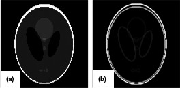
(a) Shepp–Logan phantom; (b) magnitude of the image gradient.
In this regard, a PET reconstruction algorithm can be formulated with a constraint on partially sampled data as follows:
| (9) |
where f is the partial observation in sinogram space , y is the reconstructed image, Ψ is the transform operator to a sparsifying domain, A is the PET scanner system matrix, and γ is the regularization parameter, and notation <.,.> refers to inner product of two vectors ().
In what follows, we outline sparse domains of significant potential for reconstruction of PET data with partial measurements.
2.B.1. Total variation
The gradient magnitude domain is one of the most commonly used sparsifying domains for medical images. Accordingly, to recover the sparsity of an image during reconstruction, TV minimization of the estimated image might be a solution. CS recovery of PET data using TV minimization can be formulated as follow:
| (10) |
where is isotropic or anisotropic total variation as defined in Ref. 35.
Since the objective function in Eq. (10) is nondifferentiable due to TV regularization term, traditional gradient‐type and expectation maximization‐type algorithms fail to find the optimal solution. To address this problem, recent techniques like PAPA,36 ADMM,37 or Chambolle–Pock38 have been proposed. In this study, we applied the PAPA technique to optimize the TV regularization model as defined by Eq. (10), and refer to it as TV‐PAPA.
2.B.2. Higher order total variation
TV‐based reconstruction in the presence of noise often results in blocky appearances (piecewise constant regions, i.e., “staircase” artifacts) in the image.35 Consequently, the finer details of the image may not be appropriately recovered. Additionally, the regions of the image that contain weak gradients may appear as piecewise constant in the reconstructed image. To address these problems, CS based on higher order discontinuity penalties has been proposed.35 This can be achieved by introducing higher order derivatives into Eq. (10). Here, we used the PAPA technique, solving higher order TV regularization as described in Ref. 35, and refer to it as HOTV‐PAPA.
2.B.3. Dictionary learning based CS
Unlike Section 2.A.4, which trains a dictionary over the PET sinogram to recover the missing pixels, here we directly apply dictionary learning and sparse representation to the reconstructed image, and formulate the optimization problem as follow:
| (11) |
where f is the partial sinogram, y is the reconstructed image, D and x represent the dictionary and its corresponding coefficients, respectively.
In order to solve Eq. (11), the problem is again split into two steps:
| (12) |
| (13) |
Equation (12) is the same as Eq. (8) which has been already discussed for determining D and x. Given D and x, then y is simply estimated as , and for an initial estimate of y, the objective function defined by Eq. (13) can be easily optimized by standard PET reconstruction algorithms like MLEM or OSEM.39, 40, 41
3. Results
3.A. Metrics and studies
This study compares the performance of the various methods using simulated data, which implies some type of estimation task. Both root‐mean‐square error (RMSE), and structural similarity index (SSIM) are good generic candidates for this purpose. To evaluate the quality of reconstructed images, we used RMSE, restricted to the reference images support, and SSIM of the images.42, 43
Three studies were performed to assess the performance of the algorithms; experiments on two realistic clinical images. Because we used real patient PET images to recreate the undersampled projection data, we refer to both data sets as patient derived phantoms (patient brain phantom and patient abdomen phantom). To realistically simulate data from real patient images for both studies (we did not directly work with real patient sinograms), we simulated attenuation, scatter and random data to create realistic sinograms, as described in PETSTEP.44, 45 Using these images for our simulation has distinct advantage of not being piecewise constant. This is important in this study because piecewise constant phantoms would mask the complexity of the missing data, which could lead to difficulty in properly evaluating the various inpainting methods. For all studies, Poisson noise is added to the sinogram to make the experiments consistent with real data. All experiments were run with 20 noise realizations for each noise level, and the results reported are the mean values. The figures depicted here are based on one noise realization; however, the mean and variance images are shown in Data S1 (Figs. [Link], [Link], [Link], [Link]).
We also investigated the performance of the methods for recovery of missing data in the presence of simulated lesion on brain phantom data.
Since, we are interested in assessing the performance of these methods with partially sampled data, inspired by Ref. 14, we mimic a gap mask as shown in Fig. 2 and applied it to our sinogram data. After inpainting, the total counts in the sinogram will increase. Because of this we normalize the resulting images by multiplying them by the original number of counts divided by the total number of counts after inpainting. In other words, images resulting from sinogram inpainting were normalized to account for the additional counts inserted into the sinogram gaps.
Figure 2.
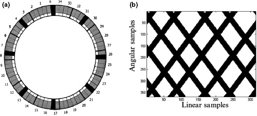
(a) A PET scanner configuration consisting of 35 detector modules where 8 blocks were turned off (black) to simulate missing detector response; (b) Corresponding gap mask in the sinogram space; black lines corresponds to the removed detectors (images are from Ref. [14]).
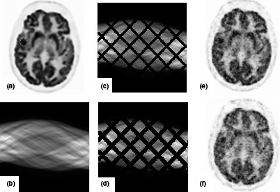
To evaluate how these methods, tolerate the amount of missing data, two gap structures referred to as small and large gap were simulated as shown in Figs. 3(c)–3(d) where 30% of data are missing for small gap and 48% for large gap. As shown in this figure, we have no data or noise in gap regions and our aim was to remove the noise from non‐gap regions and estimate data for gap regions as well.
Figure 3.
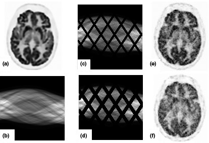
Display of patient brain phantom and reconstructed images; (a) brain phantom; (b) sinogram data; (c) noisy sinogram with small gap; (d) noisy sinogram with large gap; (e), (f) reconstructed images.
The algorithms used in this study include several parameters to needed to be properly set for the desired results. We carried out grid search on the parameters for each algorithm and parameters producing the best result were chosen. We have shown how the parameter selection affects the results for some of our methods in Data S1.
All data reconstruction was performed in 2D. All computations were executed with MATLAB R2015a using Core i7 CPU (3.60 GHz with 8 GB RAM, 64‐bit operating system).
3.B. Results for the patient brain phantom
Our first experiment was performed using brain images acquired using a whole‐body Discovery 690 PET/CT (GE Healthcare, Milwaukee, USA). These data were reconstructed using the HOTV‐PAPA as described in Ref. 46. The brain phantom image was reconstructed on a 256 × 256 matrix and a field of view of 300 mm (pixel size = 1.1718 × 1.1718 mm).
Figure 3 depicts our data and simulated noisy sinograms with two gap structures. Regarding the noise level, we have done experiments with three noise levels in this section. However, we only show the figures for medium noise level where the number of counts for low noise level is 1.11 × 10⁷ and 8.03 × 10⁶; for medium noise level is 4.45 × 10⁶ and 3.21 × 10⁶; for high noise level is 2.22 × 10⁶ and 1.60 × 10⁶ for small and large gap simulations, respectively. In the following subsections to show the efficiency of the methods for missing data recovery, we first show the results of OSEM reconstruction after modeling the gap structure in the PET scanner system matrix [A in Eq. (9)] in this figure. The low quality of the images and the presence of artifacts shown in Fig. 3 highlights the problems associated with uneven sampling in the sinograms.
3.B.1. Inpainting results
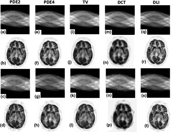
In this section, the performance of various inpainting methods including second‐ and fourth‐order PDEs1 (Eqs. (1) and (2) respectively), TV regularization2 [Eq. (6)], DCT‐based penalized regularization3 [Eq. (7)], and sparse DLI4 [Eq. (8)] is presented. Figure 4 illustrates the qualitative inpainting results using the different approaches mentioned above. In this figure, results of inpainting for small and large simulated gaps are shown in the first and third rows, respectively. Following the inpainted sinograms, we have shown the results of reconstructions by OSEM (second and forth rows) for comparison to the different inpainting methods.
Figure 4.
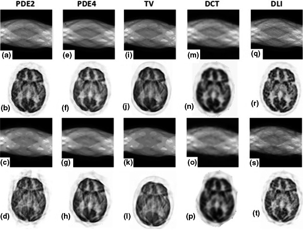
Inpainting results for patient brain phantom on medium noise level; (a–d) results of PDE2; (e–h) results of PDE4; (i–l) results of TV; (m–p) results of DCT; (q–t) results of DLI. First row: inpainted sinograms for small gap; second row: reconstructed images from first row; third row: inpainted sinograms for large gap; fourth row: reconstructed images from third row.
The results of inpainting algorithms used in this study depend on the number of iterations. As such, we report the results after the change of the cost function falls below a threshold of 10−7 between successive updates. For more information, the interested reader is referred to our Data S1.
Comparing the results of second‐ and fourth‐order PDEs (shown in first and second column of Fig. 4) reveals that the curvature of the equipotential lines is not preserved by PDE2 technique, which was expected because they are connected by a straight line across the missing domain. This phenomenon is more visible for large gap experiment where it manifests as blocky structures in PDE2's sinogram data. Additionally, Figs. 4(a)–4(d) show that the equipotential lines might be disconnected across large distances, which lead to undesirable images. This problem is moderately solved by PDE4 technique as shown in Figs. 4(e)–4(h).
The inpainting results using the TV regularization as depicted in Figs. 4(i)–4(l) show “staircase” artifacts (piecewise constant regions that form steps along gradients in the image) in sinogram image which are more visible in the presence of large gap. In more complex images (as shown in next sections), the finer details of them may not be acceptably recovered.
DCT‐based penalized inpainting technique‐based results are shown in Figs. 4(m)–4(p). Because this method was specifically formulated to smooth data, the blurring artifacts are unavoidable with this approach.27
Figures 4(q)–4(t) shows the DLI results. We observed that in the absence of Poisson noise, the method works well for gap filling task where some previous issues such as linear interpolation of equipotential lines or smoothness artifacts are not observed anymore. However, in the presence of noise, the results were considerably degraded. The method used for DLI can effectively recover the missing part of the data, but unable to simultaneously remove the Poisson noise from the non‐gap portions of the sinogram.
For quantitative comparison, one can refer to Table 1, where we compare the methods in terms of RMSE, SSIM, and computation time for three noise levels. We used a grid search to optimize the parameters for each method (see Data S1, Tables S1 and S2). Since the ground truth in image space is known, RMSE and SSIM have been measured in image space and are reported in Table 1. As shown, for low and medium noise levels, DLI approach outperforms the other methods in terms of RMSE and SSIM for both small and large gaps but at considerably more computational cost. For high noise level, DLI results are superior to others in case of small gap, but PDE4 performs better than DLI in case of large gap simulation and needed much less computation time.
Table 1.
Results of different inpainting approaches for patient brain phantom study; RMSE and SSIM values are given in image space
| Method | Low noise level | Medium noise level | High noise level | Time (s) | |||||||||
|---|---|---|---|---|---|---|---|---|---|---|---|---|---|
| Small gap | Large gap | Small gap | Large gap | Small gap | Large gap | ||||||||
| RMSE | SSIM | RMSE | SSIM | RMSE | SSIM | RMSE | SSIM | RMSE | SSIM | RMSE | SSIM | ||
| PDE2 | 11.08 | 95.98 | 13.92 | 93.07 | 11.57 | 95.72 | 15.09 | 92.77 | 12.24 | 94.86 | 14.43 | 92.06 | 22.35 |
| PDE4 | 10.32 | 96.06 | 13.04 | 93.56 | 11.54 | 95.89 | 15.04 | 92.78 | 11.44 | 95.41 | 14.08 | 92.68 | 23.31 |
| TV | 15.12 | 92.35 | 16.31 | 92.15 | 16.32 | 92.34 | 17.20 | 92.14 | 17.20 | 90.75 | 17.52 | 90.41 | 85.14 |
| DCT | 13.05 | 94.40 | 14.36 | 92.24 | 13.13 | 94.04 | 15.08 | 91.74 | 13.40 | 93.91 | 15.12 | 91.69 | 19.68 |
| DLI | 8.06 | 97.81 | 12.24 | 94.28 | 9.09 | 97.45 | 13.02 | 93.55 | 11.04 | 96.98 | 14.13 | 92.55 | 621.35 |
The bold values refer to the best values among the methods.
3.B.2. Compressed sensing results
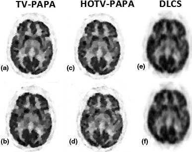
Using the simulated partial sampling, three different CS‐based reconstruction approaches (TV‐PAPA, HOTV‐PAPA, and DLCS) have been evaluated in this section. The reconstruction results for two scenarios of small and large gap structures are depicted in Fig. 5.
Figure 5.
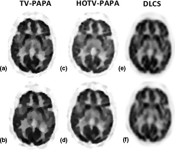
Compressed sensing results for the patient brain phantom on medium noise level; (a), (b) reconstructed image from TV‐PAPA for small and large gap, respectively; (c), (d) reconstructed image from HOTV‐PAPA for small and large gap, respectively; (e), (f) reconstructed image from DL for small and large gap, respectively.
Figure 5 shows that HOTV‐PAPA outperforms TV‐PAPA. DL based reconstruction although improves the quality of reconstructed images with respect to no compensation, it still produces poor results comparing to other CS‐based approaches.
Table 2 shows the quantitative results of the methods as well as their execution time. As shown, HOTV‐PAPA outperforms to others in terms of RMSE and SSIM. The execution time for HOTV‐PAPA is very close to TV‐PAPA.
Table 2.
Results of different compressed sensing approaches for brain phantom study; RMSE and SSIM values are given in image space
| Method | Low noise level | Medium noise level | High noise level | Time (s) | |||||||||
|---|---|---|---|---|---|---|---|---|---|---|---|---|---|
| Small gap | Large gap | Small gap | Large gap | Small gap | Large gap | ||||||||
| RMSE | SSIM | RMSE | SSIM | RMSE | SSIM | RMSE | SSIM | RMSE | SSIM | RMSE | SSIM | ||
| TV‐PAPA | 10.65 | 97.64 | 12.50 | 95.13 | 11.73 | 97.15 | 13.03 | 93.09 | 11.78 | 96.47 | 13.55 | 92.24 | 29.53 |
| HOTV‐PAPA | 10.29 | 97.77 | 12.14 | 95.15 | 11.15 | 97.34 | 12.28 | 94.10 | 11.64 | 96.51 | 13.18 | 94.05 | 30.84 |
| DLCS | 17.28 | 79.45 | 17.93 | 77.62 | 19.27 | 78.44 | 19.96 | 77.06 | 20.32 | 76.68 | 21.15 | 72.55 | 689.12 |
The bold values refer to the best values among the methods.
3.C. Results for the patient derived abdomen phantom
The second part of our experiments was also performed using images acquired using a whole‐body Discovery 690 PET/CT (GE Healthcare, Milwaukee, USA). The images were acquired from a patient nominally injected with 370 MBq and scanned 1‐h postinjection 3 min per bed position. The reconstruction was performed using GE VuePoint FX OSEM with sharpIR using 2 × 28 (iterations/subsets) and a 6.4 mm FWHM transaxial post filter. The abdomen image was reconstructed on a 256 × 256 matrix and a field of view of 700 mm (2.734 mm pixels).
Figure 6 displays one slice (abdomen part) of the whole‐body scan and its projected 2D sinogram. Again, to show the efficiency of the methods for missing data recovery in the following subsections, the reconstruction results of noisy and under sampled simulated data for two gap structures are shown in this figure. In this study, we only simulated medium level of noise with 2.66 × 10⁶ and 1.64 × 10⁶ counts for small and large gap simulations respectively.
Figure 6.
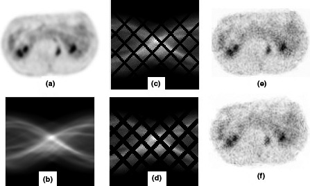
Display of the patient abdomen phantom and reconstructed images; (a) abdomen slice of whole‐body scan; (b) sinogram data; (c) noisy sinogram with small gap; (d) noisy sinogram with large gap; (e), (f) reconstructed images by OSEM.
3.C.1. Inpainting results
The results of all inpainting approaches for both small and large gap structures are depicted in Fig. 7. The columns of the figure respectively depict the results of PDE2, PDE4, TV, DCT, and DLI. First and third rows show inpainted sinograms for small and large gap structures respectively, while the results of reconstruction by OSEM are depicted in second and forth rows.
Figure 7.
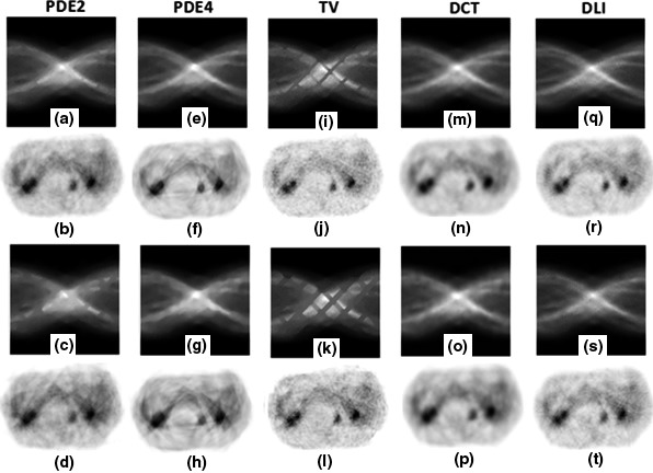
Inpainting results for the patient abdomen phantom on medium noise level; (a–d) results of PDE2; (e–h) results of PDE4; (i–l) results of TV; (m–p) results of DCT; (q–t) results of DL. First row: inpainted sinograms for small gap; second row: reconstructed images from first row; third row: inpainted sinograms for large gap; fourth row: reconstructed images from third row.
Table 3 shows the quantitative results which are quite comparable. DLI approach is superior to others in both terms of RMSE and SSIM.
Table 3.
Results of different inpainting approaches for the patient abdomen phantom; RMSE and SSIM values are given in image space
| Method | Medium noise level | |||
|---|---|---|---|---|
| Small gap | Large gap | |||
| RMSE | SSIM | RMSE | SSIM | |
| PDE2 | 8.31 | 93.69 | 8.36 | 91.55 |
| PDE4 | 6.66 | 96.97 | 7.42 | 93.73 |
| TV | 8.56 | 93.02 | 9.63 | 90.60 |
| DCT | 9.36 | 96.76 | 10.40 | 92.64 |
| DLI | 5.17 | 97.93 | 6.86 | 94.91 |
The bold values refer to the best values among the methods.
3.C.2. Compressed sensing results
Figure 8 shows the results of compressed sensing based image reconstruction for both small and large gap structures. The columns show the results for TV‐PAPA, HOTV‐PAPA, and DLCS, respectively. The results of small gap are depicted in first row, while the second row shows the results of large gap structure. For qualitative comparison, the results of HOTV‐PAPA are superior to others.
Figure 8.
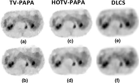
Compressed sensing results for the patient abdomen phantom on medium noise level; (a), (b) reconstructed image from TV‐PAPA for small and large gap, respectively; (c), (d) reconstructed image from HOTV‐PAPA for small and large gap, respectively; (e), (f) reconstructed image from DLCS for small and large gap, respectively.
The quantitative results are tabulated in Table 4. The best RMSE and SSIM values belong to HOTV‐PAPA.
Table 4.
Results of different compressed sensing approaches for the patient abdomen phantom; RMSE and SSIM values are given in image space
| Method | Medium noise level | |||
|---|---|---|---|---|
| Small gap | Large gap | |||
| RMSE | SSIM | RMSE | SSIM | |
| TV‐PAPA | 6.94 | 96.92 | 7.12 | 95.28 |
| HOTV‐PAPA | 5.69 | 97.92 | 6.61 | 96.45 |
| DLCS | 15.13 | 92.54 | 17.72 | 89.75 |
The bold values refer to the best values among the methods.
3.D. Lesion simulation
For lesion simulation on brain phantom data, we first consider a circle of radius 3 pixels (3.52 mm), and add the mean activity of that region to the lesion pixel values as shown in Fig. 9.
Figure 9.
Display of patient brain phantom with simulated lesion and reconstructed images; (a) brain phantom; (b) sinogram data; (c) noisy sinogram with small gap; (d) noisy sinogram with large gap; (e), (f) reconstructed images.
We have also investigated the performance of the methods using simulated lesion with contrast recovery coefficient (CRC)47 as following
| (14) |
where is the true contrast in the original simulated lesion before adding gap structure and noise, while is the measured contrast after reconstruction. S and B are the intensity of lesion and background respectively.
Like Section 3.B, we again simulated three noise levels where the count numbers are 1.12 × 10⁷ and 8.09 × 10⁶ for low noise level, 4.48 × 10⁶ and 3.23 × 10⁶ for medium noise level, and 2.24 × 10⁶ and 1.61 × 10⁶ for high noise level, for small and large gap structures, respectively. Figures 10 and 11 show the qualitative results of inpainting and CS‐based reconstruction only for medium noise level, while Tables 5 and 6 tabulate the quantitative results. To compare the results in term of RSME/SSIM, one can refer to Data S1 (Figs. S5 and S6, Tables S3 and S4). In term of CRC, DLI and HOTV performances are the best for small and large gap simulations, respectively.
Figure 10.
Inpainting results for patient brain phantom with simulated lesion on medium noise level; (a–d) results of PDE2; (e–h) results of PDE4; (i–l) results of TV; (m–p) results of DCT; (q–t) results of DLI. First row: inpainted sinograms for small gap; second row: reconstructed images from first row; third row: inpainted sinograms for large gap; fourth row: reconstructed images from third row.
Figure 11.
Compressed sensing results for the patient brain phantom; (a), (b) reconstructed image from TV‐PAPA for small and large gap, respectively; (c), (d) reconstructed image from HOTV‐PAPA for small and large gap, respectively; (e), (f) reconstructed image from DL for small and large gap, respectively.
Table 5.
CRC results for different inpainting approaches for patient brain phantom study with lesion simulation
| Method | Low noise level | Medium noise level | High noise level | |||
|---|---|---|---|---|---|---|
| Small gap | Large gap | Small gap | Large gap | Small gap | Large gap | |
| PDE2 | 76.24 | 75.16 | 74.57 | 73.08 | 74.11 | 70.54 |
| PDE4 | 77.68 | 76.49 | 77.43 | 75.31 | 74.63 | 74.93 |
| TV | 65.09 | 60.84 | 63.58 | 59.02 | 63.24 | 59.00 |
| DCT | 76.28 | 70.72 | 75.95 | 70.19 | 72.28 | 70.06 |
| DLI | 84.85 | 77.93 | 84.55 | 76.95 | 80.92 | 75.19 |
The bold values refer to the best values among the methods.
Table 6.
CRC results of different compressed sensing approaches for brain phantom study with simulated lesion
| Method | Low noise level | Medium noise level | High noise level | |||
|---|---|---|---|---|---|---|
| Small gap | Large gap | Small gap | Large gap | Small gap | Large gap | |
| TV‐PAPA | 80.13 | 76.38 | 80.30 | 78.00 | 78.45 | 72.09 |
| HOTV‐PAPA | 82.90 | 82.56 | 84.22 | 79.85 | 78.85 | 75.21 |
| DLCS | 70.29 | 62.88 | 60.52 | 59.46 | 60.23 | 53.48 |
The bold values refer to the best values among the methods.
4. Discussion
In this work, we investigated the effectiveness of recently developed methodologies for image inpainting and artifact reduction in reduced view PET imaging. To do this we used two different images from patients to create simulated data with two levels of gap structure, we evaluated and compared implementation of gap filling techniques directly in sinogram space vs. compensation of missing data adjoined with reconstruction, as to which is more effective to preserve the quality and quantitative accuracy of the recovered images.
In our studies, the quantitative results (as shown in Data S1, Figs. [Link], [Link], [Link], for better comparison) show that DLI outperforms other methods for small gap though having relatively high computational cost. For large gap structure, HOTV‐PAPA produces better results.
Our evaluation of noise effect on performance of approaches indicates that in case of low and medium noise levels, DLI still produces better results among inpainting approaches; however for the high noise level the performance of DLI degrades. This occurs because, at lower noise (higher counts), Poisson noise approximates Gaussian noise, while at higher noise (lower counts), the Poisson nature of the data is evident. While the DLI method is very successful at removing Gaussian noise, it does not remove Poisson noise well. On the other hand, HOTV‐based compressed sensing performs favorably for high noise levels because it penalizes first‐ and second‐order gradients, helping to preserve the piecewise‐linear aspects of the data.
The inpainting methods presented in this study do not account for the data consistency issues, which may be more problematic with larger gaps. Our interest in using inpainting techniques stems from its extensive development in the image processing community; more so than compressed sensing methods. Indeed, projection data lend itself very naturally to 2D image processing techniques. In addition, the optimization of the inpainting problems is simpler than compressed sensing methods. For these reasons, especially in the case of small gaps where data inconsistency is smaller, sinogram inpainting methods may perform better than simpler compressed sensing techniques such as TV (or HOTV). However, as the results show, this breaks down as the gaps get larger.
For images with texture, the inpainting approaches such as DLI or PDE4 may be more appropriate. DLI method does not encounter issues such as linear interpolation of equipotential lines or smoothness artifacts. However, if the computational time is critical, PDE4 may be a candidate replacement. The main drawback of PDE2 is that the equipotential lines are interpolated linearly. Therefore, the curvatures of lines are not preserved, which may result in straight line connections across the missing domain that may produce unsatisfactory outcome in the presence of large gap. However this problem is moderately solved by PDE4.
Because of staircase artifacts associated with first‐order TV‐based inpainting method, it is more suitable for recovery piecewise constant images. DCT on the other hand, because it produces blurring artifacts, favors globally smooth activity distributions and will not faithfully reproduce edges.
As inferred from above, the performance of the various methods is influenced by the characteristics of the images (e.g., TV and Piecewise constant images). As a result, our examination of these methods using just two types of PET images, brain and abdomen, is not exhaustive and other activity distributions may give different results. However, we note that though the brain and abdomen are very different images, the results were consistent with one another, which is encouraging.
In future work, we wish to apply the techniques to projection data from a PET scanner with partial geometry for further assessment. In addition to finding the best technique for estimating missing data, investigating the optimal detector gap configuration in a PET scanner which leads to satisfactory recovery results will be very useful in scanner design for special applications.
5. Conclusion
In conclusion, the results using the images in this study suggest that CS‐based reconstruction approaches like HOTV‐PAPA can more effectively improve the quality of recovered images especially where a large portion of data is missing. In the case of smaller gaps, the inpainting methods are more competitive and can perform similarly to the compressed sensing approaches used in this study. It was demonstrated that one may utilize the extra information from inpainting techniques, as obtained at the position of missing data in the projection space, which could lead to improved reconstruction.
Conflict of interest
The authors have no conflicts to disclose.
Supporting information
Fig. S1: Inpainting results for patient brain phantom on medium noise level; First row: mean results for small gap; second row: standard deviation results for small gap; third row: mean results for large gap; fourth row: standard deviation results for large gap.
Fig. S2: Compressed sensing results for patient brain phantom on medium noise level; First row: mean results for small gap; second row: standard deviation results for small gap; third row: mean results for large gap; fourth row: standard deviation results for large gap.
Fig. S3: Inpainting results for the patient abdomen on medium noise level; First row: mean results for small gap; second row: standard deviation results for small gap; third row: mean results for large gap; fourth row: standard deviation results for large gap.
Fig. S4: Compressed sensing results for the patient abdomen phantom on medium noise level; First row: mean results for small gap; second row: standard deviation results for small gap; third row: mean results for large gap; fourth row: standard deviation results for large gap.
Fig. S5: Inpainting results for patient brain phantom with simulated lesion on medium noise level; First row: mean results for small gap; second row: standard deviation results for small gap; third row: mean results for large gap; fourth row: standard deviation results for large gap.
Fig. S6: Compressed sensing results for the patient brain phantom on medium noise level; First row: mean results for small gap; second row: standard deviation results for small gap; third row: mean results for large gap; fourth row: standard deviation results for large gap.
Fig. S7: Comparison of the methods in terms of RMSE and SSIM for brain phantom data.
Fig. S8: Comparison of the methods in terms of RMSE and SSIM for abdomen phantom data.
Fig. S9: Comparison of the methods in terms of RMSE and SSIM and CRC for brain phantom data with simulated lesion.
Table S1: Results of parameter setting for TV‐based inpainting for large gap simulation in brain phantom study (RMSE at the first line, SSIM at the second line).
Table S2: Results of parameter setting for TV‐PAPA for large gap simulation in brain phantom study.
Table S3: Results of different inpainting approaches for patient brain phantom study with lesion simulation; RMSE and SSIM values are given in image space.
Table S4: Results of different compressed sensing approaches for patient brain phantom study with lesion simulation; RMSE and SSIM values are given in image space.
Data S1: Recovery of missing data in partial geometry PET scanners: Compensation in projection space vs image space.
Acknowledgments
This research was supported by Iran's National Elites Foundation, as well as Research Center for Molecular and Cellular Imaging at the Tehran University of Medical Sciences under grant number 94‐04‐165‐31062. It was also funded in part through the National Institutes of Health/National Cancer Institute Cancer Center support grant number P30 CA008748.
Notes
The source code for PDE‐based inpainting is available at: http://www.mathworks.com/matlabcentral/fileexchange/34356-higher-order-total-variation-inpainting
The source code for TV‐based inpainting is available at: https://github.com/gpeyre/2011-TIP-tv-projection
The source code for DCT‐based inpainting is available at: http://www.mathworks.com/matlabcentral/fileexchange/27994-inpaint-over-missing-data-in-1-d--2-d--3-d--n-d-arrays
The source code for nonparametric Bayesian dictionary learning is available at: http://people.ee.duke.edu/~mz1/
References
- 1. Rahmim A, Zaidi H. PET versus SPECT: strengths, limitations and challenges. Nucl Med Commun. 2008;29:193–207. [DOI] [PubMed] [Google Scholar]
- 2. Wahl R. Principles and Practice of PET and PET/CT. Philadelphia, USA: Lippincott Williams and Wilkins; 2008. [Google Scholar]
- 3. Kadrmas DJ, Christian PE. Comparative evaluation of lesion detectability for 6 PET imaging platforms using a highly reproducible whole‐body phantom with 22Na lesions and localization ROC analysis. J Nucl Med. 2002;43:1545–1554. [PubMed] [Google Scholar]
- 4. Kanade SS, Gujare SS. Comparative study of different digital inpainting algorithms. IJECET. 2014;5:258–265. [Google Scholar]
- 5. Bertalmio M, Sapiro G. Image inpainting. In: 27th International Conference on Computer Graphics and Interactive Techniques Conference. Los Angeles: ACM Press; 2000:417–424. [Google Scholar]
- 6. Criminisi A, Toyama K. Region filling and object removal by exemplar‐based image inpainting. IEEE Trans Image Proc. 2004;13:1–13. [DOI] [PubMed] [Google Scholar]
- 7. Rane SD, Sapiro G, Bertalmio M. Structure and texture filling‐in of missing image blocks in wireless transmission and compression applications. IEEE Trans Image Proc. 2003;12:296–303. [DOI] [PubMed] [Google Scholar]
- 8. Chen Y, Li Y, Guo H, et al. CT metal artifact reduction method based on improved image segmentation and sinogram in‐painting. Math Probl Eng. 2012;2012:1–18. [Google Scholar]
- 9. Abdoli M, Dierckx RAJO, Zaidi H. Metal artifact reduction strategies for improved attenuation correction in hybrid PET/CT imaging. Med Phys. 2012;39:3343–3360. [DOI] [PubMed] [Google Scholar]
- 10. Candes EJ, Wakin MB. An introduction to compressive sampling. IEEE Signal Process Mag. 2008;21:21–30. [Google Scholar]
- 11. Lu H, Wei J, Liu Q, Wang Y, Deng X. A dictionary learning method with total generalized variation for MRI reconstruction. Int J Biomed Imaging. 2016;2016:1–13. [DOI] [PMC free article] [PubMed] [Google Scholar]
- 12. Li S, Cao Q, Chen Y, Hu Y. Dictionary learning based sinogram inpainting for CT sparse reconstruction. Opt Int J Light Electron Opt. 2014;125:2862–2867. [Google Scholar]
- 13. Valiollahzadeh S, Clark JW, Mawlawi O. Using compressive sensing to recover images from PET scanners with partial detector rings. Med Phys. 2015;42:121–133. [DOI] [PMC free article] [PubMed] [Google Scholar]
- 14. Valiollahzadeh S, Clark JW, Mawlawi O. Dictionary learning for data recovery in positron emission tomography. Phys Med Biol. 2015;60:5853–5871. [DOI] [PMC free article] [PubMed] [Google Scholar]
- 15. Tauber Z, Li Z, Drew MS. Review and preview: disocclusion by inpainting for image‐based rendering. IEEE Trans Syst Man Cybern. 2007;37:527–540. [Google Scholar]
- 16. Qin C, Wang S, Zhang X. Simultaneous inpainting for image structure and texture using anisotropic heat transfer model. Multimedia Tools Appl. 2012;56:469–483. [Google Scholar]
- 17. Chan TF, Shen J. Variational image inpainting. Commun Pure Appl Math. 2005;58:579–619. [Google Scholar]
- 18. Burger M, He L, Schonlieb C‐B. Cahn‐hilliard inpainting and a generalization for grayvalue images. SIAM J Imaging Sci. 2009;2:1–25. [Google Scholar]
- 19. Bertozzi A, Esedoglu S, Gillette A. Inpainting of binary images using the Cahn‐Hilliard equation. IEEE Trans Image Proc. 2007;16:285–291. [DOI] [PubMed] [Google Scholar]
- 20. Schonlieb C, Bertozzi A. Unconditionally stable schemes for higher order inpainting. Commun Math Sci. 2011;9:413–457. [Google Scholar]
- 21. Rudin LI, Osher S, Fatemi E. Nonlinear total variation based noise removal algorithms. Phys D. 1992;60:259–268. [Google Scholar]
- 22. Chan TF, Golub GH, Mulet P. A nonlinear primal‐dual method for total variation‐based image restoration. SIAM J Sci Comput. 1995;20:1–11. [Google Scholar]
- 23. Goldfarb D, Yin W. Second‐order cone programming methods for total variation‐based image restoration. SIAM J Sci Comput. 2005;27:622–645. [Google Scholar]
- 24. Vogel CR, Oman ME. Iterative methods for total variation denoising. SIAM J Sci Comput. 1996;17:1–13. [Google Scholar]
- 25. Fadili JM, Peyre G. Total variation projection with first order schemes. IEEE Trans Image Proc. 2011;20:657–669. [DOI] [PubMed] [Google Scholar]
- 26. Wang G, Garcia D, Liu Y, De JR, Dolman AJ. A three‐dimensional gap filling method for large geophysical datasets: application to global satellite soil moisture observations. Environ Model Softw. 2012;30:139–142. [Google Scholar]
- 27. Garcia D. Robust smoothing of gridded data in one and higher dimensions with missing values. Comput Stat Data Anal. 2010;54:1167–1178. [DOI] [PMC free article] [PubMed] [Google Scholar]
- 28. Pati Y, Rezaiifar R, Krishnaprasad P. Orthogonal matching pursuit: recursive function approximation with applications to wavelet decomposition. In: Signals, Systems and Computers. Proceedings of 27th Asilomar Conference on Signals, Systems and Computers, IEEE, Pacific Grove, CA; 1993. [Google Scholar]
- 29. Chen SS, Donoho DL, Saunders MA. Atomic decomposition by basis pursuit. SIAM Rev. 2001;43:129–159. [Google Scholar]
- 30. Blumensath T, Davies ME. Iterative hard thresholding for compressed sensing. Appl Comput Harmon Anal. 2009;27:265–274. [Google Scholar]
- 31. Shojaeilangari S, Yau W, Nandakumar K, Li J, Teoh EK. Robust representation and recognition of facial emotions using extreme sparse learning. IEEE Trans Image Proc. 2015;24:2140–2152. [DOI] [PubMed] [Google Scholar]
- 32. Aharon M, Elad M, Bruckstein A. K‐SVD: an algorithm for designing overcomplete dictionaries for sparse representation. IEEE Trans Signal Process. 2006;54:4311–4322. [Google Scholar]
- 33. Mairal J, Bach F, Ponce J. Task‐driven dictionary learning. IEEE Trans Pattern Anal Mach Intell. 2012;43:791–804. [DOI] [PubMed] [Google Scholar]
- 34. Zhou M, Chen H, Paisley J, Ren L, Sapiro G, Carin L. Non‐parametric Bayesian dictionary learning for sparse image representations. IEEE Trans Image Proc. 2012;21:1–9. [DOI] [PMC free article] [PubMed] [Google Scholar]
- 35. Li S, Zhang J, Krol A, et al. Effective noise‐suppressed and artifact‐reduced reconstruction of SPECT data using a preconditioned alternating projection algorithm. Med Phys. 2015;42:4872–4887. [DOI] [PMC free article] [PubMed] [Google Scholar]
- 36. Krol A, Li S, Shen L, Xu Y. Preconditioned alternating projection algorithms for maximum a posteriori ECT reconstruction. Inverse Probl. 2012;28:115005. [DOI] [PMC free article] [PubMed] [Google Scholar]
- 37. Boyd S, Parikh N, Chu E, Peleato B, Eckstein J. Distributed optimization and statistical learning via the alternating direction method of multipliers. Found Trends Mach Learn. 2011;3:1–122. [Google Scholar]
- 38. Chambolle A, Pock T. A first‐order primal‐dual algorithm for convex problems with applications to imaging. J Math Imaging Vis. 2011;40:120–145. [Google Scholar]
- 39. Lange K, Carson R. EM reconstruction algorithms for emission and transmission tomography. J Comput Assist Tomogr. 1984;8:306–316. [PubMed] [Google Scholar]
- 40. Shepp LA, Vardi Y. Maximum likelihood reconstruction for emission tomography. IEEE Trans Med Imaging. 1982;1:113–122. [DOI] [PubMed] [Google Scholar]
- 41. Hudson HM, Larkin RS. Accelerated image reconstruction using ordered subsets of projection data. IEEE Trans Med Imaging. 1994;13:100–108. [DOI] [PubMed] [Google Scholar]
- 42. Wang Z, Bovik AC, Sheikh HR, Member S, Simoncelli EP, Member S. Image quality assessment: from error visibility to structural similarity. IEEE Trans Image Proc. 2004;13:1–14. [DOI] [PubMed] [Google Scholar]
- 43. Bosch J, Stoll M. A fractional inpainting model based on the vector‐valued Cahn–Hilliard. SIAM J Imaging Sci. 2015;8:2352–2382. [Google Scholar]
- 44. Berthon B, Häggström I, Apte I, et al. PETSTEP: generation of synthetic PET lesions for fast evaluation of segmentation methods. Phys Med Eur J Med Phys. 2015;31:969–980. [DOI] [PMC free article] [PubMed] [Google Scholar]
- 45. Häggström I, Beattie B, Schmidtlein C. Dynamic PET simulator via tomographic emission projection for kinetic modeling and parametric image studies. Med Phys. 2016;43:3104–3116. [DOI] [PMC free article] [PubMed] [Google Scholar]
- 46. Schmidtlein C, Lin Y, Li S, et al. Relaxed ordered subset preconditioned alternating projection algorithm for PET reconstruction with automated penalty weight selection. Med Phys. 2017;44:4083–4097. [DOI] [PMC free article] [PubMed] [Google Scholar]
- 47. Hsu C. A study of lesion contrast recovery for iterative PET image reconstructions versus filtered backprojection using an anthropomorphic thoracic phantom. Comput Med Imaging Graph. 2002;26:119–127. [DOI] [PubMed] [Google Scholar]
Associated Data
This section collects any data citations, data availability statements, or supplementary materials included in this article.
Supplementary Materials
Fig. S1: Inpainting results for patient brain phantom on medium noise level; First row: mean results for small gap; second row: standard deviation results for small gap; third row: mean results for large gap; fourth row: standard deviation results for large gap.
Fig. S2: Compressed sensing results for patient brain phantom on medium noise level; First row: mean results for small gap; second row: standard deviation results for small gap; third row: mean results for large gap; fourth row: standard deviation results for large gap.
Fig. S3: Inpainting results for the patient abdomen on medium noise level; First row: mean results for small gap; second row: standard deviation results for small gap; third row: mean results for large gap; fourth row: standard deviation results for large gap.
Fig. S4: Compressed sensing results for the patient abdomen phantom on medium noise level; First row: mean results for small gap; second row: standard deviation results for small gap; third row: mean results for large gap; fourth row: standard deviation results for large gap.
Fig. S5: Inpainting results for patient brain phantom with simulated lesion on medium noise level; First row: mean results for small gap; second row: standard deviation results for small gap; third row: mean results for large gap; fourth row: standard deviation results for large gap.
Fig. S6: Compressed sensing results for the patient brain phantom on medium noise level; First row: mean results for small gap; second row: standard deviation results for small gap; third row: mean results for large gap; fourth row: standard deviation results for large gap.
Fig. S7: Comparison of the methods in terms of RMSE and SSIM for brain phantom data.
Fig. S8: Comparison of the methods in terms of RMSE and SSIM for abdomen phantom data.
Fig. S9: Comparison of the methods in terms of RMSE and SSIM and CRC for brain phantom data with simulated lesion.
Table S1: Results of parameter setting for TV‐based inpainting for large gap simulation in brain phantom study (RMSE at the first line, SSIM at the second line).
Table S2: Results of parameter setting for TV‐PAPA for large gap simulation in brain phantom study.
Table S3: Results of different inpainting approaches for patient brain phantom study with lesion simulation; RMSE and SSIM values are given in image space.
Table S4: Results of different compressed sensing approaches for patient brain phantom study with lesion simulation; RMSE and SSIM values are given in image space.
Data S1: Recovery of missing data in partial geometry PET scanners: Compensation in projection space vs image space.


