Shrinkage observed-to-expected ratios for robust and transparent large-scale pattern discovery

Abstract

Large observational data sets are a great asset to better understand the effects of medicines in clinical practice and, ultimately, improve patient care. For an empirical pattern in observational data to be of practical relevance, it should represent a substantial deviation from the null model. For the purpose of identifying such deviations, statistical significance tests are inadequate, as they do not on their own distinguish the magnitude of an effect from its data support. The observed-to-expected (OE) ratio on the other hand directly measures strength of association and is an intuitive basis to identify a range of patterns related to event rates, including pairwise associations, higher order interactions and temporal associations between events over time. It is sensitive to random fluctuations for rare events with low expected counts but statistical shrinkage can protect against spurious associations. Shrinkage OE ratios provide a simple but powerful framework for large-scale pattern discovery. In this article, we outline a range of patterns that are naturally viewed in terms of OE ratios and propose a straightforward and effective statistical shrinkage transformation that can be applied to any such ratio. The proposed approach retains emphasis on the practical relevance and transparency of highlighted patterns, while protecting against spurious associations.

1 Introduction

In exploratory analysis of observational medical data, many patterns of potential interest correspond to variations in event rates. Medical diagnoses, drug prescriptions and laboratory test results are all viewed naturally as discrete events. Sets of events may occur together more often (or rarely) than expected, or a given event may be unusually common or rare in a specific region, time period or age group, for example. The identification of excess co-reporting of certain suspected adverse drug reactions (ADRs) with specific medicines is at the core of post-marketing drug safety surveillance based on individual case safety reports.^1,2 Several public health and individual patient safety issues have been first highlighted with statistical pattern discovery in this data.^3,4 Recently, there has been increased interest in pattern discovery also for longitudinal patient records and medical claims.

Conceptually, patterns can be characterised as local structures that generate data with an anomalously high (or low) density relative to that expected under a global baseline model.⁵ In the context of this article, we focus on the specific class of patterns that can be defined as contrasts between an observed and an expected number of events. The expected number is computed under an appropriate baseline model, and the choice of baseline model varies with the type of pattern under consideration. For pairs of events, the baseline model may be that events occur independently of one another; for measures of interaction, the baseline model may take into account lower order associations between pairs of events; and for patterns of temporal association a simple baseline model may be that the association between two events may be constant over person time.

An important consideration in selecting the measure of association for a given pattern discovery application is its relative emphasis on the strength of association versus the amount of data support. Measures based exclusively on statistical significance focus primarily on data support and are prone to highlighting weak associations of limited practical relevance.² The observed-to-expected (OE) ratio, on the other hand, focuses exclusively on the strength of association, but is volatile when the observed or expected numbers of events are low (in particular if the expected count is much lower than one). Shrinkage is a statistical approach to regularise a measure through moderation towards a null value, in the absence of enough data to support a deviation. For OE ratios, shrinkage towards 1 (no deviation) reduces the risk of highlighting spurious assocations while it retains emphasis on the practical relevance of any highlighted patterns. It has proven an effective compromise in a single measure between the strength of association and amount of data support in large-scale pattern discovery.² Shrinkage OE ratios have been used routinely for over a decade in pattern discovery of ADR surveillance data,¹ and have been shown useful in other applications including the analysis of international telephone call data.⁶ A key rate limiter for their widespread adoption may have been the technical complexity of currently available shrinkage transformations, such as the complex set of priors in Norén et al.⁷ and the bimodal five parameter prior distribution in DuMouchel² which can be challenging to implement, and hard to interpret for those responsible to clinically assess highlighted patterns. In contrast, we have recently implemented shrinkage OE ratios for higher order interactions⁸ and temporal pattern discovery⁹ using a simple shrinkage transformation which is more transparent and can be computed at the back of an envelope. In this article, we propose broader use of the simple shrinkage transformation and outline a range of patterns that are naturally viewed in terms of OE ratios.

2 OE ratios

Many measures of association for pattern discovery can be expressed in terms of contrasts between an observed number of events, and the expected number of events under an appropriate baseline model. In this section, we describe OE ratios for pairwise association, higher order interaction and temporal association. We also discuss how adjustment by stratification can eliminate the undue impact of other covariates on the OE ratio of interest, and the importance of visualisation.

2.1 Pairwise association

Most measures in large-scale pattern discovery are for pairwise association. This is true also for patterns involving more than two events, when the measure of association is based on grouping the events into two distinct subsets (e.g. a pairwise association between a medical diagnosis and the co-prescription of two drugs). Assume the following contingency table based on a cross-classification of database records according to whether or not they involve the two sets of events of interest x and y:

$$\begin{array}{c}\multicolumn{1}{c}{\begin{array}{c}\hfill \text{y not}\hspace{1em}\text{y}\hfill \\ \multicolumn{6}{c}{}\\ \multicolumn{1}{c}{\text{x}ab}\\ \multicolumn{1}{c}{\text{not}\hspace{1em}\text{x}cd}\end{array}}\\ \multicolumn{1}{c}{\mathrm{vrule}}\end{array}$$

A simple OE ratio for the association between x and y relative to an independence baseline model can be computed based on the ratio of f(y ∣ x), the relative frequency of y conditional on the occurrence of x, to f(y), the marginal relative frequency of y (or vice versa, the measure is symmetrical in x and y):

$$f(\text{y x})f(\mathbf{\text{y}})=a/(a+b)(a+c)/(a+b+c+d)$$ (1)

It can be re-expressed as an OE ratio for the number of events:

$$\text{OE}=\text{a}(\text{a}+\text{b})·(\text{a}+\text{c})/(\text{a}+\text{b}+\text{c}+\text{d})$$ (2)

Relative risk-type measures such as the Proportional Reporting Ratio¹⁰ provide a more distinct contrast between the observed and expected numbers of events by comparing f(y ∣ x) to the relative frequency of y in the absence of x: f(y ∣ not x):

$$\text{PRR}=\text{f}(\mathbf{\text{y x}})\text{f}(\text{y not x})=\text{a}/(\text{a}+\text{b})\text{c}/(\text{c}+\text{d})$$ (3)

Re-expression in terms of an OE ratio is straightforward:

$$\text{OE}=\text{a}(\text{a}+\text{b})·\text{c}/(\text{c}+\text{d})$$ (4)

An important limitation of (2) and (4) is that their ranges of possible values depend on the marginal frequencies of the events of interest. By definition, (1) cannot exceed 1/f(x) or 1/f(y) and (3) cannot exceed 1/f(y ∣ not x). As a consequence, events with high marginal frequencies cannot yield high OE ratios, which makes these measures primarily useful for rare events and unsuitable as a basis for comparing the strength of association across events with substantially different marginal frequencies.

The odds ratio is an alternative measure of association which can be estimated as:

$$\text{OR}=\text{f}(\text{y x})/(1-\mathbf{\text{f}}(\text{y x}))\text{f}(\text{y not x})/(1-\mathbf{\text{f}}(\text{y not x}))=\text{ad bc}$$ (5)

The odds ratio has many desirable properties for a measure of association.¹¹ Specifically, it is variation independent of the marginal frequencies f(x) and f(y ), and thus applies equally well to common and rare events. The odds ratio is easily re-expressed in terms of an OE ratio:

$$\text{OE}=\text{a b}·\text{c}/\text{d}$$ (6)

For this OE ratio, the expected count is computed under the assumption that the odds of y are unaffected by x, and vice versa. Such an analysis requires conditioning on the exact contingency table counts b, c and d, rather than the marginals. One disadvantage of the odds ratio is that it is undefined when b or c are zero. Upon re-expression as in (6), its expected count is undefined when d is zero. This will rarely be an issue in database-wide analyses of rare events but could be problematic under stratification as described in Section 2.5.

A simple illustration of the types of patterns that can be identified with pairwise OE ratios are provided in Table 1, which lists the countries with most extreme OE ratios according to (2) for the reporting rates of chest pain in the WHO Global Individual Case Safety Reports Database, VigiBase.¹² The interpretation of the observed variation across countries is far from straightforward and would require a more in-depth analysis considering, for example, population demographics, coding practices and regulations for reporting.

Table 1.

Country variation in the reporting of chest pain in the WHO Global Individual Case Safety Reports database, VigiBase, as identified with OE ratios compared to a simple independence model

Country	Observed	Expected	OE
United States	56116	41466	1.35
Canada	5729	4442	1.29
Singapore	337	265	1.27
…
Romania	11	100	0.11
Tunisia	6	70	0.09
Cuba	38	512	0.07

2.2 Contrasts

Contrasts expressed as ratios between OE ratios are OE ratios in their own right:

$${\text{OE}}_{\Delta }=\text{OE}″\text{OE}=\text{O}″\text{O}·\text{E}″\text{E}$$ (7)

This is an attractive property that allows more sophisticated measures of association to be constructed. These derived OE ratios can be subjected to the same statistical shrinkage transformation, adjustment by stratification and visualisation, as simple OE ratios. They can be an effective basis to screen for variation in the strength of association across data subsets, and more specifically for interactions and temporal associations as described in Sections 2.3 and 2.4.

2.3 Interaction

The measures in Section 2.1 are for pairwise association only (whether between individual events or sets of events). Measures of interaction identify patterns of event co-occurrence that indicate an effect on the strength of association between two (sets of) events by a third (or more) event or covariate. Interaction can be measured as an OE ratio where the expected value is based on a regression model without the interaction term of interest.⁶ Alternatively, interaction can be defined as a ratio of the pairwise OE ratio for x and y conditional on a third event z to the unconditional OE ratio for x and y (the measure is symmetrical in x, y and z).⁷ For the OE ratio in (2):

$${\text{OE}}_{\mathbf{\text{xyz}}}={\text{OE}}_{\mathbf{\text{xyz}}}{\text{OE}}_{\mathbf{\text{xy}}}={\text{O}}_{\mathbf{\text{xyz}}}{\text{E}}_{\mathbf{\text{xyz}}}{·}_{\text{O}}\text{xy}/\text{E}\text{xy}=\dots ={\text{n}}_{\text{xyz}}({\text{n}}_{\text{xy}}·{\text{n}}_{\text{xz}}·{\text{n}}_{\text{yz}}·\text{n})/({\text{n}}_{\text{x}}·{\text{n}}_{\text{y}}·{\text{n}}_{\mathbf{\text{z}}})$$ (8)

Here, n denotes the total number of records in the data set, n_xyz the number of records on which x, y and z occur together, and so forth. Extensions to even higher order associations are possible too.⁷

Interaction as defined in (8) and with standard regression-based approaches, such as log-linear models and logistic regression, use a baseline model in which the individual effects of x and y on z essentially multiply in the absence of interaction. This will not always be appropriate, in particular when the individual effects are of considerable magnitude. As an alternative, the expected count can be computed under a baseline model of additive increases in the rate of z due to each of x and y.⁸ A schematic illustration of such a baseline model is provided in Figure 1. In this case, the expected count is based on the absolute excess in the rate of z attributable to the independent effects of x and y. Unlike (8), such third-order OE ratios are not symmetrical in x, y and z, but will depend on the assumed direction of the potential interaction (in this case x and y interact to cause z).

Figure 1.

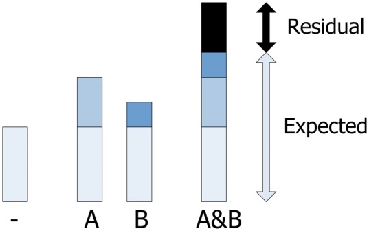
Schematic overview of an interaction between two conditions A and B relative to an additive baseine model. The bars correspond to the frequency of the event of interest (1) in the absence of both A and B, (2) with A but not B, (3) with B but not A, and (4) with A and B together. The shades correspond to: the marginal relative frequency of the event (lightest), the increased frequency attributable to A, the increased frequency attributable to B, and the increased frequency attributable to an interaction between A and B (darkest).

To illustrate the difference between these two types of baseline models for interaction detection, consider an event that is twice as common for women as for men, and twice as common for those above 65 years of age as for those below 65. In this case, the additive model predicts that the event should be approximately three times (1+(2−1)+(2−1)) as common for women above age 65 as for men below age 65 in the absence of interaction. Baseline models such as that for (8) on the other hand predict that the event should be approximately four times (1 · 2 · 2) as common for women above 65 years of age, because the relative risks essentially multiply for rare events. The additive baseline model has clear advantages as a basis for both individual decision-making and public policy-making.¹³ Moreover, empirical results suggest that it is better suited to detect some patterns indicative of adverse drug interactions, at least in individual case safety reports.⁸

2.4 Temporal association

Temporal patterns relating the occurrence of one event to another in time are of interest in the analysis of longitudinal patient records and medical claims. Elevated rates of a medical diagnosis relative to the prescription of a certain medicine may indicate a safety issue (if subsequent to prescription) or an indication for treatment (if prior to prescription). Lowered rates of a medical diagnosis can reflect beneficial effects (if subsequent to prescription) or contra-indications (if prior to prescription). Similarly, associations over time in the prescription of different medicines relative to one another may represent switching patterns. A framework for temporal pattern discovery in longitudinal observational databases based on OE ratios has previously been described.⁹ It computes OE ratios for the number of times that one event (x) is followed by another event (y) in different time periods. The expected number of events y in each time period relative to x is based on the overall rate of y in the same time period relative to other events in an external control group (for example prescriptions of other medicines). While OE ratios in a specific time period could in principle provide the basis for large-scale pattern discovery, a contrast between two OE ratios as discussed in Section 2.2 has proven more effective.⁹ Simultaneous consideration of separate time periods allows for a distinction between true temporal association and underlying tendencies of two events to occur in the same patients. The proposed measure contrasts the OE ratio for y relative to x in a time period of interest v to the corresponding OE ratio between y and x in a pre-defined control period u:

$${\text{OE}}^{\text{vu}}={\text{O}}^{\text{v}}{\text{E}}^{\text{v}}·{\text{O}}^{\text{u}}/{\text{E}}^{\text{u}}$$ (9)

The baseline model accommodates time-constant associations between the two events of interest, but stipulates that the OE ratio be the same in the time period of interest v, as in the control period u. Deviations suggest that there is an association between the two events in the time period of interest beyond their overall association across these patient histories. This OE ratio controls for both the baseline frequency of y relative to x and for the overall temporal association between y and events in the control group. By appropriate selection of time periods u and v, a wide variety of classes of temporal patterns can be screened for.⁹

Traditional epidemiological designs can be leveraged to yield sophisticated OE ratios for the purpose of exploratory analysis, beyond the methodology described here. For example, some measures from cohort and self-controlled designs are directly interpretable as OE ratios and can be subjected to statistical shrinkage in order to provide robust but relevant effect measures in pattern discovery for patient records and medical claims.

2.5 Adjustment by stratification

In the analysis of observational data, events or covariates other than those of primary interest may distort the association under scrutiny. An association between a childhood vaccine and abnormal crying might, for example, be driven by the fact that both events are common in young children. Indeed, there may be no association, or an association in the opposite direction, if different age groups are studied separately. This is an example of confounding. Stratification is a simple but transparent approach to reduce the negative impact of suspected confounding by analysing subsets (as specified by the suspected confounders) of the data separately. An overall OE ratio adjusted for suspected confounders can be obtained as a weighted average of stratum-specific OE ratios in which the OE ratio for each subset is weighted by the corresponding expected number of events E in that stratum.^2,7,14

$$\text{OE}=\sum _{\text{j}=1}^{\text{m}}({\text{O}}_{\text{j}}/{\text{E}}_{\text{j}})·{\text{E}}_{\text{j}}\sum _{\text{j}=1}^{\text{m}}{\text{E}}_{\text{j}}=\text{O}\sum _{\text{j}=1}^{\text{m}}{\text{E}}_{\text{j}}$$ (10)

Note that the expression simplifies to a modified OE ratio in which the overall expected count in (11) is replaced by a sum over the expected counts in each subset j. Adjustment by stratification does assume that the OE ratio is constant across strata, which will not always hold. This may require stratum-specific OE ratios be quoted instead. Moreover, caution must be exercised in order not to stratify by too many covariates at once. The analysis is carried out conditional on the expected counts in every single stratum, and very small strata can happen to have substantial but untrustworthy expected counts. Empirical results show that the presence of any very small strata may lead to spurious under-estimation of thus adjusted OE ratios.¹⁴

2.6 Visualisation

Shrinkage OE ratios are a natural basis for visualisation. They are especially powerful in combination with information on the underlying observed and expected counts, as these counts provide a direct link to the empirical basis of any observed pattern.

At the core of the temporal pattern discovery methods for patient records in Norén et al.⁹ is a graphical statistical approach to visualising temporal association, referred to as the chronograph. Figure 2 provides an example from the analysis of electronic patient records. Its upper panel plots the log OE ratio with uncertainty intervals (subjected to the shrinkage transformation to be introduced in Section 3.1) for diagnoses of swelling in different time periods relative to prescriptions of an antihypertensive medicine. The lower panel depicts the corresponding observed and expected numbers of events. An asterisk depicts the rates for the day of the first prescription.

Figure 2.

Visualisation of OE ratios over time, for the association in a collection of electronic patient records between first prescriptions of an antihypertensive medicine and diagnoses of swelling. The top panel displays the logarithm of the OE ratio (with shrinkage) over time. The bottom panel displays the underlying observed and expected numbers of events. Reproduced from Norén et al. [9] with permission from Springer.

The shrinkage OE ratio in the upper panel of the chronograph compensates for some systematic variability that may otherwise distort the analysis: it is not biased by the greater tendency of medical events to be recorded if they occur close in time to a prescription, or of truncation and censoring,⁹ as reflected by a peak in the expected number of events around time 0 in Figure 2. The lower panel of the chronograph is more sensitive to systematic variability but highlights absolute differences between the observed and expected, and provides direct insight into the empirical basis for the upper graph. While limited to a specific pair of events, the chronograph spans a multitude of time intervals before and after the index event, x. It can be a great support in the clinical assessment of highlighted patterns. A consistently high OE ratio throughout the chronograph suggests a general tendency for event y to occur in the same event histories as event x. A transient increase in the OE ratio for event y immediately prior to event x may indicate that y triggers x. Similarly, an increase in the OE ratio for y immediately after x may indicate that x triggers y. However, temporal associations do not necessarily imply causality, as there are a number of possible explanations for why one event may tend to occur soon after the other.

Figure 3 provides another visualisation of OE ratios – in this instance for the association between fluoxetine and neonatal withdrawal syndrome in the WHO Global Individual Case Safety Reports database, VigiBase. It illustrates the evolution over time as data accumulates on this safety issue first highlighted in Sanz et al.³

Figure 3.

Visualisation of the retrospective evolution over time of the OE ratio for the association between fluoxetine and neonatal withdrawal syndrome in the WHO Global Individual Case Safety Reports database, VigiBase. The top panel displays the logarithm of the OE ratio (with shrinkage) over time. The bottom panel displays the underlying observed and expected numbers of events.

3 Shrinkage

Statistical shrinkage is the regularisation of an estimate by evaluating several parameters simultaneously or by combining data with external information or assumptions. It is inherent in the Bayesian approach to statistical inference, where the posterior distribution provides a compromise between the observed data likelihood and an assumed prior distribution. However, shrinkage estimators were first proposed by Stein and colleagues as an approach to achieve lower quadratic loss in frequentist analysis.¹⁵

From a practical perspective, shrinkage regularises a volatile measure by introducing a bias towards a null value in exchange for better variance properties. In large-scale pattern discovery, shrinkage of the OE ratio towards 1 provides protection against highlighting spurious associations. In Section 3.1, we present a simple shrinkage transformation applicable to any OE ratio. This transformation is a generalisation of the shrinkage previously applied to measures of interaction⁸ and temporal association.⁹ Like the EBGM measure, it is based on a Gamma-Poisson model,² but it uses a much simpler parametric form and allows, but does not require empirical Bayes re-estimation. It combines observed data with a prior assumption that the baseline model used to compute the expected count holds. For a given choice of parameter values, its properties are very similar to those of the more complex shrinkage transformations previously proposed for the IC measure.^1,7

3.1 Simple shrinkage transformation

Consider an OE ratio with observed number of events O and expected number of events E. Let the analysis be carried out conditional on E. We propose the following simple shrinkage transformation:

$$O+{\alpha }_{1}E+{\alpha }_2$$ (11)

The addition of α₁ to the nominator and α₂ to the denominator provides shrinkage towards an OE ratio of α₁/α₂. Setting α₁ = α₂ results in shrinkage towards 1 corresponding to no discrepancy between the observed and the expected. Such shrinkage provides a conservative measure of association with reduced volatility less prone to highlight spurious associations, in particular for events with very low expected frequency. In general, the impact of this shrinkage is equivalent to that of α₁ additional observed events, and α₂ additional expected events. The strength and the direction of the shrinkage can easily be adjusted by altering the magnitude of α₁ and α₂ and their ratio, respectively. As the observed and expected number of events increase, the impact of the shrinkage diminishes.

Formally, (11) can be viewed as the Bayeisan posterior mean of a parameter μ under the assumption that O is Poisson Po(μ · E)-distributed with a Gamma prior distribution for μ: G(α₁, α₂). Based on the Gamma G(α₁, α₂) prior distribution, the posterior distribution for μ will also be Gamma (but with parameters O + α₁ and E + α₂). Bayesian credibility intervals (an alternative to frequentist confidence intervals) can be computed that indicate a range of values compatible with the data at hand. For μ, the credibility interval limits correspond to percentiles of the Gamma distribution with parameters O + α₁ and E + α₂. They can be computed with standard statistical software as the inverse of the Gamma cumulative distribution function. As the analysis is carried out conditional on the expected value E, it is important to choose a baseline model that provides reasonably precise expected values.

The logarithm of the OE ratio is a convenient measure of association in the sense that its sign indicates the direction of the association and its magnitude measures the strength of positive and negative associations on comparable scales – for the base 2 logarithm, every unit shift corresponds to a doubling or halving of the OE ratio. The above shrinkage transformation extends directly, so that shrunk log₂ OE ratios can be computed as:

$${\log }_{2}O+{\alpha }_{1}E+{\alpha }_2$$ (12)

The corresponding credibility interval limits are log₂ μ_q. For back-of-the-envelope calculations, the following expression (a simplified version of the formula proposed in Norén et al.⁷) provides an approximate lower limit of a two-sided 95% interval for (12):

$${\log }_{2}O+{\alpha }_{1}E+{\alpha }_2-3.3·(O+{\alpha }_1{)}^{-1/2}-2·(O+{\alpha }_1{)}^{-3/2}$$ (13)

A corresponding expression for the upper limit is:

$${\log }_{2}O+{\alpha }_{1}E+{\alpha }_2+2.4·(O+{\alpha }_1{)}^{-1/2}-0.5·(O+{\alpha }_1{)}^{-3/2}$$ (14)

The loss in accuracy of (13) and (14) is in the second decimal relative to the exact solutions based on the inverse of the Gamma cumulative distribution function, as long as the observed count plus α₁ exceeds 1. For uncertainty intervals around log OE ratios when the observed count is 0, the exact uncertainty limits above should be used (unless α₁ is greater than or equal to 1).

An approximate similarity between (12) with α₁ = α₂ = 1 and an earlier implementation of the IC measure of association¹ was first suggested by DuMouchel.² Indeed, one can show that for data sets with at least 1000 records, a recent update of the IC measure of association⁷ is very well approximated by (12) with α₁ = α₂ = 1/2; even for very small data sets, the discrepancy is only in the second decimal.

3.2 Variations

The appropriate choice of α₁ and α₂ will vary depending on the application. Higher α₁ and α₂ values provide stronger protection against highlighting spurious associations, and an α₁/α₂ ratio other than 1 will provide shrinkage towards a different null value, which may be motivated if there is prior information to suggest that two events are associated one way or the other (such as perhaps information from a pre-approval randomised controlled trial).

As an alternative to manually selecting the α values, an empirical Bayes approach can be used in which the prior distribution is fitted to the empirical distribution of unshrunk OE ratios for a large set of event pairs.² With such an approach, the prior will vary with the data set to be analysed, and will also vary for a given data set as it evolves over time. Some implementations have included only event pairs with observed counts greater than or equal to 1 in the fitting of the prior distribution,² but this will bias the prior towards higher values, since true negative associations are more likely than true positive associations to result in zero counts. If used as a basis for empirical Bayes estimation, the simple prior distribution in Section 3.1 will be easy to fit, robust to fluctuations in data (see the discussion of hyper-parameter identifiability in DuMouchel²) and allow for a direct interpretation of the fitted parameters in terms of the strength and the direction of the shrinkage. The one-component Gamma distribution may not always fit the empirical distribution of OE ratios as well as the more flexible two-component Gamma distribution used in DuMouchel,² but this can be expected to have limited practical impact relative to the other distortions in large-scale pattern discovery in observational data.

4 Discussion

Patterns of pairwise association, higher order interaction, and temporal association, can all be quantified in terms of OE ratios. The OE ratio is conceptually intuitive and reflects the extent to which an observed pattern deviates from the assumed baseline model. Large relative differences between the observed and the expected tend to signify patterns of practical importance, and the OE ratio can be useful for comparing strength of association across different data subsets. A fundamental limitation of raw OE ratios is that they are sensitive to random variability. They are particularly volatile when the expected number of events is low, which is problematic for applications such as drug safety surveillance in which rare events can be critically important.² Statistical shrinkage reduces the negative impact of artificially low expected counts, and stabilises the OE ratio in their presence. In combination with uncertainty intervals, it reduces the risk of highlighting spurious associations. It does not explictly account for the multiple comparisons inherent in large-scale pattern discovery and will not control the familywise Type 1 error rate (the probability of any false positive finding) or the false discovery rate (FDR).^16–18 Two methods for large-scale pattern discovery based on shrinkage OE ratios with direct reference to the FDR have been proposed.^16,18 One uses the posterior probability that an observation has been drawn from the extreme component of a mixture of two Gamma distributions¹⁶ and the other uses the posterior probability that the OE ratio exceeds a given threshold.¹⁸ The former requires a mixture prior distribution, whereas the latter implements the same Bayesian decision rule as presented here: a threshold for posterior percentiles of the shrinkage OE ratio. However, in terms of ranking potential patterns for consideration, both FDR-based approaches focus on the probability that a pattern represents a chance findings, rather than on the magnitude of the deviation between the observed and expected. Like statistical significance tests, they do not on their own convey the practical relevance of different patterns. This reduces their usefulness as a basis for exploratory analysis as in the identification of outstanding reporting patterns in Table 1. The FDR-based approaches may be a competitive alternative as binary decision rules for targeted surveillance – in particular when there is a substantial premium for false alerts. In the context of exploration, and in particular if early discovery is a main priority, the down-prioritisation of strong associations with limited data support can be inappropriate. The FDR below 0.05 reported in a recent simulation study for decision rules based on common thresholds and percentiles of shrinkage OE ratios unadjusted for multiple comparisons¹⁸ provides some reassurance that the method proposed here does not generate a large proportion of spurious associations. Of course, such FDRs as those mentioned above must be interpreted with caution since they reflect only random variability and do not account for the biases and confounders ever present in observational data. Statistical significance tests rely on the accurate account of all sources of variability (both random and systematic),¹⁹ and so does effective pattern discovery. Related to this, one should bear in mind that the uncertainty intervals provided in Section 3.1 account for random but not systematic variability and provide a measure of precision but not accuracy. Moreover, they are computed under the assumption that data points are independent and, therefore, they may exaggerate the precision of an OE ratio in the presence of clustered data points.

The absence of a complex statistical superstructure for the shrinkage transformation in Section 3.1 is a clear advantage over the computationally more sophisticated alternatives in Bate et al.,¹ DuMouchel² and Norén et al.⁷ The simple form of (11) retains a clear link to the underlying OE ratio, and makes explicit the reliance on the underlying baseline model. To further emphasise the importance of the empirical basis for highlighted patterns, we recommend that observed and expected numbers of events always accompany quoted OE ratios, as in the graphical displays of Figures 2 and 3. This reduces the risk that the shrinkage transformation diverts domain experts from careful consideration of alternative explanations to outstanding quantitative associations. As an example, in the presence of suspected duplicate data points that contribute to an observed count,²⁰ simple arithmetics will indicate to what extent duplication can explain a large OE ratio, whereas more complex methods may require the entire analysis to be repeated.²¹

That said, there are patterns for which the OE ratio is not the most appropriate measure of association. For example, the practical relevance of highlighted patterns might in some applications be better measured in terms of absolute differences between the observed and expected numbers of events.⁶ Confounding is a fundamental challenge in the analysis of observational data. Adjustment by stratification can under certain circumstances reduce the unwanted impact of a limited number of suspected confounders, as outlined in Section 2.5. However, it is most suitable for categorical variables, whereas for numerical covariates a discretisation is required that can be delicate and sometimes inappropriate. Moreover, adjustment by stratification is only appropriate in the absence of effect modification and is not feasible in the presence of moderate to large numbers of suspected confounders. Methods such as propensity scores that reduce the dimensionality of the suspected confounders can potentially offer some relief in those circumstances. Shrinkage regression is an alternative approach that has been successfully applied to the analysis of individual case safety reports in the presence of confounding by co-reported medicines.^22,23 Its main advantage is that it can incorporate a large number of suspected confounders simultaneously and can naturally accommodate both discrete and numerical covariates. Its efficiency stems from the underlying model's assumptions of linearity (on some scale), which may not always be fulfilled. Regardless of the method for adjustment, confounding by unmeasured covariates remains a potential source of mis-interpretation that should always be considered in the analysis of outstanding reporting patterns.

There are clear advantages of using the same shrinkage OE ratio as the basis for a broad range of pattern discovery applications, as proposed in this article. It allows experience of the shrinkage transformation for one OE ratio to be benefited from by another. As highlighted in Section 2.1, the odds ratio can be re-expressed as an OE ratio and subjected to the simple shrinkage transformation in Section 3, thus adding effective protection against spurious associations to its list of desirable properties. Similarly, the adjustment by stratification first proposed for pairwise associations in DuMouchel² can be directly applied to the measure of interaction in Norén et al.⁸ or to the temporal pattern discovery framework in Norén et al.⁹

References

- 1.Bate A, Lindquist M, Edwards IR, et al. A Bayesian neural network method for adverse drug reaction signal generation. Eur J Clin Pharmacol 1998; 54: 315–321. [DOI] [PubMed] [Google Scholar]
- 2.DuMouchel W. Bayesian data mining in large frequency tables, with an application to the FDA spontaneous reporting system. Am Stat 1999; 53: 177–202. [Google Scholar]
- 3.Sanz EJ, De-las-Cuevas C, Kiuru A, Bate A, Edwards IR. Selective serotonin reuptake inhibitors in pregnant women and neonatal withdrawal syndrome: a database analysis. Lancet 2005; 365: 482–487. [DOI] [PubMed] [Google Scholar]
- 4.Edwards IR, Bate A, Lindquist M. Abacavir and increased risk of myocardial infarction. Lancet 2008; 372(9641): 805–805. [DOI] [PubMed] [Google Scholar]
- 5.Hand DJ, Bolton R. Pattern Discovery and Detection: A Unified Statistical Methodology. J Appl Stat 2004; 31(8): 885–924. [Google Scholar]
- 6.DuMouchel W, Pregibon D. Empirical Bayes screening for multi-item associations. 2001. KDD '01: Proceedings of the Seventh ACM SIGKDD International Conference on Knowledge Discovery and Data Mining, CA: San Francisco, pp. 67–76. [Google Scholar]
- 7.Norén GN, Bate A, Orre R, Edwards IR. Extending the methods used to screen the WHO drug safety database towards analysis of complex associations and improved accuracy for rare events. Stat Med 2006; 25(21): 3740–3757. [DOI] [PubMed] [Google Scholar]
- 8.Norén GN, Sundberg R, Bate A, Edwards IR. A statistical methodology for drug–drug interaction surveillance. Stat Med 2008; 27(16): 3057–3070. [DOI] [PubMed] [Google Scholar]
- 9.Norén GN, Hopstadius J, Bate A, Star K, Edwards IR. Temporal pattern discovery in longitudinal electronic patient records. Data Mining Knowledge Discov 2010; 20(3): 361–387. [Google Scholar]
- 10.Evans SJW, Waller PC, Davis S. Use of proportional reporting ratios (PRRs) for signal generation from spontaneous adverse drug reaction reports. Pharmacoepidemio. Drug Saf 2001; 10(6): 483–486. [DOI] [PubMed] [Google Scholar]
- 11.Tan P, Kumar V, Srivastava J. Selecting the right interestingness measure for association patterns. 2002. KDD '02: Proceedings of the Eighth ACM SIGKDD International Conference on Knowledge Discovery and Data Mining, New York, NY, USA: ACM, pp. 32–41. [Google Scholar]
- 12.Lindquist M. VigiBase, the WHO global ICSR database system: basic facts. Drug Inf J 2008; 42: 409–419. [Google Scholar]
- 13.Rothman KJ, Greenland S, Walker AM. Concepts of interaction. Am J Epidemiol 1980; 112(4): 467–470. [DOI] [PubMed] [Google Scholar]
- 14.Hopstadius J, Norén GN, Bate A, Edwards IR. Adjustment for potential confounders in adverse drug reaction surveillance. Drug Saf 2008; 31(11): 1035–1048. [DOI] [PubMed] [Google Scholar]
- 15.James W, Stein J. Estimation with quadratic loss. In: Neyman J. (ed.) Proceedings of the Third Berkeley Symposium on Mathematical Statistics and Probability Berkeley, CA: University of California Press, 1961, pp. 361–379. [Google Scholar]
- 16.Gould AL. Accounting for multiplicity in the evaluation of ‘signals’ obtained by data mining from spontaneous report adverse event databases. Biometric J 2007; 49(1): 151–165. [DOI] [PubMed] [Google Scholar]
- 17.Webb GI. Discovering significant patterns. Mach Learn 2007; 68(1): 1–33. [Google Scholar]
- 18.Ahmed I, Thiessard F, Miremont-Salamé G, Bégaud B, Tubert-Bitter P. Pharmacovigilance data mining with methods based on false discovery rates: a comparative simulation study. Clin Pharmacol Ther 2010; 88(4): 492–498. [DOI] [PubMed] [Google Scholar]
- 19.Cox DR. Statistical significance tests. Br J Clin Pharmacol 1982; 14(3): 325–331. [DOI] [PMC free article] [PubMed] [Google Scholar]
- 20.Norén GN, Orre R, Bate A, Edwards IR. Duplicate detection in adverse drug reaction surveillance. Data Mining Knowledge Discov 2007; 14: 305–328. [Google Scholar]
- 21.Hauben M, Madigan D, Hochberg AM, Reisinger SJ, O'Hara DJ. Data mining in pharmacovigilance: computational cost as a neglected performance parameter. Int J Pharm Med 2007; 21(5): 319–323. [Google Scholar]
- 22.Genkin A, Lewis DD, Madigan D. Large-scale Bayesian logistic regression for text categorization. Technometrics 2007; 49(3): 291–304. [Google Scholar]
- 23.Caster O, Norén GN, Madigan D, Bate A. Large-scale regression-based pattern discovery: the example of screening the WHO global drug safety database. Stat Anal Data Mining 2010; 3(4): 197–208. [Google Scholar]