Price of disorder in the Lac Repressor hinge helix

Abstract

The Lac system of genes has been pivotal in understanding gene regulation. When the lac repressor protein binds to the correct DNA sequence, the hinge region of the protein goes through a disorder to order transition. The structure of this region of the protein is well understood when it is in this bound conformation, but less so when it is not. Structural studies show that this region is flexible. Our simulations show this region is extremely flexible in solution; however, a high concentration of salt can help kinetically trap the hinge helix. Thermodynamically, disorder is more favorable without the DNA present.

Graphical Abstract

1. Introduction

The lactose repressor (LacI) regulates the expression of a set of genes involved in lactose metabolism in the bacterium Escherichia coli. LacI was one of the first gene-regulatory proteins discovered¹ and is well studied.² The structure has been determined to have four main regions: the tetramerization region (TR), regulatory domain (RD), hinge-helix linker region (HH), and DNA-binding domain (DBD)³, shown in Figure 1. Although the protein is well studied, the region of the HH is still poorly understood in terms of its importance in the DNA recognition process.^{4, 5} In particular, questions about thermodynamic and kinetic control exist.

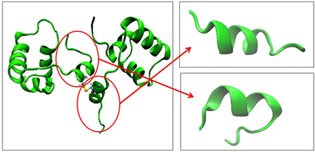
Fig 1.

LacI repressor protein bound to operator DNA. Image created using PDB 2pe5.

Atomic structures of the protein bound to DNA in non-specific and specific complexes are available from crystallographic and nuclear magnetic resonance experiments^6–8. These structures show that the 9 amino acid long HH is disordered when it binds to non-specific DNA, but it changes to a helical conformation when bound to operator DNA. NMR and Molecular Dynamics (MD) studies have found that 6 of the 9 residues directly interact with the DNA through hydrogen bonds with the phosphate backbone (ASN50, GLN54), insertion into the minor groove (ALA53, LEU56, ALA57)⁹, or polar interactions (ASN50, ARG51)¹⁰.Other studies indicate the structure of this region, when unbound, is highly flexible or dynamic^{4, 5, 9, 11–14}. This linker region is disordered when unbound. Some proteins and protein domains do not have a well-defined structure in solution but instead may obtain structure only in a specific functional state. Such proteins, called intrinsically disordered or unstructured proteins, were first characterized in the mid-1990s and have been extensively studied ^15–26. The transition of this HH in LacI from unstructured to a helix coincides with binding a specific sequence of DNA. Coupled folding upon binding is not uncommon among proteins ^27–31.

Current theoretical techniques are challenged in describing proteins when in these disordered states, even though there has been much progress^{8, 9, 11, 32–37}. Informatics studies have discovered which amino acid sequences are more likely to be disordered^{16, 37}, how often disordered regions are found in proteins^{18, 24}, and common functions of these disordered proteins^{16, 22, 24}. It is, however, difficult to predict or measure the ensemble of geometric shapes. This inability to have a simple structural characterization of the hinge region of the lac repressor protein when unbound makes it interesting to understand the mechanism leading to the binding thermodynamics. The abundance of data^{2, 3, 5–11, 16, 25, 32–35, 38–81} available for the LacI protein makes it feasible to model some of the behavior of the system by means of computer simulation.

Here Molecular Dynamics (MD) simulations and advanced sampling methods were used to illuminate the underlying free energy surface governing the hinge region of the protein. The work presented in this contribution considered the role of the hinge helix in the context of the DNA binding domain and by itself. We considered the systems in both pure water and in a high salt solution to mimic the salt concentration found in the counterion condensed atmosphere near DNA where coupled folding and binding would occur. Straight forward simulations can lead to insufficient sampling of the helical and nonhelical states even when the system is reduced in complexity. To better understand this we sampled the free energy surface with metadynamics. The purpose of these calculations is to better understand the structural ensemble of the protein and corresponding energies when free in solution before considering the influence of DNA on the binding.

2. Methods

In order to consider the structural transitions of the HH region of LacI from the protein perspective (i.e. without DNA present) three strategies were employed. Because salt concentration is relatively high near DNA due to counterion condensation a salt concentration of 0.4M was included. Next the physical complexity of the system was reduced to see how the important HH subsystem on its own responded as a function of the saline environment. Finally the free energy surface along various collective variables was considered. The details of the systems are given in Table 1.

Table 1:

Description of simulations

Stage	Description of system	System Number	Simulation Technique	PDB Structure	Type of Water	Ion Concentration	Total # of atoms	Simulation Time
1	Full DNA binding domain and Hinge Helix (Residues 1-62) in solution “DBD+HH”	1	Classic MD	1CJG	TIP3P	.4M	56487	50ns
		2	Classic MD	1L1M	TIP3P	.4M	52159	1μs
		3	Classic MD	1OSL	TIP3P	.4M	47557	1μs
2	Single monomer, Hinge Helix only, in solution (Residues 50-62) “HH”	1	Classic MD	1L1M – mon. 1	TIP3P	.4M	10054	1μs
		2	Classic MD	1L1M – mon. 2	TIP3P	.4M	9519	1μs
		3	Classic MD	1OSL – mon. 1	TIP3P	.4M	10533	1μs
	Single monomer, Hinge Helix only, in solution (Residues 50-62) “HH”	4	Classic MD	1L1M – mon. 1	TIP3P	0M	10158	1μs
		5	Classic MD	1L1M – mon. 2	TIP3P	0M	9615	1μs
		6	Classic MD	1OSL – mon. 1	TIP3P	0M	10641	1μs
3	Single Monomer, Hinge Helix only, in solution (Residues 50-62) “HH”	1	Meta-dynamics	1L1M – mon. 1	TIP3P	.4M	10054	200ns
		2	Meta-dynamics	1L1M – mon. 1	TIP3P	0M	10154	150ns

2.1. Molecular Systems

To compare the differences between the ordered and disordered states of the HH region and avoid initial condition artifacts, MD simulations were performed starting in both states. Three stages of simulations were performed which are outlined in Table 1. Snapshots of each system can be found in Supplemental Figure 1. The first stage consisted of three simulations of the full homodimer DBD including the HH. The three systems of stage 1 were the ordered wild type (WT) DBD, ordered mutant DBD, and disordered mutant DBD. We performed the MD simulations starting from minimized crystal coordinates, discussed further below and in table 1, into the microsecond time scale. Stage 2 consisted of 6 simulations of a single monomer (monomer 1 or 2) of the HH region in varying ion concentrations also using crystal coordinates as starting structures. To explore the underlying free energy surface, Stage 3 consisted of two metadynamics simulations of a single monomer of the HH in different ion concentrations. For all stages of simulations, hydrogen atoms were added to the crystal structures using PSFGen in Visual Molecular Dynamics (VMD)⁸².

In stage 1 the ordered and disordered states of the full DBD (residues 1–62) were simulated. Current techniques are challenged to get a structure of the WT when in a disordered state, in solution or bound to a non-operator sequence. Because of this and to aid dimer formation, many previous experiments and simulations have been performed using either the PurR-GCG construct or the V52C mutant⁷⁵. The stage 1 systems were simulated starting from two of these V52C PDB structures, 1L1M⁸ and 1OSL⁸³. Both structures were dimers consisting of the first 62 N-terminal residues of each monomer, crystalized to operator and non-operator DNA respectively. As a control, the WT structure of the helical dimer, PDB code 1CJG⁷, was also simulated. The peptides were solvated in explicit TIP3P⁸⁴ water molecules. All 3 systems were simulated for 50ns with an ion concentration of .4M NaCl. The fluctuation of RMSD and radius of gyration along with energy components, including hydrogen bonds, were compared between the WT and mutant both starting in the helical conformation. No major differences were seen between the two ordered systems, 1CJG and 1L1M, so all remaining simulations were completed with one of the two mutants, either 1L1M or 1OSL. The two mutant DBD simulations were continued until they totaled 1μs.

Stage 2 was the investigation of only the HH region, residues 50–62. All 6 systems were neutrally capped with an acetyl group on the N-terminus and an N-methylamide on the C-terminus. Simulation 1 and 2 of stage 2 corresponded to monomer 1 and 2 of the 1L1M ordered structure respectively. Both were simulated at an ion concentration of 0.4M NaCl. Simulation 3 and 4 of stage 2 corresponded to monomer 1 and 2 of the 1L1M ordered structure respectively, both in a pure water solution. Simulation 5 of stage 2 included monomer 1 of the 1OSL disordered structure in an ion concentration of .4M NaCl. Simulation 6 of stage 2 included monomer 1 of the 1OSL disordered structure in a pure water solution. All stage 2 systems were simulated for 1μs each.

The third stage had two systems that started from the 1L1M ordered structure and captured aspects of the free energy surface of the RMS deviation of the HH from the crystal structure using metadynamics. Simulations 1 and 2 in stage 3 were of a single monomer of the HH region in high ion concentration and pure water respectively. These two HH systems were capped in the same manner as those in stage 2. System1 was sampled for a total of 150ns while System 2 was sampled for a total of 200ns.

2.2. Classical Molecular Dynamics

All molecular dynamics simulations were conducted using NAMD 2.10⁸⁵ and the CHARMM36 force field^{84, 86}. All systems were minimized for 21,000 steps then equilibrated for 640ps in an NVT ensemble at 300K. A weakly coupled Langevin thermostat⁸⁵ was used to maintain constant temperature. Electrostatic interactions were computed using the particle-mesh Ewald algorithm⁸⁷. The PME grid spacing was 1.0Å with a tolerance of 0.000001Å. The VMD package⁸² provided some analysis and visualization. As shown in table 1, most trajectories were continued to 1 μs.

2.3. Metadynamics

The free energy landscape representing the HH unfolding pathway was investigated by means of metadynamics⁸⁸ (3rd stage), an enhanced sampling method to calculate the free-energy surface as a function of a few selected collective variables (CVs). We tested a number of different collective variables including RMSD from the crystal structure, radius of gyration, end-to-end distance and helical content (see supplemental information). Each of these CV’s has desirable and undesirable characteristics⁸⁹. We used the root mean square deviation (RMSD) of residues 50–58 from the starting structure of each respective simulation as the CV and characterized helical content. The systems were run using NAMD 2.10⁸⁵ and the CHARMM36 force field^{84, 86}.

To begin metadynamics for systems 1 and 2, a Gaussian height of 1.0 kcal/mol was used. The systems were able to transit the entire range of the CV at least 5 times at the initial Gaussian height. The height was subsequently reduced as shown in table 2 to get a more accurate and smooth final PMF^{85, 90, 91}. For each subsequent height the systems traversed the entire range of the CV until the simulation showed regularity, at least 1trip/2ns (low ion) and 1trip/4ns (high ion), allowing for convergence. Every 50ps the NAMD program output a PMF file. Once all runs were complete, all pmfs from each Gaussian height were averaged using the block method (4 blocks/ns). Then every 4 points in energy were averaged. The average of the PMFs from the smallest height (0.3kcal/mol) are shown in Figure 4. The variance from the average PMFs for each height is shown in Supplemental Figure 5. The systems were then analyzed using VMD with plugins from PLUMED⁹², NAMD⁸⁵, and METAGUI⁹³ The cluster analysis using Metagui3.0 was used to cluster the metadynamics data based on RMSD. Once clustered, PLUMED was used to calculate the radius of gyration (atoms 1–134 aka residues 50–58), torsion angles of residues 51–58, and end-to-end distance (atoms 1–134) of each frame in those clusters. Using the 16 torsion angles of each frame, the number of consecutive helical residues (−90<φ<−35 and −70<ψ<−15 and −115<φ+ψ<−95)⁹⁴ was calculated. The metadynamics data was then reweighted using the original PMF and the populations of each variable per RMSD cluster.The reweighting followed the usual procedure for a biased distribution.

$$h_i^{\ast }=\frac{\sum _{j=0}^n{h}_i(x_j)e^{-\beta V(x_j)}}{\sum _{j=0}^{n}Q(x_j)e^{-\beta V(x_j)}}$$

where V(x_j) is the value of the original PMF at an RMSD of x_j, h_i(x_j) is the number of frames with the new CV at value i in RMSD cluster x_j, Q(x_j) is the bin size of the cluster at RMSD x_j and h_i* is the reweighted value for the new CV value for i.

Table 2:

Gaussian height changes over time in stage 3 metadynamics

System	Time @ 1.0 kcal/mol	@ 0.5 kcal/mol	@ 0.4 kcal/mol	@ 0.3 kcal/mol
Stage 3, System 1	10ns	20ns	50ns	120ns
Stage 3, System 2	10ns	10ns	30ns	100ns

Figure 4:

A,B) Graphs of the Potential of Mean Force during the single helix metadynamics simulations based on the collective variable of Root Mean Squared Deviation in high ion and low ion solutions respectively. C,D) For the high ion and low ion systems respectively, the % of residues in each RMSD cluster that were found to have a maximum length of consecutive helical residues corresponding to the colored legend (0 residues = purple, 1 residue = blue, 2 residues = teal, 3 residues = green, 4 residues = yellow, 5 residues = orange, 6 residues = red, 7 residues = maroon, 8 residues = black).

The reweighted PMFs are included in SF 9,10.

3. Results

3.1. Stage 1 Classical MD

Many have observed that the HH region of the peptide is dynamically disordered when free in solution^{4, 5, 9, 11–14}. To investigate this, the stage 1 simulations were performed starting from both ordered and disordered starting structures in order to observe what conformational changes occur during these reported fluctuations. The stage 1 simulation starting in the operator-bound (helix) conformation was found to be conformationally stable in the HH for the entire microsecond. In over half of the HH residues it was seen that they maintained their helical structure for over 90% of the time. (Figure 2) The ends of the helix frayed during the simulation, but those in the core remained helical. Thiswas unexpected for a very flexible system^{4, 5, 9, 11–14}. In the simulations starting from a disordered state, no helices were formed during the microsecond simulation which was not surprising. Exchange between the states was not well sampled (Supplemental Figure 2). Because the relaxation times could be greater than the simulation time no conclusions about the thermodynamic stability can be made from such calculations. The kinetic stability of these simulations could be coming from interactions with the rest of the DBD. Ions could affect the stability as well. To address both possibilities, we next considered the isolated HH and the effects of salt concentration.

Figure 2.

The time each individual residue spent in particular secondary structures throughout the full simulation. The dihedral angles for these structures were: Beta– phi=−180:−100, psi=120:180; RH Alpha Helix– phi=−138:−38, psi=−58:18; LH Alpha Helix – phi=38:88, psi=28:58 Beta was found to be present less than .15% of the time, and thus not included in the graph.

3.2. Stage 2 Classical MD

Stage 2 of the simulations explored systems containing only the HH in varying ion concentrations to explore the intrinsic characteristics of this subsystem. Short helices are rarely stable thermodynamically. We wished to explore the populations of conformations and the kinetics. When comparing the differences between systems 1–4 of stage 2, those that started in a helical structure in high ion concentrations versus those started in a helical structure with no ions, the ion concentration was found to have impact on the kinetic stability. Based on rules found by Zhang et al. for disorder in proteins^{19, 95}, this sequence of mostly small hydrophilic amino acids should favor disorder. Near the beginning of these simulations the systems were stable close to the starting structures with modest structural fluctuations. This stability was in evidence in the RMSD, end-to-end distance, and radius of gyration (see Figure 3 and Supplemental Figures 3,4,5).

Fig 3.

RMSD of backbone atoms versus the minimized crystal structure in Stage 2 simulations 1 and 3

The end-to-end distance was calculated by measuring the distance between the coordinates of the Cα of residues 50 and 58 near each end of the HH. The two systems in high ion concentration spent about 60% of the simulation between 12 and 15Å, a stable and normal length for a 9 residue long helix (5.4A = 1 turn = 3.6 residues thus 9 residues ≅13.5Å). In comparison, those simulated without salt spent around 25% of the simulation time between 12 and 15Å. (Supplemental Figure 3) Based on the number of transitions made, the percentages or equilibrium constants are likely not well-converged and other sampling methods will be explored below.

The difference between the high ion concentration solution and the system in pure water shown in Figure 3 demonstrates the differences in kinetic stability between the systems. To quantify, the standard deviation within moving windows, s(t), was calculated for the end-to-end distance. For each time, t, we took the square root of the sum of the squared difference of the end-to-end distance at time step x, d_x, from the average distance, a, for the 25 time steps before and after t. Then that sum was divided by the number of steps in the window (51).

$$s(t)=\sqrt{\frac{\sum _{x=t-25}^{t+25}{(d_x-a)}^2}{51}}$$

The two systems in high ion concentrations had a median end-to-end distance of 13.7 and 14.6 Ȧ respectively, and an average s(t) of 1.48 Å The two systems created without ions had a median distance of 13.3 and 15.6 Ȧ respectively with an average s(t) of 2.91Å, or roughly double that of the high ion concentration.

The difference in stability was evident examining the radius of gyration (Supplemental Figure 4) and RMSD (Figure 3 and Supplemental Figure 5). Both measures showed the systems in high ion concentration being stable for an extended period of time, 600–700ns, before becoming more disordered. In contrast, both systems without ions began to depart from the helical state almost immediately. These findings when compared to the Stage 1 systems raise questions concerning kinetic trapping partly. All 4 systems began to visit extended states by the end of a microsecond. Those without ions, spent almost the entire simulation in the more open state, and never spontaneously returned to the helical structure in the time simulated. Such a characteristic could be due to a trapping mechanism (inadequate sampling) or due to the nature of the free energy surface. Classic Molecular Dynamic simulations can be inconvenient to explain which of these possibilities was true in a reasonable amount of computing time and thus for stage 3 an enhanced sampling technique was used.

3.3. Metadynamics

We next employed an enhanced sampling algorithm to explore the free energy surface (FES) of the HH. In order to understand the equilibrium between order and disorder or whether there was a large free energy barrier that the simulations were unable to sample, metadynamics simulations were utilized. Metadynamics⁹⁶ has proven to be very useful in studying the free energy surface for systems where sampling is frustrated by long-timescale processes^{88, 97}. Metadynamics works by adding a history-dependent external bias potential that acts on few degrees of freedom, the CVs, to discourage the return to previously sampled configurations. This accelerates the global sampling, allowing the FES of the process to be calculated from the bias potential.

The results from the metadynamics simulations, shown in Figure 4(A,B), complemented the MD simulations. We found there was no large energy barrier preventing the helix structure from transitioning to disorder along the CV defined with respect to the RMSD from the starting HH structure. This led us to reweight the system based on other CVs to get a more full picture. The data from reweighting based on radius of gyration and end-to-end distance are in SF9 and SF10. We also reweighted based on number of consecutive helical residues. A full turn of an α-helix corresponds to ~3.6 residues⁹⁸ and so for our calculations we considered 4 or more helical residues in a row to be helical. The composition of the clusters based on number of helical structures is reported in Figure 4(C,D).

Our results show disordered structures over a large range of RMSD (or end-to-end distance or radius of gyration) were of a lower free energy than the helical structure. The free energy landscape for our RMSD choice of CV was broad with few features. The disordered structure with respect to that CV was found to be ~30kcal/mol more favorable than helical for the high salt (simulation 1) and 18 kcal/mol for neat aqueous (simulation 2). There was a small plateau seen for the helical structure at ~0.5 Ȧ RMSD (Figure 4). The cluster in high ion solution centered at 0.553 Ȧ RMSD had ~68% of its structures as helical, while the cluster in low ion solution centered at 0.523 Ȧ RMSD had ~85% of its structures helical. This compliments the stage 2 RMSD range for helical structure. Another feature or inflection was seen at ~1.5 Ȧ RMSD representing a slight unfolding, but not completely disordered state. Of the structures in the cluster centered at 1.291 Ȧ RMSD in high ion solution, 18% of the structures had stretches of at least 4 residues with helical torsion angles and 33% of the structures in low ion solution centered at 1.259 Ȧ RMSD. Over half of the helical structures in these 2 clusters only have 4 helical residues. These results compliment the partial unfolding in stage 2 simulations. Table 3 compares all helical structures, showing what the average RMSD is for each helical length.

Table 3:

A full turn of a helix is 3.6 residues. We classified 4 or more residues in a row with helical torsion angles (−90<φ<−35 and −70<ψ<−15 and −115<φ+ψ<−95) as a helical segment. We then calculated the average RMSD for all frames with that many helical residues in a row. The system becomes essentially non-helical at a modestly low RMSD.

High Ion System
# of Helical Residues	8	7	6	5	4
Average RMSD	0.5466	0.4161	0.6432	0.6871	1.416
Low Ion System
# of Helical Residues	8	7	6	5	4
Average RMSD	0.2567	0.3871	0.6671	0.9807	1.2127

The large basin of low energy/high RMSD structures is almost entirely non-helical. After an RMSD of 2.6 Ȧ, less than 5% of structures found in these clusters are helical. All clusters in both systems with an RMSD greater than 4.0 Ȧ have 100% non-helical structures. The large energetic difference between helical and fully disordered was found to be true in both the high and zero ion concentrations. Although these 2 systems took different amounts of simulation time for unfolding in the stage 2 simulations, they both had a similar complete energy landscape in the metadynamics simulations based on the CVs chosen. The difference in free energies shows that it was overwhelmingly more favorable for the peptide to be in one of the disordered conformations.

Even though we saw a large free energetic difference between the two states, something that was not seen in either system was a large energy barrier preventing the helix structure from transitioning to the lower energy disordered structure. This suggests that a kinetic barrier or a bottleneck in another collective variable was present and was much more pronounced in the stage 2 systems with a high concentration of ions.

Given that in stage 2 the system without salt began immediately to transition from helix to coil and the system with salt waited nearly 700ns we considered the proximity and residence time of salt near the HH. We used a proximity cut off of 5A for the salt ions and calculated residence times. We considered an ion bound to the peptide if it had a nearly continuous residence within the distance criteria. We performed the calculations allowing residence time gaps of 10, 30 and 50 ps with less than a 10% variation in result. We found that the average residence time was 200 ±10 ps however the longest residence times were 1.2–1.4ns. For the allowed gap of 30ps we found an average of 1.4 ions within the proximity. The longest residence time were large compared to the average.

In figure 5 we show a typical structure associated with a long residence time ion structure. A Cl^- ion is found trapped between an Asn and a Gln residue. From this analysis we conclude that transient kinetic traps cacaused by ions can exist in the system. The ions however have only a relatively minor effect on the thermodynamic equilibrium. These ion traps can cause transient long lived structures associated in part with initial conditions. The ions might be expected to be important in the dynamical process of the protein approaching the DNA and its ion atmosphere.

Figure 5:

A snapshot showing a configuration with a Chloride ion pinning a particular structure at the beginning of a stage 2 simulation.

4. Discussion and Conclusions

The ability of a small region of a protein to act as a key part in protein-DNA recognition through the process of changing conformation is crucial for many different complexes. LacI repressor has been a commonly studied model of this recognition behavior^{4, 59, 64, 66, 69, 99, 100}. However, few studies have explored the principles of this transition or looked at the free energiesneeded for it. We have considered the free energy cost for the helix coil transition of the DBD and HH subsystems of the protein alone. The system shows a smooth penalty for helix formation in a variety of collective variables. This is a free energy penalty the protein must pay when binding only the cognate sequence not the decoy DNA sequences.

We found the HH segment of the peptide favors being in a more disordered structure when free in solution with or without salt. This specific sequence of residues is composed of mostly residues that prefer disorder in the appropriate context¹⁹. Despite this, the systems in the context of the DNA binding domain (stage 1) and as an isolated hinge helix (stage 2) could be trapped in a helical conformation when time averaging was on the μs scale, especially in a high ion concentration. For stage 1 it is likely that the DBD was largely responsible for the observed helix stability. For the stage 2 simulations of HH alone the systems made the transition to disorder rapidly in water but were trapped initially for hundreds of nanoseconds in salt. In both cases the helix unable to resample the helical state on the microsecond time scale due to an insurmountable free energy difference. The choice of collective variables explored did not include a mobile ion component. Such coordinates are not often considered in a linear combination but could show the nature of the metastable structure pinning as opposed to the collective variables typically explored for helical systems which did not.

The shape of the helix-coil free energy surface is important for binding with DNA in that the penalty for forming the small HH was substantial. We note double stranded DNA has a high ion concentration surrounding it due to counterion condensation. The kinetic trapping we found in the helical form could be important even though the disordered structure is preferred in solution. The high salt concentration changed the time scale to visit other structures. As an additional caveat we note that all such simulation studies show a dependence on force fields and recent studies have shown issues considering unstructured domains with force fields designed for folded proteins¹⁰¹.

In stage 3, using metadynamics simulations, it was observed that a large free energy difference of greater than 10 kcal/mol was seen between helical and disordered systems, including a large variety of partially folded conformations observed only 5 kcal/mol higher than the fully disordered structures. This gives the possibility that there could be one or a few intermediate states involving other collective variables when LacI goes through this transition in context of the full protein and DNA. The large variety of structures found in the disordered free energy basin leads us to the idea that specific environmental conditions, such as ion concentration and presence of DNA, play a large role in the determination of structure.

Although further studies including DNA binding are needed to fully understand this system, our results show the free energy landscape of the protein gives a picture of the order to disorder transitions, even for systems that may become kinetically trapped. The physical principles that emerge from this study add to our understanding of other IDPs that change conformation for function. In extending this work we will consider the impact the rest of the dimer and DNA-binding motif would have on the free energy surface. Then the binding should be investigated in order to test those specific features of LacI-DNA recognition. The DNA binding of a cognate sequence is critical for taking the disordered conformation to a less favorable helical conformation.

Supplementary Material

Supp info

SF1: Pictures of Systems

SF2: RMSD of Stage 1 simulations

SF3: E2E distance of Stage 2 simulations

SF4: RGYR of Stage 2 simulations

SF5: RMSD of Stage 2 simulations 2,4,5,6

SF6: Error of Stage 3 PMFs

SF7: Stage 3 Gaussian height v. time

SF8: Alpha helical data scatter plot

REFERENCES

- 1.Monod J, Cohn M, in Advances in Enzymology, 1952, Vol. 8, pp. 67–119. [PubMed] [Google Scholar]
- 2.Lewis M, C R Biol 2005, 328, 521–48. [DOI] [PubMed] [Google Scholar]
- 3.Sauer RT, Structure 1996, 4, 219–222. [DOI] [PubMed] [Google Scholar]
- 4.Spronk CA, Slijper M, van Boom JH, Kaptein R, Boelens R, Nat Struct Biol 1996, 3, 916–9. [DOI] [PubMed] [Google Scholar]
- 5.Lewis M, Chang G, Horton NC, Kercher MA, Pace HC, Schumacher MA, Brennan RG, Lu P, Science 1996, 271, 1247–54. [DOI] [PubMed] [Google Scholar]
- 6.Bell CE, Lewis M, Nature Structural & Molecular Biology 2000, 7, 209–214. [DOI] [PubMed] [Google Scholar]
- 7.Spronk C, Bonvin A, Radha P, Melacini G, Boelens R, Kaptein R, Structure 1999, 7, 1483–1492. [DOI] [PubMed] [Google Scholar]
- 8.Kalodimos CG, Bonvin AM, Salinas RK, Wechselberger R, Boelens R, Kaptein R, EMBO J 2002, 21, 2866–76 10.1093/emboj/cdf318. [DOI] [PMC free article] [PubMed] [Google Scholar]
- 9.Bell C, Lewis M, Current Opinion in Structural Biology 2001, 11, 19–25. [DOI] [PubMed] [Google Scholar]
- 10.Chuprina VP, Rullmann JAC, Lamerichs RMJN, van Boom JH, Boelens R, Kaptein R, Journal of Molecular Biology 1993, 234, 446–462. [DOI] [PubMed] [Google Scholar]
- 11.Kalodimos CG, Folkers GE, Boelens R, Kaptein R, Proc Natl Acad Sci U S A 2001, 98, 6039–6044. [DOI] [PMC free article] [PubMed] [Google Scholar]
- 12.Kalodimos CG, Biris N, Bonvin AM, Levandoski MM, Guennuegues M, Boelens R, Kaptein R, Science 2004, 305, 386–9 10.1126/science.1097064. [DOI] [PubMed] [Google Scholar]
- 13.Kalodimos CG, Boelens R, Kaptein R, Nature Structural & Molecular Biology 2002, 9, 193–197 doi: 10.1038/nsb763. [DOI] [PubMed] [Google Scholar]
- 14.Kalodimos CG, Boelens R, Kaptein R, Chem Rev 2004, 104, 3567–86 10.1021/cr0304065. [DOI] [PubMed] [Google Scholar]
- 15.Dunker AK, Lawson JD, Brown CJ, Williams RM, Romero P, Oh JS, Oldfield CJ, Campen AM, Ratliff CM, Hipps KW, Ausio J, Nissen MS, Reeves R, Kang C, Kissinger CR, Bailey RW, Griswold MD, Chiu W, Garner EC, Obradovic Z, J Mol Graph Model 2001, 19, 26–59. [DOI] [PubMed] [Google Scholar]
- 16.Dyson HJ, Wright PE, Nat Rev Mol Cell Biol 2005, 6, 197–208. [DOI] [PubMed] [Google Scholar]
- 17.Tompa P, Trends Biochem Sci 2002, 27, 527–33. [DOI] [PubMed] [Google Scholar]
- 18.Uversky VN, Oldfield CJ, Dunker AK, Journal of Molecular Recognition 2005, 18, 343–384. [DOI] [PubMed] [Google Scholar]
- 19.Zhang Y, Stec B, Godzik A, Structure 2007, 15, 1141–7. [DOI] [PMC free article] [PubMed] [Google Scholar]
- 20.Badasyan A, Mamasakhlisov YS, Podgornik R, Parsegian VA, The Journal of Chemical Physics 2015, 143. [DOI] [PubMed] [Google Scholar]
- 21.Dunker AK, Brown CJ, Lawson JD, Iakoucheva LM, Obradovic Z, Biochemistry 2002, 41, 6573–82. [DOI] [PubMed] [Google Scholar]
- 22.Hilser VJ, Thompson EB, Proc Natl Acad Sci U S A 2007, 104, 8311–8315 10.1073/pnas.0700329104. [DOI] [PMC free article] [PubMed] [Google Scholar]
- 23.Hsu WL, Oldfield C, Meng J, Huang F, Xue B, Uversky VN, Romero P, Dunker AK, Pac Symp Biocomput 2012, 116–27. [PubMed] [Google Scholar]
- 24.Liu J, Perumal NB, Oldfield CJ, Su EW, Uversky VN, Dunker AK, Biochemistry 2006, 45, 6873–88. [DOI] [PMC free article] [PubMed] [Google Scholar]
- 25.Oldfield CJ, Xue B, Van YY, Ulrich EL, Markley JL, Dunker AK, Uversky VN, Biochim Biophys Acta 2013, 1834, 487–98. [DOI] [PMC free article] [PubMed] [Google Scholar]
- 26.Peng K, Radivojac P, Vucetic S, Dunker AK, Obradovic Z, BMC Bioinformatics 2006, 7, 208. [DOI] [PMC free article] [PubMed] [Google Scholar]
- 27.Jain VP, Tu RS, Int J Mol Sci 2011, 12, 865–89 10.3390/ijms12031431. [DOI] [PMC free article] [PubMed] [Google Scholar]
- 28.Moody CL, Tretyachenko-Ladokhina V, Laue TM, Senear DF, Cocco MJ, 2011, 10.1021/bi200205v. [DOI] [PubMed] [Google Scholar]
- 29.Rogers J, Wong CT, Clarke J, J Am Chem Soc 2014, 136, 5197–200 10.1021/ja4125065. [DOI] [PMC free article] [PubMed] [Google Scholar]
- 30.Staby L, O’Shea C, Willemoës M, Theisen F, Kragelund BB, Skriver K, 2017, 10.1042/BCJ20160631. [DOI] [PubMed] [Google Scholar]
- 31.Collins AP, Anderson P, Biochemistry 2018, 10.1021/acs.biochem.8b00441. [DOI] [PubMed] [Google Scholar]
- 32.Falcon CM, Matthews KS, The Journal of Biological Chemistry 1999, 274, 30849–30857. [DOI] [PubMed] [Google Scholar]
- 33.Furini S, Barbini P, Domene C, Nucleic Acids Res 2013, 41, 3963–3972. [DOI] [PMC free article] [PubMed] [Google Scholar]
- 34.Furini S, Domene C, 2014, 10.1021/jp505885j. [DOI] [Google Scholar]
- 35.Swint-Kruse L, Larson C, Pettitt B, Matthews K, Protein Science 2002, 11, 778–794. [DOI] [PMC free article] [PubMed] [Google Scholar]
- 36.Galea CA, Wang Y, Sivakolundu SG, Kriwacki RW, Biochemistry 2008, 47, 7598–7609. [DOI] [PMC free article] [PubMed] [Google Scholar]
- 37.Kokubo H, Harris RC, Asthagiri D, Pettitt BM, J Phys Chem B 2013, 117, 16428–35 10.1021/jp409693p. [DOI] [PMC free article] [PubMed] [Google Scholar]
- 38.Aci-Seche S, Garnier N, Goffinont S, Genest D, Spotheim-Maurizot M, Genest M, Eur Biophys J 2010, 39, 1375–84. [DOI] [PubMed] [Google Scholar]
- 39.Ozarowski A, Barry JK, Matthews KS, Maki AH, Biochemistry 1999, 38, 6715–6722. [DOI] [PubMed] [Google Scholar]
- 40.MacKerell JAD, Bashford D, Bellott M, Dunbrack JRL, Evanseck JD, Field MJ, Fischer S, Gao J, Guo H, Ha S, Joseph-McCarthy D, Kuchnir L, Kuczera K, Lau FTK, Mattos C, Michnick S, Ngo T, Nguyen DT, Prodhom B, Reiher WE, Roux B, Schlenkrich M, Smith JC, Stote R, Straub J, Watanabe M, Wiórkiewicz-Kuczera J, Yin D, Karplus M, The Journal of Physical Chemistry 1998, 102, 3586–3616. [DOI] [PubMed] [Google Scholar]
- 41.Auton M, Bolen DW, Biochemistry 2004, 43, 1329–1342. [DOI] [PubMed] [Google Scholar]
- 42.Barkley M, Lewis P, Sullivan G, Biochemistry 1981, 20, 3842–3851. [DOI] [PubMed] [Google Scholar]
- 43.Barry JK, Matthews KS, Biochemistry 1999, 38, 3579–3590. [DOI] [PubMed] [Google Scholar]
- 44.Bell C, The Journal of Molecular Biology 2001, 312, 921–926. [DOI] [PubMed] [Google Scholar]
- 45.Bewley CA, Gronenborn AM, Clore GM, Annual Review of Biophysics and Biomolecular Structure 1998, 27, 105–131. [DOI] [PMC free article] [PubMed] [Google Scholar]
- 46.Bosch D, Campillo M, Pardo L, Journal of Computational Chemistry 2002, 24, 682–691. [DOI] [PubMed] [Google Scholar]
- 47.Colasanti AV, Grosner MA, Perez PJ, Clauvelin N, Lu XJ, Olson WK, Biopolymers 2013, 99, 1070–81. [DOI] [PMC free article] [PubMed] [Google Scholar]
- 48.Dong F, Spott S, Zimmermann O, Kisters-Woike B, Muller-Hill B, Barker A, J Mol Biol 1999, 290, 653–66. [DOI] [PubMed] [Google Scholar]
- 49.Falcon CM, Matthews KS, Biochemistry 2000, 39, 11074–11083. [DOI] [PubMed] [Google Scholar]
- 50.Furini S, Domene C, Cavalcanti S, J Phys Chem B 2010, 114, 2238–2245. [DOI] [PubMed] [Google Scholar]
- 51.Gabdoulline RR, Wade RC, Biophys J 1997, 72, 1917–29. [DOI] [PMC free article] [PubMed] [Google Scholar]
- 52.Gilbert W, Maxam A, Proc Natl Acad Sci U S A 1973, 70, 3581–4. [DOI] [PMC free article] [PubMed] [Google Scholar]
- 53.Gliko O, Reviakine I, Vekilov PG, Phys Rev Lett 2003, 90, 225503–225506. [DOI] [PubMed] [Google Scholar]
- 54.Hammar P, Leroy P, Mahmutovic A, Marklund EG, Berg OG, Elf J, Sci Rep 2012, 336, 1595–1598. [DOI] [PubMed] [Google Scholar]
- 55.Hammar P, Walldén M, Fange D, Persson F, Baltekin Ö, Ullman G, Leroy P, Elf J, Nature Genetics 2014, 46, 405–408. [DOI] [PMC free article] [PubMed] [Google Scholar]
- 56.Kokubo H, Rösgen J, Bolen DW, Pettitt BM, Biophys J 2007, 93, 3392–407 10.1529/biophysj.107.114181. [DOI] [PMC free article] [PubMed] [Google Scholar]
- 57.Lu P, Jarema M, Mosser K, Daniel WE, Proc Natl Acad Sci U S A 1976, 73, 3471–5. [DOI] [PMC free article] [PubMed] [Google Scholar]
- 58.Marklund EG, Mahmutovic A, Berg OG, Hammar P, van der Spoel D, Fange D, Elf J, Proc Natl Acad Sci U S A 2013, 110, 19796–801. [DOI] [PMC free article] [PubMed] [Google Scholar]
- 59.Matthews K, Whitson P, Olson J, Biochemistry 1986, 25, 3852–3858. [DOI] [PubMed] [Google Scholar]
- 60.Moraitis MI, Xu H, Matthews KS, Biochemistry 2001, 40, 8109–8117 S0006-2960(00)02864-6. [DOI] [PubMed] [Google Scholar]
- 61.Nick H, Arndt K, Boschelli F, Jarema MA, Lillis M, Sadler J, Caruthers M, Lu P, Proc Natl Acad Sci U S A 1982, 79, 218–22. [DOI] [PMC free article] [PubMed] [Google Scholar]
- 62.Pegram LM, Wendorff T, Erdmann R, Shkel I, Bellissimo D, Felitsky DJ, Record MT, Proc Natl Acad Sci U S A 2010, 107, 7716–21. [DOI] [PMC free article] [PubMed] [Google Scholar]
- 63.Rastinejad F, J Mol Biol 1993, 233, 389–399. [DOI] [PubMed] [Google Scholar]
- 64.Record M, DeHaseth P, Lohman T, Biochemistry 1977, 16, 4791–4796. [DOI] [PubMed] [Google Scholar]
- 65.Lohman TM, Wensley CG, Cina J, Burgess RR, Record MT, Biochemistry 1980, 19, 3516–22. [DOI] [PubMed] [Google Scholar]
- 66.Record M, DeHaseth P, Lohman T, Biochemistry 1977, 16, 4783–4790. [DOI] [PubMed] [Google Scholar]
- 67.Record M, Frank D, Saecker R, Bond J, Capp M, Tsodikov O, Melcher S, Levandoski M, Journal of Molecular Biology 1997, 267, 1186–1206. [DOI] [PubMed] [Google Scholar]
- 68.Record M, Ha J, Capp M, Hohenwalter M, Baskerville M, Journal of Molecular Biology 1992, 228, 252–264. [DOI] [PubMed] [Google Scholar]
- 69.Record M, Mossing M, Journal of Molecular Biology 1985, 186, 295–305. [DOI] [PubMed] [Google Scholar]
- 70.Reviakine I, Georgiou DK, Vekilov PG, Journal of American Chemical Society 2003, 125, 11684–11693. [DOI] [PubMed] [Google Scholar]
- 71.Spaar A, Helms V, J Chem Theory Comput 2005, 1, 723–36. [DOI] [PubMed] [Google Scholar]
- 72.Spronk C, Folkers G, Noordman A, Wechselberger R, van den Brink N, Boelens R, Kaptein R, The EMBO Journal 1999, 18, 6472–6480. [DOI] [PMC free article] [PubMed] [Google Scholar]
- 73.Spronk CA, Folkers GE, Noordman AM, Wechselberger R, van den Brink N, Boelens R, Kaptein R, EMBO J 1999, 18, 6472–80. [DOI] [PMC free article] [PubMed] [Google Scholar]
- 74.Swint-Kruse L, Elam CR, Lin JW, Wycuff DR, Matthews KS, Protein Sci 2001, 10, 262–76. [DOI] [PMC free article] [PubMed] [Google Scholar]
- 75.Swint-Kruse L, Matthews KS, Smith PE, Pettitt BM, Biophysical Journal 1998, 74, 413–421. [DOI] [PMC free article] [PubMed] [Google Scholar]
- 76.Villa E, Balaeff A, Schulten K, Proc Natl Acad Sci U S A 2005, 102, 6783–6788. [DOI] [PMC free article] [PubMed] [Google Scholar]
- 77.Winter RB, Hippel PHV, Biochemistry 1981, 20, 6948–6960. [DOI] [PubMed] [Google Scholar]
- 78.Xu J, Matthews KS, Biochemistry 2009, 48, 4988–98. [DOI] [PMC free article] [PubMed] [Google Scholar]
- 79.Xu L, Ye W, Jiang C, Yang J, Zhang J, Feng Y, Luo R, Chen H-F, J Phys Chem B 2015, 119, 2844–2856. [DOI] [PubMed] [Google Scholar]
- 80.Zhan H, Swint-Kruse L, Matthews KS, Biochemistry 2006, 45, 5896–5906. [DOI] [PMC free article] [PubMed] [Google Scholar]
- 81.Zuo Z, Stormo GD, Genetics 2014, 198, 1329–1343. [DOI] [PMC free article] [PubMed] [Google Scholar]
- 82.Humphrey W, Dalke A, Schulten K, Journal of Molecular Graphics 1996, 14, 33–38. [DOI] [PubMed] [Google Scholar]
- 83.Kalodimos CG, Biris N, Bonvin AM, Levandoski MM, Guennuegues M, Boelens R, Kaptein R, Science 2004, 305, 386–389. [DOI] [PubMed] [Google Scholar]
- 84.MacKerell JAD, Bashford D, Bellott M, Dunbrack JRL, Evanseck JD, Field MJ, Fischer S, Gao J, Guo H, Ha S, Joseph-McCarthy D, Kuchnir L, Kuczera K, Lau FTK, Mattos C, Michnick S, Ngo T, Nguyen DT, Prodhom B, Reiher WE, Roux B, Schlenkrich M, Smith JC, Stote R, Straub J, Watanabe M, Wiórkiewicz-Kuczera J, Yin D, Karplus M, 1998, 10.1021/jp973084f. [DOI] [PubMed] [Google Scholar]
- 85.Phillips JC, Braun R, Wang W, Gumbart J, Emad Tajkhorshid, Villa E, Chipot C, Skeel RD, Kale L, Schulten K, Journal of Computational Chemistry 2005, 1781–1802. [DOI] [PMC free article] [PubMed] [Google Scholar]
- 86.Huang J, MacKerell AD Jr., J Comput Chem 2013, 34, 2135–45 10.1002/jcc.23354. [DOI] [PMC free article] [PubMed] [Google Scholar]
- 87.Darden T, York D, Pedersen L, 1993, doi: 10.1063/1.464397. [DOI] [Google Scholar]
- 88.Barducci A, Bonomi M, Parrinello M, Wiley Interdisciplinary Reviews: Computational Molecular Science 2011, 1, 826–843. [Google Scholar]
- 89.Fiorin G, Klein ML, Henin J, Molecular Physics 2013, 111. [Google Scholar]
- 90.Bai Q, Shen Y, Jin N, Liu H, Yao X, Biochim Biophys Acta 2014, 1840, 2128–38. [DOI] [PubMed] [Google Scholar]
- 91.Liu N, Duan M, Yang M, Sci Rep 2017, 7, 7915. [DOI] [PMC free article] [PubMed] [Google Scholar]
- 92.Bonomi M, Branduardi D, Bussi G, Camilloni C, Provaci D, Raiteri P, Donadio D, Marinelli F, Pietrucci F, Groglia R, Parrinello M, Computer Physics Communications 2009, 180, 1961–1972. [Google Scholar]
- 93.Biarnes X, Pietrucci F, Marinelli F, Laio A, Computer Physics Communications 2012, 183, 203–211. [Google Scholar]
- 94.Langel U, Cravatt B, Graslund A, von Heijne N, Zorko M, Land T, Niessen S, Introduction to Peptides and Proteins. 1st ed., Editor, CRC Press, 2009. [Google Scholar]
- 95.Vihinen M, Torkkila E, Riikonen P, Proteins 1994, 19, 141–9. [DOI] [PubMed] [Google Scholar]
- 96.Laio A, Parrinello M, 2002, 10.1073/pnas.202427399. [DOI] [Google Scholar]
- 97.Limongelli V, De S, Tito L Cerofolini M Fragai B Pagano R Trotta S Cosconati L Marinelli E Novellino I Bertini A Randazzo C Luchinat M Parrinello, Angewandte Chemie International Edition 2013, 52, 2269–2273. [DOI] [PubMed] [Google Scholar]
- 98.Pauling L, Corey RB, Branson HR, Proc Natl Acad Sci U S A 1951, 37, 205–11. [DOI] [PMC free article] [PubMed] [Google Scholar]
- 99.Record M, DeHaseth P, Gross C, Burgess R, Biochemistry 1977, 16, 4777–4783. [DOI] [PubMed] [Google Scholar]
- 100.Record M, Ha J, Fisher M, Methods in Enzymology 1991, 208, 291–343. [DOI] [PubMed] [Google Scholar]
- 101.Drake JA, Pettitt BM, J Comput Chem 2015, 36, 1275–85 10.1002/jcc.23934. [DOI] [PMC free article] [PubMed] [Google Scholar]
Associated Data
This section collects any data citations, data availability statements, or supplementary materials included in this article.
Supplementary Materials