Twitter Health Surveillance (THS) System

Abstract

We present the Twitter Health Surveillance (THS) application framework. THS is designed as an integrated platform to help health officials collect tweets, determine if they are related with a medical condition, extract metadata out of them, and create a big data warehouse that can be used to further analyze the data. THS is built atop open source tools and provides the following value added services: Data Acquisition, Tweet Classification, and Big Data Warehousing. In order to validate THS, we have created a collection of roughly twelve thousands labelled tweets. These tweets contain one or more target medical terms, and the labels indicate if the tweet is related or not to a medical condition. We used this collection to test various models based on LSTM and GRU recurrent neural networks. Our experiments show that we can classify tweets with 96% precision, 92% recall, and 91% F1 score. These results compare favorably with recent research on this area, and show the promise of our THS system.

I. Introduction

Social media has become an important platform to gauge public opinion on topics related to our daily lives. Political activists, public health officials, first responders, fashion personalities, entertainers, sport fans, product marketers, and many others rely upon social networks to publish their ideas, products, and activities to millions of persons world wide. The allure of social media stems from the opportunity to instantly engage with users of various platforms, at low cost, without intermediaries, and with little (if any) censorship.

The focus of this paper is on the use of social media, specifically Twitter, to detect conversations (social interactions) that can throw clues to public health officials about diseases (mental or physical) that could be affecting a given population. This area of research is not new. In fact, there have been numerous works that have attempted to use Twitter to detect diseases from social interactions [1], [2], [3], [4], [5], [6], [7], [8], [9], [10]. However, many of these approaches use keyword searches to collect social messages, and assign them to a particular disease class, and then begin the analysis. For example, a previously collected data set is processed in search for tweets that contain the word flu. Those messages can be further analyzed to predict the sentiment (“mood”) of the message. Unfortunately, keyword-based methods can produce inaccurate results since the mere occurrence of a keyword does not necessarily means that the message is indeed related with a medical condition. Thus, an analysis based of this approach can mislead public officials into thinking that some medical condition is affecting a community because the keyword is trending in the social network for a given region. Keyword search can be used to find candidate tweets, but there must be a another step to determine if the tweet is relevant or not.

Another limitation of previous approaches is their primary focus on classifier training and statistical analysis, without proper attention to scalable methods to acquire the data from the social media and process them. The datasets are assumed to be acquired through some procedure and curated for processing. Given the speed and amount of data that is produced daily on Twitter, there is a need to have a client-side system that can collect the tweets and process them in a scalable and timely fashion. Clearly, data streaming and big data tools are the key ingredients to build this solution. However, building such solution is complicated because it requires interconnecting a series of independent sub-systems: stream processing, data warehousing, big data torage, and machine learning (ML) tools. The experts required to assemble this solution is in high-demand by premier IT companies, making it difficult for health organizations to hire them.

In this paper we present THS: Twitter Health Surveillance - a prototype system we are building at the University of Puerto Rico, Mayaguez. THS is designed as an integrated platform to help health officials collect tweets, determine if they are related with a medical condition, extract metadata out of them, and create a warehouse that can be used to further analyze the data. THS is built atop open source tools and provides the following value added services:

• Data Acquisition - capture tweets from the live Twitter stream.

• Tweet Classification - use ML to train a classifier that can determine if a tweet t is related to one or more medical condition(s) m₁, m₂, …, m_k.

• Big Data Warehousing - store each tweet, the class to which it was assigned by the classifier, and other metadata in a big data warehouse for long term access and analysis.

To the best of our knowledge, no other solution provides all three services in an integrated fashion.

In order to validate THS, we have created a collection of roughly twelve thousands labelled tweets. These tweets contain one or more target medical terms, and the labels indicate if the tweet is related or not to a medical condition. Specifically, each tweet is labelled into one of three classes: a) class 0 - does not talk about medical condition, b) class 1 - talks about a medical condition, and c) class 2 - ambiguous. In this paper we present preliminary results on the effectiveness of the classifiers that we have built for THS. The classifiers employed are based on recurrent neural networks (RNN), specifically Long short-term memory (LSTM), and Gated recurrent units (GRU). Since the data set of slabelled tweets is class imbalanced, we do not use accuracy as the evaluation metric. Instead we use precision, recall, and F1 scores to evaluate each option. Our experiments show that we can classify tweets with 96% precision, 92% recall, and 91% F1 score. These results compare favorably with recent research on this area [10]. A complete study of the run time performance of other components in THS is outside the scope of this paper, and is part of the future work we shall conduct in the system.

A. Contributions

In this paper, we present THS and make the following contributions:

• Describe how the problem of searching and mining for diseases on social media can be formulated as classification problem.

• Present THS as a reference architecture for applications that need to process stream data with non-trivial methods.

• Present a series of deep learning models that can be used to determine if a tweet is related to medical condition or not.

• Describe an evaluation of these models on a real data set extracted from Twitter and identify best models for specific metrics.

• Provide an architecture for an integrated solution that seamlessly marries a set of heterogeneous big data and ML tools.

B. Paper Organization

The rest of this paper is organized as follows. Section II contains the motivation for THS and an overview of the problem we want to solve. In section III, we go into the details of how the system was implemented. The ML models used for this work are presented in section IV. Section V presents the results of an evaluation of our classification methods. Related works are presented in section VI. Finally, a summary of the paper is presented in section VII.

II. Overview

A. Motivation

The fundamental problem that we want to tackle is the ability to capture tweets from the live stream, search each tweet looking for target medical keyword(s), and then determine if the tweet is actually related with an actual medical condition. As we mentioned before, the mere occurrence of a keyword does not make the tweet related with an actual medical condition. The following tweets, contained in the labelled dataset captured with THS, show why this problem is not trivial.

Example 1. Tweet related to a health condition.

My weekend is ruined because of my flu:(

In this instance, the message is clearly related with the flu medical condition. This tweet conveys a feeling of sadness and disappointment because the effects of the disease will prevent this person from participating in planned activities for the weekend.

In contrast, the following tweet is not related to a medical condition at all, but rather uses a disease to emphasize the rejection of a view.

Example 2. Tweet not related to a medical condition.

That reporter’s verbal diarrhea against the president shows she ain’t fair.

In this case the term diarrhea is being used to discredit a news report from a journalist, implying that the views expressed in her reporting are excessive, lengthy, and biased against the President (most likely President Trump). This type of tweets can be observed more frequently in the live Twitter streaming when some controversy surrounding the president erupts. Thus, it would be a mistake to conclude that some stomach virus, or other medical condition associated with diarrhea is on the rise.

Sometimes, the content of a tweet is ambiguous, and it is hard to classify it as been related to a medical condition.

Example 3. Tweet that is hard to classify.

Well, well the flu can help me skip the family reunion. sad.

This example conveys a contradictory message. On one hand, it can be interpreted as a sign of relief by the author, feeling good that she/he will not need to attend a family reunion because of the flu. On the other hand, the person is actually telling us the she/he has the flu, or is hoping to get it. Given the miserable symptoms of the flu, it is hard to image how can anyone celebrate getting sick in order to avoid a family reunion.

B. Problem Statement

Our goal is collect a stream of tweets T = {t₁, t₂, …, t_n} and classify each tweet into one of three classes:

• 0 - does not pertains to a medical condition

• 1 - does pertains to a medical condition

• 2 - is ambiguous

This is a supervised classification problem with three target classes. To solve it, we must first select the target keywords that might be associated with the medical conditions of interest. Otherwise, we would need to test any tweet whatsoever, and that makes the classification problem very hard. Let M = {m₁, m₂, …, m_k be a collection of k medical terms. These medical terms represent some medical topic or condition of interest. For example, we might use terms like flu, runny nose, or influenza, all of which can be associated with the topic of flu. We want to filter the stream T, discarding tweets that do not contain keywords in M. Let us call the output of this filtering process T^′. We can now apply a classifier ŷ to each tweet t^′∈ T^′to classify each one into one of our three classes. The classifier ŷ must first be trained on a sample of T^’, and then it can be used from that point on, as long the input tweets come from the same distribution. Thus, we must always pass tweets to ŷ that have been filtered with M. If we change M, we must retrain ŷ with a new training set that contains examples with the keywords now present in M.

In practice, the distribution of classes for our problem is not uniform, with class 1 being the majority, then class 0, and class 2 a distant third. Hence, our classifier must deal with the class imbalance problem [11], [12]. We tackled this issue by using the penalty technique whereby, during training time, a large penalty is given to the classifier whenever it misclassifies one of a minority classes.

C. Data Processing Pipeline

Conceptually, the tweets are processed using a pipeline as shown in Figure 1. As tweets are generated, they are captured and then filtered based on keywords so they can be assigned to a given topic. This capturing process can occur in two ways. One option is to subscribe to a sample of live tweets from the Twitter API. In this case, keyword search must be done after acquisition. The other option is to subscribe to a filtered stream, where a set of keywords, users, and locations can be specified to narrow down the tweets of interest. Further filtering can be applied after data acquisition.

Figure 1:

Tweet Processing Pipeline

Next, tweets are routed for processing at additional stages. One stage performs classification as described in the preceding section. More stages can be added to perform custom-processing such as additional keyword filtering, emoji analysis, sentiment analysis, or computing target keyword frequency. The output from all these stages can be configured to go into dashboards, databases, HDFS, etc. In our case, raw tweets are always stored into HDFS to enable further analysis in the future. Notice that it is possible to re-ingest some of the output back into the classification or custom processing stages, perhaps to fine tune the results as models get re-calibrated.

III. System Architecture

THS is a collection of daemons and web services that work together to collect, index, analyze, support queries on the tweets, and help make predictions. THS is built atop: a) the Hadoop ecosystem of big data tools, and b) Keras, Google’s Tensorflow, and scikit-learn as ML tools. In this section we describe the various components in the system and their interactions.

A. Data Acquisition

Figure 2 illustrates the data acquisition sub-system. At the top of the figure we have the Twitter API, which provides the stream of tweets to the system. Data collection occurs with the help of the Apache Kafka streaming platform. The collection of tweets is captured by the Producer, which is a daemon written in Python whose job is to receive tweets (“statuses”) from the Twitter API and push these to a Kafka queue. Each tweet is received as a JSON string. At the other end of this process we a have the Consumer, which is also a Python daemon. The consumer extracts the tweets from Kafka, and passes them to the stream processor.

Figure 2:

Tweet Collection Pipeline

In THS, we implemented the stream processor using Spark Streaming and Spark SQL. The stream processor creates a data frame out of the collections of tweets that arrive at each time step. It then uses Spark SQL to run custom processing code that filters the tweet for target keywords. In addition, each tweet is mapped into a new set of records formed by extracting metadata from the tweet, as well as adding new fields.

In particular, each tweet is mapped to records that are stored into several tables of a database kept in the Hive data warehouse. Figure 3 shows the schema of this database. The tables are as follows:

Figure 3:

THS database schema

• Tweet - we create a new record in the tweet table that contains the following attributes: a) tweet id assigned by Twitter, b) tweet raw id which is a foreign key into the table with raw tweets, c) id assigned by Twitter to the author of the status, d) full text of the tweet (up to 280 characters) written by the author, e) date when the tweet was published, f) date when the tweet was collected, and g) the location, as latitude and longitude, for the status (if provided). Most users do not publish the location from which they tweet, so any search by location will first try to use this field, or by default use to the location of the author.

• Raw tweet - this is record that contains the original tweet in JSON format.

• Author - if the author of a tweet is not already stored in the system, then we add a new author record. This record contains: a) the id of the author given by Twitter, b) the full name of the author, c) the author’s Twitter username, d) the author’s language of preference, and e) the location (if provided) by the author (e.g., City, State, country)

• Keyword - a record for a Keyword entity is created, linking the tweet with each of the target keywords that is contains.

• Hashtag - a record for a Hashtag entity is created, linking the tweet with each of the hashtags that is contains.

Once the tweets are in the Hive warehouse, they can be queried and used for classification purposes. Also, summarized data, for example number of tweets per topic, week, users, can be queried to see trending over time.

B. Classification Subsystem

Classification of tweets occurs on the data ingested into Hive. As tweets are stored, a list of tweet ids for labelling is generated and passed to a TweetConsumer daemon, which is written in Python. This scheme is shown in Figure 4. Batches of tweets are extracted by querying the Hive warehouse to get the tweet id, and tweet text. Then, a csv file containing the text in the tweets is produced. This files is then processed to transform the text into the tensor form expected by the Keras/Tensorflow tandem. The tweets are then classified and cross-referenced with their tweet id, based on ordinal position in the file. The result can be presented in a dashboard, app, exported as a csv file, or stored back to some table in Hive.

Figure 4:

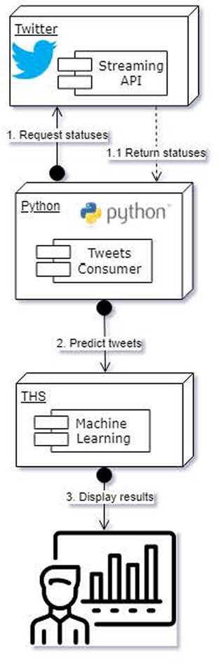
Tweet Prediction Pipeline

IV. Training and Classification of Tweets

In this section, we provide further details on how we train classifiers to determine if a tweet is related to a medical condition.

A. Preprocessing tweets

We pre-process our data set by eliminating all emojis, web links, hashtags, and twitter mentions that were embedded in each tweet. While developing our models and making initial training runs, we did not notice much difference between using word stemming or not. The same applies to removing stop words or not. Hence, we used neither stemming nor stop word elimination in the experiments shown in section V.

B. Mapping words to word embeddings

Once the tweets have been pre-processed, we need to convert from text to a tensor representation. One option is to create a dictionary of words, with each word w_i having a position i in the dictionary. Then, a tweet can be represented with a one-hot encoding vector representation. In this scheme, a vector v representing a tweet t will have position v[i] = 1, if word i is present in the tweet, or 0 otherwise. However, this approach has two main drawbacks. First, since the dictionary can have thousands of words, the vector v can be very long and mostly contain 0s. Secondly, with one-hot representation the order of words within the tweet is lost and can yield inaccurate results.

In THS, we use the well-known word embedding methodology [13], in which there is an embedding function that maps each word w_i in a tweet t into a vector v_i in an n-dimensional vector space Rⁿ. A Tweet t then becomes represented as a m × n matrix $\mathcal{M}$, where m is the longest tweet length and n is the dimension of the vector space. Conceptually, each row i in $\mathcal{M}$ is a vector v_i representing word w_i. Since not all tweets have the same length, padding with one or more instances of a zero vector is need to make all tweets in a batch have the same length.

In practice, the tweet t must first be mapped into a list of word indices L. Entry L[i] contains the position of word i in the dictionary used by the embedding. The embedding takes this index L[i] and maps it to a vector v_i

Word embeddings provide a better representation of the data, and it has been shown that related words in the target language tend to be mapped to close vectors in the vector space [13]. Moreover, word embedding are amicable for processing by deep learning models based on recurrent neural networks (RNN) and convolutions neural networks (CNN).

C. Processing with Recurrent Layers

THS uses recurrent neural networks (RNN) as the main ML building block for classification operations. RNN are designed for problems related with sequential data such as natural language processing. We use Long short-term memory (LSTM), and Gated recurrent units (GRU) as these are the best performing networks to date.

Figure 5 show the general architecture of the RNN that we used. This network is a classic encoder-decoder network. On the left, we have the batches of tweets to be fed into the network. The first stage of the network is the embedding layer, which takes care of mapping each tweet t into a embedding $\mathcal{M}$. The embedding is then feed into the first recurrent layer, which can be configured to use LSTM or GRU. This layer works as an encoder unit. Unless otherwise specified, the LSTM and GRU layers used 72 units. This number comes from the maximum tweet length that our testing data sets had. The next layer is a dropout layer used to prevent overfitting on the first recurrent layer. An optional attention layer [14] is added next. This layer is used to help focus the RNN into sections of the tweets that might be more important than others. If the attention layer is used, then the RNN must output all intermediate sequence outputs.

Figure 5:

General RNN Architecture

The next layer in the network is another recurrent layer that acts as the decoder component. Its output is passed to another dropout layer, and then to a dense layer containing 64 hidden units. The output of this layer is passed to a final softmax layer with 3 hidden unit which outputs a vector with the probabilities for each of the three classes.

In our current implementation, we provide the following concrete models based on this RRN architecture:

• 2 LSTM Tanh Attention - 2 LSTM with Tanh activation, and attention

• 2 LSTM elu Attention - 2 LSTM with lu activation, and attention

• GRU GRU No Attention - 2 GRU units without attention

• GRU GRU Attention - 2 GRU units with attention

• LSTM GRU No Attention - LSTM followed by GRU without attention

• GRU LSTM No Attention - GRU followed by LSTM without attention

• LSTM GRU Attention - LSTM followed by GRU with attention

• GRU LSTM Attention - GRU followed by LSTM with attention

• 2 LSTM Tanh Attention 100 Units - 2 LSTM with 100 hidden units, Tanh activation, and attention

• 2 LSTM elu Attention 100 Units - 2 LSTM with 100 hidden units, ell activation, and attention

In the future, we shall expand THS to incorporate convolutional neural networks (CNN) as part of the set of models than can be used for classification purposes.

V. Evaluation

A. Data Sets

We collected a total of 56,013 tweets from the Twitter API between March 7th and 28th, 2018. The tweets contain at least one of the following medical keywords:

• Zika

• Flu

• Ebola

• Measles

• Diarrhea

We then extracted a random sample of 12,500 tweets for labelling purposes. The labeling process was done in twenty nine days (29) by four members of our team. As mentioned before, we used three class labels: a) 0 - tweet is not about diseases, b) 1 - tweet is related with diseases, and c) 2 - tweet is ambiguous. Table I shows a distribution of the label classes in our labelled data set. As we can see, the data is unbalanced. In section V-C we describe how we handled this situation.

B. Experimental Setup

We implemented THS using open source software: Spark, Hive, HDFS, Kafka, TensorFlow, and Keras. Table II depicts the specific version of the components.

We ran our training procedures on nodes of the NSF-funded Chameleon Testbed. The nodes used are Dell PowerEdge R730, with 2x Intel(R) Xeon(R) CPU E5–2670 v3 @ 2.30GHz, 128 GB of RAM, 1 NVIDIA Tesla P100 GPU, 232 GB Seagate SATA HD. The machines ran the Ubuntu 16.04 LTS OS on bare metal. We trained several models independently of different nodes with the same configuration. The other THS components ran on a cluster at the University of Puerto Rico, Mayaguez, consisting of 12 (twelve) Dell Power Edge R420 with Intel Xeon Quad Core CPU, 8 GB RAM, 1TB disk, and 1Gbps NiC. These nodes ran Ubuntu 14.05 LTS on bare metal.

C. Experimental Methods

To train our ML models, our training program read the entire data set into memory, randomly shuffled all tweets, and then randomly assigned each tweet into one of three sub-sets:

• Training set (60% of the data) - this data set was used to train each ML model.

• Development set (20% of the data) - this second data set was used to fit the hyper parameters in the model, and determine which where the best performing candidates.

• Test set (20% of the data) - this third data set was used to give an unbiased evaluation of the candidate models and pick the best performing one for the metric at hand.

We used the shuffle functionality in Keras to shuffle training and development data. We also used the scikit-learn built-in support for K-fold cross-validation, but found very little difference between the two approaches.

Since most ML models assume a uniform distribution of examples among the classes present in the data, we had to find a way to adjust our models for the fact that we were working with imbalanced classes. We decided on two approaches to handle this situation. First, we ditched accuracy as our performance metric and instead use precision, recall, and F1 score. Notice that with an imbalanced class, a classifier might simply always predict in favor of the majority class. Hence, accuracy might not be the most adequate metric. For the validation and test phases, we compute a confusion matrix to collect the performance metrics on each model.

The second decision was to used a penalized model approach. Under this scheme, an additional penalty is added to the cost function whenever a model misclassifies, during training, an example that belongs to one of the minority classes. We used the built-in functionality in scikit-learn to estimate class weights penalties for imbalanced datasets. Table III shows the class weights used for our experiments. As we can see form the figure, the penalty for misclassifying an example in the minority class is substantially larger than that for the majority class. We considered using other approaches for class imbalance, such as oversampling the minority classes, or creating synthetic examples. However, we felt that weight penalization provided the most natural and straightforward method. In the future, we will experiment with those other approaches for imbalances data sets.

The hyper parameters for our models were selected using a custom-built grid search python code. The hyper parameters that we searched where: learning rate, number of epochs, batch size, percentage of dropout regularization, number of units for the dense layers, and optimization algorithm. In all the cases, RMSProp was the best algorithm for training out models. Thus, in the results that we show below all the models were trained using RMSProp.

In our experiments, we used the Glove embedding [15] with 50-dimensions for the embedding layer. Also, the longest tweet had 72 words, hence all tweets are padded to this length.

In the next section, we show the performance of the classifiers on the test sets.

D. Results

1). Precision:

The precision metric measures the exactness of a classifier, in terms of how many examples of a class i it correctly classifies. Given a class i, the precision on class i, P_i is defined as:

$$P_i=\frac{T{P}_i}{T{P}_i+F{P}_i}$$

Here T P_i is the number of correctly classified examples (true positive examples), while F P_i is the number of examples incorrectly labeled as belonging to class i (false positives). Thus, the precision on class i is a ratio between the number of correctly classified examples T P_i, and the sum of T P_i and F P_i. The closer P_i is to 1, the more exact the classifier is on class i.

Table IV shows the results for the precision metrics for class 1. For the sake of clarity, we only present this class. In addition, it is the most relevant class for the purpose of using Twitter to detect conversations about diseases. We shall present the complete results in a forthcoming paper devoted exclusively to the ML components in THS. Notice that the best performing model has a precision of 96%. This model contains a GRU layer followed by an LSTM layer with attention. This model took 10 epochs to train, and a 32 units dense layer after the LSTM and before the softmax output. Also, notice that the best performing models contain either an attention layer or an LSTM layer

2). Recall:

The recall metric provides a measure of how complete is the classifier in correctly labeling the examples of a class i. Given a class i, the recall on class i, R_i is defined as:

$$R_i=\frac{T{P}_i}{T{P}_i+F{N}_i}$$

As before, T P_i is the number of true positive examples for class i, whereas F N_i is the number of examples from class i that were missed by the classifier (false negatives). Recall is a ratio between T P_i, and the sum of T P_i and F N_i. In other words, recall tells what percentage of the examples of class i the classifier correctly detects and labels.

Table V shows the results for the recall metric for class 1. Notice that in this case only one model breaks over 90% in recall. This model has two GRU layers without attention, and has 92% recall. If we look this model into the table for precision (table IV) we can see that the model with the best precision (GRU LSTM Attention) has a “middle-of-the-road” performance in terms of recall. Thus, user of THS will need to decide which metric to prioritize and choose the right model accordingly. We also think that there is a certain amount of overfitting in these models, and we plan to address this issue by labeling more tweets to reach a data set size of at least 25,000 labelled tweets.

3). F1 Score:

Whether precision or recall is the right metric is a matter of debate (often a bitter debate). For some applications, recall is more important. For example, consider a medical application where a classifier is used to aid in the diagnosis of cancer. In this scenario, recall is the best metric since the priority is not to misdiagnose (i.e., miss the cancer) a patient by telling that he/she is cancer free when in fact the person has cancer (false negative). A false positive, although worrisome, is acceptable since it is better to err on the side of caution. On the other hand, in a surveillance application, having too many false positives can result in the unnecessary activation of alarms and security personnel (i.e., many false alarms), hence precision might be a better metric.

The F1 score is a metric that seeks to balance precision and recall, proving a method to determine how balanced a classifier is. The F1 score for class i is defined as follow:

$$F{\text{1}}_i=2\frac{P_i{R}_i}{P_i+R_i}$$

Notice that a classifier that is balanced will have an F1 score close to 1 since both the numerator and denominator will trend to 1. In contrast, a classifier biased toward either precision or recall will have a numerator that trends towards 0.

Table VI shows the results for the F1 score on class 1. The best performing model has an LSTM layer followed by a GRU layer without attention. This model is not the best in terms of either recall or precision, but it its the most balanced one. Interestingly, the model with two GRU units and no attention has a score of 90.50 %, making it a good overall choice since it has the best recall (92.32%) and decent precision (88.74%). We claim this because in our view, getting a good recall (i.e., not missing tweets) is more important than precision for the problem of detecting conversations about diseases in Twitter.

VI. Related Works

Sentiment analysis and opinion mining [16], [17], [18], [19], [20], [21] is a popular technique to analyze social media, blogs, and news articles in search for keywords that denote positive or negative views against a particular product, person, or situation. Clues about health conditions affecting citizens of a region can be obtained from the public messages that these citizens post in social media apps such as Twitter. In fact, recent research work has focused on using Twitter as a tool to help uncover health trends [1], [2], [3], [4], [5], [6], [7], [8], [9], [10] by looking at keywords in the messages that mention specific health conditions. THS leverages on many of these techniques, while proving a turn-key solution to build applications without much boiler plate code, and accessing the live Twitter stream instead of using a curated collection. To the best of our knowledge no other system offers the capabilities that THS has.

VII. Conclusion

In this paper, we have presented the Twitter Health Surveillance (THS) application framework. THS is designed as an integrated platform to help health officials collect tweets, determine if they are related with a medical condition, extract metadata out of them, and create a warehouse that can be used to further analyze the data. THS is built atop open source tools and provides the following value added services: Data Acquisition, Tweet Classification, and Big Data Warehousing. In order to validate THS, we have created a collection of roughly twelve thousands labelled tweets. These tweets contain one or more target medical terms, and the labels indicate if the tweet is related or not to a medical condition. We used this collection to test various models based on LSTM and GRU recurrent neural networks. Our experiments show that we can classify tweets with 96% precision, 92% recall, and 91% F1 score. These results compare favorably with recent research on this area, and show the promise of our THS system.

Table I:

Distribution of tweets per class label.

Class Label	Tweet Count
0	3,850
1	7,917
2	733

Table II:

Version for software packages used in THS.

Software Package	Version
Spark	2.1
Hive	2.2
HDFS	2.7
Kafka	0.10.1
TensorFlow	1.10
Keras	2.1.6
scikit-learn	0.19.2

Table III:

Class weight penalties.

Class	Penalty Weight
0	1.08225108
1	0.52629363
2	5.684402

Table IV:

Precision results per ML model

Model	Presicion
2 LSTM Tanh Attention	0.910204082
2 LSTM elu Attention	0.923603193
GRU GRU No Attention	0.887412041
GRU GRU Attention	0.94934877
LSTM GRU No Attention	0.939040208
GRU LSTM No Attention	0.89198036
LSTM GRU Attention	0.883814103
GRU LSTM Attention	0.962479608
2 LSTM Tanh Attention 100 Units	0.95021645
2 LSTM elu Attention 100 Units	0.930857875

Table V:

Recall results per ML model

Model	Recall
2 LSTM Tanh Attention	0.809314034
2 LSTM elu Attention	0.852737571
GRU GRU No Attention	0.923222152
GRU GRU Attention	0.835116425
LSTM GRU No Attention	0.891755821
GRU LSTM No Attention	0.784140969
LSTM GRU Attention	0.861548143
GRU LSTM Attention	0.823788546
2 LSTM Tanh Attention 100 Units	0.877910636
2 LSTM elu Attention 100 Units	0.850220264

Table VI:

F1 results per ML model

Model	Fl
2 LSTM Tanh Attention	0.856799275
2 LSTM elu Attention	0.88675682
GRU GRU No Attention	0.904962976
GRU GRU Attention	0.888576312
LSTM GRU No Attention	0.914787402
GRU LSTM No Attention	0.834591544
LSTM GRU Attention	0.872539097
GRU LSTM Attention	0.887749888
2 LSTM Tanh Attention 100 Units	0.912633628
2 LSTM elu Attention 100 Units	0.888713651

References

- [1].Parker J, Wei Y, Yates A, Frieder O, and Goharian N, “A framework for detecting public health trends with twitter,” in Proceedings of the 2013 IEEE/ACM International Conference on Advances in Social Networks Analysis and Mining, ASONAM ‘13, (New York, NY, USA), pp. 556–563, ACM, 2013. [Google Scholar]
- [2].Aramaki E, Maskawa S, and Morita M, “Twitter catches the flu: Detecting influenza epidemics using twitter,” in Proceedings of the Conference on Empirical Methods in Natural Language Processing, EMNLP ‘11, (Stroudsburg, PA, USA), pp. 1568–1576, Association for Computational Linguistics, 2011. [Google Scholar]
- [3].Culotta A, “Towards detecting influenza epidemics by analyzing twitter messages,” in Proceedings of the First Workshop on Social Media Analytics, SOMA ‘10, (New York, NY, USA), pp. 115–122, ACM, 2010. [Google Scholar]
- [4].Diaz-Aviles E, Stewart A, Velasco E, Denecke K, and Nejdl W, “Towards personalized learning to rank for epidemic intelligence based on social media streams,” in Proceedings of the 21st International Conference Companion on World Wide Web, WWW ‘12 Companion, (New York, NY, USA), pp. 495–496, ACM, 2012. [Google Scholar]
- [5].Paul MJ and Dredze M, “Discovering health topics in social media using topic models,” PLoS ONE, vol. 9, p. e103408, 08 2014. [DOI] [PMC free article] [PubMed] [Google Scholar]
- [6].Ghenai A and Mejova Y, “Catching zika fever: Application of crowdsourcing and machine learning for tracking health misinformation on twitter,” in 2017 IEEE International Conference on Healthcare Informatics (ICHI), pp. 518–518, August 2017. [Google Scholar]
- [7].Bates M, “Tracking disease: Digital epidemiology offers new promise in predicting outbreaks,” IEEE Pulse, vol. 8, pp. 18–22, January 2017. [DOI] [PubMed] [Google Scholar]
- [8].Ji X, Chun SA, and Geller J, “Monitoring public health concerns using twitter sentiment classifications,” in 2013 IEEE International Conference on Healthcare Informatics, pp. 335–344, September 2013. [Google Scholar]
- [9].Culotta A, “Towards detecting influenza epidemics by analyzing twitter messages,” in Proceedings of the First Workshop on Social Media Analytics, SOMA ‘10, (New York, NY, USA), pp. 115–122, ACM, 2010. [Google Scholar]
- [10].Jiang K, Feng S, Song Q, Calix RA, Gupta M, and Bernard GR, “Identifying tweets of personal health experience through word embedding and lstm neural network,” BMC Bioinformatics, vol. 19, p. 210, June 2018. [DOI] [PMC free article] [PubMed] [Google Scholar]
- [11].Batista GEAPA, Prati RC, and Monard MC, “A study of the behavior of several methods for balancing machine learning training data,” SIGKDD Explor. Newsl, vol. 6, pp. 20–29, June 2004. [Google Scholar]
- [12].He H and Garcia EA, “Learning from imbalanced data,” IEEE Transactions on Knowledge and Data Engineering, vol. 21, pp. 1263–1284, September 2009. [Google Scholar]
- [13].Mikolov T, Chen K, Corrado G, and Dean J, “Efficient estimation of word representations in vector space,” CoRR, vol. abs/1301.3781, 2013. [Google Scholar]
- [14].Bahdanau D, Cho K, and Bengio Y, “Neural machine translation by jointly learning to align and translate,” CoRR, vol. abs/1409.0473, 2014. [Google Scholar]
- [15].Pennington J, Socher R, and Manning CD, “Glove: Global vectors for word representation,” in In EMNLP, 2014. [Google Scholar]
- [16].Choi Y, Kim Y, and Myaeng S-H, “Domain-specific sentiment analysis using contextual feature generation,” in Proceedings of the 1st International CIKM Workshop on Topic-sentiment Analysis for Mass Opinion, TSA ‘09, (New York, NY, USA), pp. 37–44, ACM, 2009. [Google Scholar]
- [17].Kim S-M and Hovy E, “Determining the sentiment of opinions,” in Proceedings of the 20th International Conference on Computational Linguistics, COLING ‘04, (Stroudsburg, PA, USA), Association for Computational Linguistics, 2004. [Google Scholar]
- [18].Wang H, Can D, Kazemzadeh A, Bar F, and Narayanan S, “A system for real-time twitter sentiment analysis of 2012 u.s. presidential election cycle,” in Proceedings of the ACL 2012 System Demonstrations, ACL ‘12, (Stroudsburg, PA, USA), pp. 115–120, Association for Computational Linguistics, 2012. [Google Scholar]
- [19].Fan W and Gordon MD, “The power of social media analytics,” Commun. ACM, vol. 57, pp. 74–81, June 2014. [Google Scholar]
- [20].Arias M, Arratia A, and Xuriguera R, “Forecasting with twitter data,” ACM Trans. Intell. Syst. Technol, vol. 5, pp. 8: 1,–8: 24, Jan. 2014. [Google Scholar]
- [21].Tsytsarau M, Amer-Yahia S, and Palpanas T, “Efficient sentiment correlation for large-scale demographics,” in Proceedings of the 2013 ACM SIGMOD International Conference on Management of Data, SIGMOD ‘13, (New York, NY, USA), pp. 253–264, ACM, 2013. [Google Scholar]