The normal range: it is not normal and it is not a range

Abstract

The NHS ‘Choose Wisely’ campaign places greater emphasis on the clinician-patient dialogue. Patients are often in receipt of their laboratory data and want to know whether they are normal. But what is meant by normal? Comparator data, to a measured value, are colloquially known as the ‘normal range’. It is often assumed that a result outside this limit signals disease and a result within health. However, this range is correctly termed the ‘reference interval’. The clinical risk from a measured value is continuous, not binary. The reference interval provides a point of reference against which to interpret an individual’s results—rather than defining normality itself. This article discusses the theory of normality—and describes that it is relative and situational. The concept of normality being not an absolute state influenced the development of the reference interval. We conclude with suggestions to optimise the use and interpretation of the reference interval, thereby facilitating greater patient understanding.

The ‘Choose Wisely’ campaign was introduced by the Academy of Medical Royal Colleges in 2016 with a view to encouraging a dialogue between clinician and patient regarding the practice of evidence-based treatment regimens.¹ Clinicians have access to a vast array of investigations and interpretation of the results of these tests is central to our role. A fundamental question that the patient wants answered is ‘are my tests normal?’

But what is meant by ‘normal’?

With every test result, the clinical laboratory will provide comparator value(s) to help the clinician place the result in context. The comparator values are often referred to as the normal range. A frequent occurrence is for the results within this interval to be colour coded, for instance black if the result is within the range and red when outside of it. This reinforces the concept of a result having a binary quality: normal or abnormal.

If we say that a blood result is normal, a number of inferences of dissimilar nature could be put on this. The difficulty was neatly captured by the philosopher Edmond Murphy in 1960s (table 1).² In the clinical setting, our experience is that the term is frequently used to imply that the patient has no physiological derangement and/or that the distribution follows a Gaussian distribution.

Table 1.

Interpretations of ‘normal’ (modified from Murphy, 1966²)

	Conceptions of normal	Suggested alternatives
1	Determined statistically	Gaussian
2	Most representative of its class	Average, median, modal
3	Most commonly encountered	Habitual
4	Wild-type: most suited to survival & reproduction	Fittest
5	Harmless ‘carrying no penalty’	Innocuous/harmless
6	Most often aspired to	Conventional
7	The most perfect of its class	Ideal

If it is assumed that a ‘normal’ result has no pathophysiological derangement, the corollary would be that a result outside this limit would signal a disease state. This seems an arbitrary dichotomous interpretation. As the American psychiatrist, Theodore Rubin, put it ‘health may be considered a relative and not an absolute state’. Health may be conceived differently in different countries, or in the same country at different times, or even in the same individual at different ages.

How did the ‘normal range’ develop? First, some semantics; the reference limit is the upper and lower extreme of the reference interval, whereas the reference range refers to the difference between two values. If, for instance, we take the upper and lower reference limits for sodium as 135 and 145 mmol/L, respectively, the range is 10 mmol/L while the interval is 135–145 mmol/L. An observed value is a value of a particular type obtained by measurement (blood testing), produced to make a medical decision: this may then be compared with a reference limit or reference interval.

Until the 1960s, laboratories often worked in isolation and developed their own comparator values to define normal limits. It became apparent that multiple ‘normal ranges’ were required for different patient populations and for individual laboratories, to account for methodological variation. The clinical practice at the time was to compare a patient’s results with an ill-defined or at least inconsistently defined, range of values—called the ‘normal range’). This was derived from a population of supposedly ‘normal’ (meaning healthy) individuals. The concept of the reference interval was then introduced by Grasbeck and Saris in 1969³ as it was felt that the concept of a normal range, as then conceived, was flawed. The reference interval was designed to describe fluctuations of blood analyte concentrations in well-characterised groups of individuals in order to replace the more ambiguous concept of normal values. The intention was to have a point of reference against which to interpret an individual’s results—rather than defining normality itself. Normality is relative and situational. The population reference interval may not account for factors such as age, ethnicity or gender unless they have a major impact. Therefore, the reference interval is an approximation of what can be expected in the population. This difficulty has been recognised in critical care medicine leading to calls for the development of a new normative data base for the critically ill.⁴

Often what underpins both these methods is the assumption that using a Gaussian distribution, to identify the middle 95% of individuals, will identify healthy individuals. There are three criticisms of the use and terminology applied here; First, values may not fall into a bell-shaped distribution but can be skewed. Fasting triglyceride is a good example of this. The most common triglyceride value (the mode) is not found at the midpoint of the population density curve but to one side—the distribution is skewed to the right (figure 1).

Figure 1.

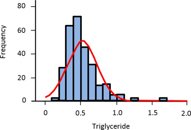
Fasting triglyceride as an example of a skewed (non-Gaussian) distribution.

Second, no underlying theory assumes that the central 95% is physiologically normal. The 95% interval is based on pragmatism—two SD from the mean was considered suitably distant from the mean and was taken from Fisher’s development of the hypothesis-testing technique of Neyman and Pearson.⁵ However, there is no reason why the central 90% could not be used—although such an approach would increase false positives or the central 99%—although this would increase the rate of false negatives.

Third, the bell-shaped distribution that we term the ‘normal distribution’ is something of a misnomer. It was commonly referred to as ‘Gaussian’ until another mathematician, Karl Pearson, adopted the term ‘normal distribution’, referring to the fact that the distribution pattern was ubiquitous in life. The term was not introduced for its propensity to identify ‘normal’ individuals.⁶ For instance, a blood urea value at the upper end of the reference interval may represent significant renal impairment in an individual who has liver dysfunction and cannot adequately synthesise urea.

Just as a result within the reference interval may be ‘abnormal’, so might a result outside the interval be ‘normal’ (seen in the presence of health). For instance, mild hyponatraemia in the elderly may not necessarily represent disease. Physiological changes associated with ageing can include elevated antidiuretic hormone and atrial natriuretic hormone levels as well as an increased responsiveness to osmotic stimulation.⁷ It is extremely unusual in nature for the two distributions (of health and disease) to be separate and discrete (figure 2). Disease and health are not dichotomous but are dynamic, inter-related and the variables to define them usually overlap (figure 3).

Figure 2.

Two Gaussian distributions with no overlap.

Figure 3.

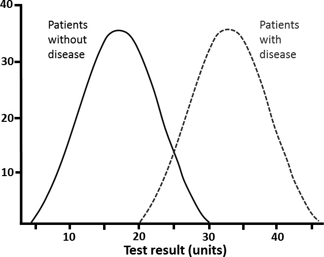
Overlapping Gaussian distributions.

Thus, it can be seen that a patient may be classed as healthy at an individual level but diseased at a population level and vice versa (figures 3 and 4).

Figure 4.

Detection of an outlier.

The laboratory report seldom features one value in isolation. Rather, a whole panel of tests are requested, analysed and reported, such as U&Es, LFTs, bone profile; cumulatively, these are sometimes referred to as a comprehensive metabolic panel. What are the chances that out of a panel of tests, one will be abnormal? We can use the binomial distribution to test this. In statistics, the binomial distribution has only two outcomes: ‘success or failure’, ‘positive or negative’, ‘yes or no’. The binomial equation to determine the probability (p) of a single ‘success’ when performing a sequence of n independent tests is:

$${\displaystyle (1-p{)}^{\mathrm{n}-1}}$$

The chance of a positive blood test result (‘success’) is 0.05 (because 5% of population values lie outside the normal distribution and, as described above, in this instance are considered as abnormal). Therefore, the probability that one result is abnormal in a panel of 20 tests is:

$${\displaystyle (1-0.05{)}^{20-1}={0.95}^{19}=0.38}$$

There is therefore a 38% chance that 1 of the 20 of the tests will be abnormal. This value is indicative only, as it assumes independence of the analytes being tested, whereas often they are related, for example, alkaline phosphatase may change in tandem with gamma-glutamyl transferase.

How can the reference limit support a decision? How can it discriminate?

We have described that the clinical risk from an observed value is continuous and so we must take care that the reference limit is not confused with a decision limit. This is a different way of conveying information; an observed value is still presented but there is less ambiguity in how the clinician should respond at or beyond the decision limit. A decision limit is based on the sensitivity and specificity of a test at various threshold test settings. A good example of this is the glycated haemoglobin (HbA_1c)—a value of 42 mmol/mol is considered ‘normal’ and 48 mmol/mol is, with specific preanalytic criteria met, consistent with a diagnosis of diabetes mellitus. If, instead of a decision limit to diagnose diabetes, a reference interval was used (where only the outlying 5% of the population are considered ‘abnormal’), a large number of individuals who currently have the diagnosis of diabetes would be reclassified as ‘normal’. This is because, using a decision limit, the prevalence of diabetes in England is estimated at 9% of the adult population,⁸ whereas it would drop to 2.5% if HbA_1c>2 SD from the mean (ie, the tail of a Gaussian distribution) were used instead to determine diabetes.

The differences between reference intervals and decision limits are summarised in table 2 (modified from Ceriotti et al ⁹). Decision limits are appearing more frequently in laboratory reports. They have the advantage of making decisions more reproducible but reproducibility is not always helpful, especially if the benefits of a decision limit are applied to the wrong population. The ubiquity of decision limits may also entrench the idea of applying categorical outcomes to continuous data.

Table 2.

Features of a decision limit and a reference interval (modified from Ceriotti and Henny, 2008⁹)

	Reference intervals	Decision limits
Definition	The interval between, and including, two reference limits, which are values derived from the distribution of the results obtained from a sample of the reference population.	The best dividing lines between the diseased and the not diseased or between ‘those who need not be investigated further’ and ‘those who do’.
Conditions influencing them	Population Age group Gender	Clinical question Patient category
Information gathered	Whether or not the patient is part of the reference population	Whether or not the patient is eligible for a certain procedure (‘treatment’)
Statistics	95% central range of the distribution curve	None (consensus values) ROC curves Predictive values
Data number	Two (lower and upper limits)	One, without any CI There can sometimes be >1, but according to the likelihood of various clinical situations or different clinical questions

ROC, receiver operating characteristic.

What could be done?

Language is important, as we see from table 1, normal means different things to different people, and to the same person in different circumstances. The phrase ‘normal range’ is unhelpful and inaccurate.

1. Question why the information is being gathered. Is it for benchmarking for the future; screening; completing a panel or performing a diagnostic investigation?

2. Will the investigation change the odds of something? Consider limiting indiscriminate testing.

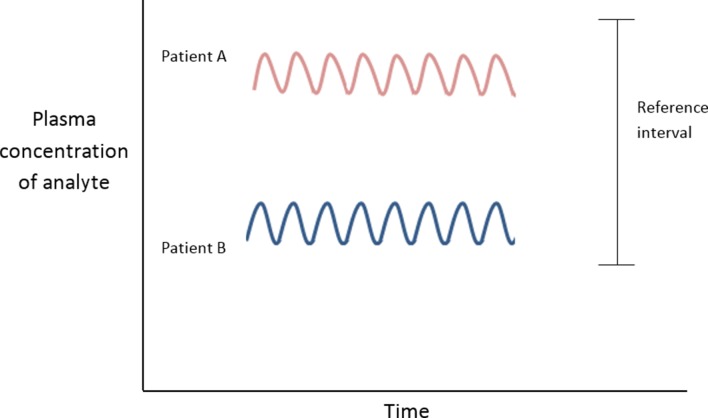
3. Relate the observed value to preceding values whenever possible. The intraindividual variation in laboratory values is usually much smaller than the interindividual variability (ie, the variation in the population; figure 5). Variation in the concentration of an analyte, if significantly outside of a patient’s usual values (but still within the reference interval), could be a sign of early or latent disease.¹⁰ Thus, a haemoglobin of 130 g/L in a male, though within the reference interval (130–180 g/L), might represent a fall from (unmeasured) 170 g/L. The result must be interpreted in the light of the clinical history.

Figure 5.

Interindividual variation greater than intraindividual variation.

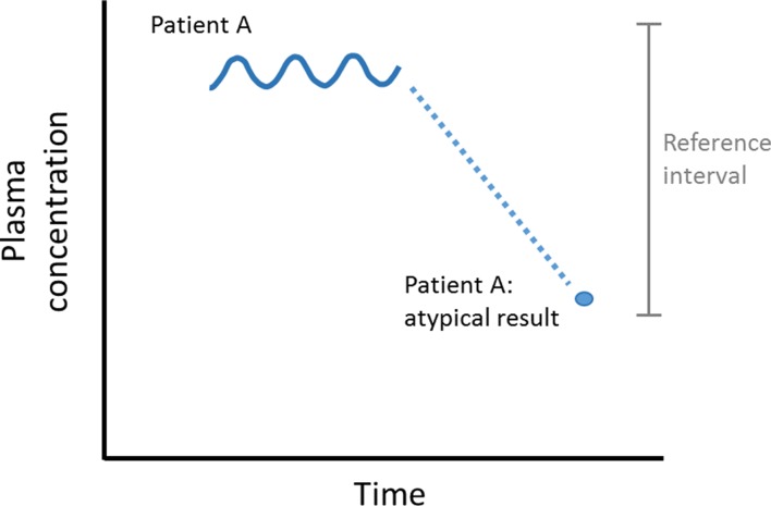
The graphical representation of preceding data (if available) can be extremely effective in identifying trends (figure 4). The atypical result for Patient A may be due to:

• Preanalytical error (how the sample was taken or transported to the laboratory).¹¹

• Analytical error (how the sample was processed in the laboratory).

• Intraindividual fluctuations of the variable measured (unlikely given the pattern of variation up to that point).

• A real pathology. Attempts have been made to capture this from a ‘critical difference calculation’. The critical difference is defined as ‘the smallest difference between sequential laboratory results in a patient which is likely to indicate a true change in the patient’ and the calculation requires specifics of the laboratory (analytical) variation as well as within-subject biological variation.¹²

In this situation, assuming that no pretest probability had been estimated (ie, that the sample was not specifically requested to test a theory), the sample may be: (1) supplemented by historic data and further findings—as with the example above (enhancement or lowering of probability that they form a component of disease).

(2) Repeated (reduces the chances being secondary to a preanalytic or analytic error or to intraindividual fluctuations). Repetition, if chosen, should be made at intervals appropriate to the expected rate of development of possible disease. The observed value on repetition may well have shifted closer to the centre of the reference interval—a phenomenon known as ‘regression to the mean’.

Regression to the mean

This is a statistical tendency where unusually large or small measurements tend to be followed by measurements that are closer to the mean¹³ (figure 6). The term was introduced by Francis Galton in the late 19th century as a consequence of his investigations of the relationship between the heights of parents and their children. The heights of children of very tall parents tended to be shorter (and vice versa) so that over time it ‘regressed’ (or ‘reverted’) to the population mean. In medicine, this phenomenon can sometimes suggest an efficacy of a treatment—that may in fact be having no effect at all.

Figure 6.

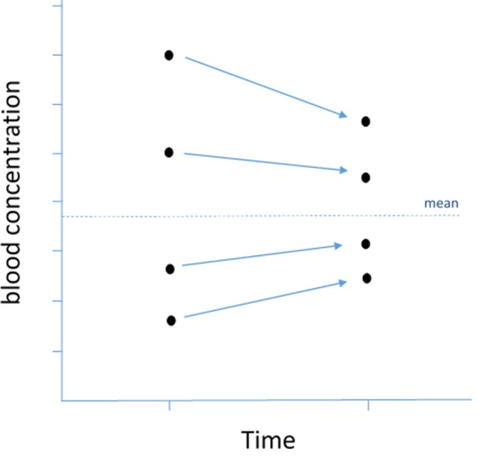
Regression to the mean. On repetition, values furthest from the mean tend to have greater change than values starting close to the mean.

Conclusion

The reference interval is an extremely useful means of contextualising a patient’s result but it is wrong to automatically assume ‘normality’ of a result within that interval, just as it is wrong to assume abnormality outside of the interval. Normality is relative and situational. With understanding of the nature of the reference interval, logical decisions can be made that will improve the effectiveness of the clinical consultation.

Main messages.

• Health is a relative and not an absolute state.

• The reference interval acts as a comparator for the patient’s blood result. It is not the arbiter of whether disease is present or not.

• Natural fluctuations in a blood result can occur.

• Comparison of a result against the reference interval should be informed by the clinical suspicion made beforehand.

References

- 1. Wise J. Choosing Wisely: how the UK intends to reduce harmful medical overuse. BMJ 2017;356:j370 10.1136/bmj.j370 [DOI] [PubMed] [Google Scholar]
- 2. Murphy EA. A scientific viewpoint on normalcy. Perspect Biol Med 1966;9:333–48. 10.1353/pbm.1966.0011 [DOI] [PubMed] [Google Scholar]
- 3. Gräsbeck R. The evolution of the reference value concept. Clin Chem Lab Med 2004;42:692–7. 10.1515/CCLM.2004.118 [DOI] [PubMed] [Google Scholar]
- 4. Kilickaya O, Schmickl C, Ahmed A, et al. . Customized reference ranges for laboratory values decrease false positive alerts in intensive care unit patients. PLoS One 2014;9:e107930 10.1371/journal.pone.0107930 [DOI] [PMC free article] [PubMed] [Google Scholar]
- 5. Fisher R. Statistical methods for research workers. 5th edn Edinburgh, UK: Oliver & Boyd, 1934. [Google Scholar]
- 6. Wilcox RR. Understanding and applying basic statistical methods using R. Wiley, 2016. [Google Scholar]
- 7. Cowen LE, Hodak SP, Verbalis JG. Age-associated abnormalities of water homeostasis. Endocrinol Metab Clin North Am 2013;42:349–70. 10.1016/j.ecl.2013.02.005 [DOI] [PMC free article] [PubMed] [Google Scholar]
- 8. Diabetes prevalence estimates for local populations. Secondary Diabetes prevalence estimates for local populations. 2015. Available from: https://www.gov.uk/government/publications/diabetes-prevalence-estimates-for-local-populations
- 9. Ceriotti F, Henny J. "Are my Laboratory Results Normal?" Considerations to be Made Concerning Reference Intervals and Decision Limits. EJIFCC 2008;19:106–14. [PMC free article] [PubMed] [Google Scholar]
- 10. Harris EK. Effects of intra- and interindividual variation on the appropriate use of normal ranges. Clin Chem 1974;20:1535–42. [PubMed] [Google Scholar]
- 11. Whyte MB, Vincent RP. How the routine reporting of laboratory measurement uncertainty might affect clinical decision making in acute and emergency medicine. Emerg Med J 2016;33:278–9. 10.1136/emermed-2015-205438 [DOI] [PubMed] [Google Scholar]
- 12. Jones GR. Critical difference calculations revised: inclusion of variation in standard deviation with analyte concentration. Ann Clin Biochem 2009;46(Pt 6):517–9. 10.1258/acb.2009.009083 [DOI] [PubMed] [Google Scholar]
- 13. Bland JM, Altman DG. Regression towards the mean. BMJ 1994;308:1499. [DOI] [PMC free article] [PubMed] [Google Scholar]