Assessment of Convolutional Neural Networks for Automated Classification of Chest Radiographs

Abstract

Purpose

To assess the ability of convolutional neural networks (CNNs) to enable high-performance automated binary classification of chest radiographs.

Materials and Methods

In a retrospective study, 216 431 frontal chest radiographs obtained between 1998 and 2012 were procured, along with associated text reports and a prospective label from the attending radiologist. This data set was used to train CNNs to classify chest radiographs as normal or abnormal before evaluation on a held-out set of 533 images hand-labeled by expert radiologists. The effects of development set size, training set size, initialization strategy, and network architecture on end performance were assessed by using standard binary classification metrics; detailed error analysis, including visualization of CNN activations, was also performed.

Results

Average area under the receiver operating characteristic curve (AUC) was 0.96 for a CNN trained with 200 000 images. This AUC value was greater than that observed when the same model was trained with 2000 images (AUC = 0.84, P < .005) but was not significantly different from that observed when the model was trained with 20 000 images (AUC = 0.95, P > .05). Averaging the CNN output score with the binary prospective label yielded the best-performing classifier, with an AUC of 0.98 (P < .005). Analysis of specific radiographs revealed that the model was heavily influenced by clinically relevant spatial regions but did not reliably generalize beyond thoracic disease.

Conclusion

CNNs trained with a modestly sized collection of prospectively labeled chest radiographs achieved high diagnostic performance in the classification of chest radiographs as normal or abnormal; this function may be useful for automated prioritization of abnormal chest radiographs.

© RSNA, 2018

Online supplemental material is available for this article.

See also the editorial by van Ginneken in this issue.

Summary

Convolutional neural networks trained using 20 000 labeled chest radiographs show promise for automated classification of chest radiographs as normal or abnormal, potentially enabling triage of studies in clinical practice.

Implications for Patient Care

• ■ Convolutional neural networks (CNNs) yield high performance (area under the receiver operating characteristic curve = 0.96) in the automated classification of chest radiographs as normal or abnormal.

• ■ An increase in training set size beyond 20 000 prospectively labeled chest radiographs, a modest data set size accessible to many institutions, yields only marginal benefit.

• ■ A combination of clinician assessment with CNNs output yields the best observed classifier.

Introduction

Chest radiography represents the initial imaging test for important thoracic abnormalities ranging from pneumonia to lung cancer. Unfortunately, as the ratio of image volume to qualified radiologists has continued to increase, interpretation delays and backlogs have demonstrably reduced the quality of care in large health organizations, such as the U.K. National Health Service (1) and the U.S. Department of Veterans Affairs (2). The situation is even worse in resource-poor areas, where radiology services are extremely scarce (3,4). In this light, automated image analysis represents an appealing mechanism to improve throughput while maintaining, and potentially improving, quality of care.

The remarkable success of machine learning techniques such as convolutional neural networks (CNNs) for image classification tasks makes these algorithms a natural choice for automated radiograph analysis (5,6), and they have already performed well for tasks such as skeletal bone age assessment (7–9), lung nodule classification (10), tuberculosis detection (11), high-throughput image retrieval (12,13), and evaluation of endotracheal tube positioning (14). However, a major challenge when applying such techniques to chest radiography at scale has been the limited availability of the large labeled data sets generally required to achieve high levels of performance (6). In response, the U.S. National Institutes of Health released a public chest radiograph database containing 112 120 frontal view images with noisy multiclass labels extracted from associated text reports (15). This study also showed the challenges of achieving reliable multiclass thoracic diagnosis prediction with chest radiographs (15), potentially limiting the clinical utility of resultant classifiers. Further, this method of disease-specific computer-assisted diagnosis may not ultimately be beneficial to the interpreting clinician (16).

In this context, we have curated a large clinician-labeled data set from our institution to assess the application of CNNs to automated classification of chest radiographs as normal or abnormal. Our hypotheses are (a) that simplifying the automated analysis problem to a binary triage classification task will lead to useful performance levels on a clinically relevant task using a prospectively labeled data set of a size accessible to many institutions and (b) that combining clinician judgment with CNN output will yield a triage classifier superior to either one alone. This work could be clinically important both by permitting radiologists to spend more time on abnormal studies and by demonstrating a simple mechanism to combine physician judgment with deep learning algorithms such as CNNs in a manner that can improve interpretation performance.

Materials and Methods

Data acquisition and processing in this retrospective study were approved by our institutional review board and were compliant with Health Insurance Portability and Accountability Act standards. Written informed consent was waived by the institutional review board because of the retrospective nature of this study, and all images were deidentified.

Data Set and Preprocessing Description

We procured 313 719 chest radiographs obtained at our institution between January 1, 1998, and December 31, 2012, along with the associated text report for each radiographic examination. All studies performed during this time were given one of six possible summary labels at the time of interpretation by an attending subspecialist radiologist, which were binned into “normal” or “abnormal” categories, as described in Appendix E1 (online).

After filtering these 313 719 radiographs for single-image anteroposterior or posteroanterior studies, 216 431 images remained, with a sex balance of 55% male (118 383 of 216 431) and a class balance of 79% abnormal (171 199 of 216 431). From this image collection, we randomly sampled 200 000 images to create a training set of 180 000 images and a development set of 20 000 images. Randomly selected subsamples of 1% and 10% size were created from training and development sets to assess the effect of data set size on end performance.

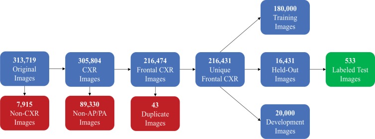
For final model evaluation, a balanced set of 1000 images (500 normal, 500 abnormal) from the 16 431 remaining images was labeled independently by two general radiologists with 20 (D.L.R.) and 5 (M.P.L.) years of experience. Each radiologist was originally supplied with the same set of images (with no accompanying prospective labels or reports). The normal and abnormal labels created by these two radiologists were then provided to a third party (J.A.D.), who identified radiographs with conflicting labels. Disagreements between the two raters were directly adjudicated by consensus, where prospective labels, text reports, and each radiologist’s first-round label were withheld during adjudication. Once these 1000 images were fully labeled, images with true-negative findings (ie, normal images) were removed, such that the class balance of the test set mirrored that of the training set. This process, summarized in Figure 1, yielded a set of 533 images that were ultimately used for evaluation.

Figure 1:

Flowchart of radiographs used in this study. AP = anteroposterior, CXR = chest x-ray, PA = posteroanterior.

All images underwent histogram equalization (scikit-image, version 0.14) for contrast enhancement (17), downsampling to a standard 224 × 224 input resolution to enable use of standard CNN architectures with pretrained weights (torchsample, version 0.1.3), and per-sample mean-standard deviation normalization (torchsample, version 0.1.3). Because of the large size of the base data set, no data augmentations were applied in our study.

Additional details on data set selection, labeling, and preprocessing can be found in Appendix E1 (online).

Model Architecture and Implementation

We trained several CNN models by using architectures that are well known in the literature, such as AlexNet (18), ResNet (19), and DenseNet (20), with the goal being to show the type of performance that can be achieved by using the current standard of off-the-shelf CNN-based image analysis algorithms, open-source software, and common hardware (eg, one GPU [graphics processing unit]). The standard CNN implementations used in this work are sourced from the torchvision (version 0.2.0) package contained within the PyTorch software framework (21). Weights for each architecture pretrained with the ImageNet database (6) can be found within the public repositories for these packages. In our implementation, the final linear layer of each network is replaced with one that reduces final output to one value that is operated on by a sigmoid nonlinearity. Exact details and parameters of the CNN training procedure (optimizer, batch sizes, preprocessing, etc) are provided in Appendix E1 (online).

When evaluating the use of deep learning techniques like CNNs that learn their own feature sets from data for a given image analysis task, comparison with machine learning methods based on predefined feature sets represents a natural baseline. Further, such methods can have utility in certain contexts because they rely on features that can be precomputed and are amenable to robust error analysis techniques. Thus, in this work, we also report results for the automated binary triage task obtained by using a kernelized support vector machine with bag-of-visual-words features, as described by Vedaldi and Zisserman (22) and implemented in the open-source VLFeat (version 0.9.18) library (23). All model training procedures, which are described in detail in Appendix E1 (online), leverage the analogous VLFeat implementations described by Vedaldi and Fulkerson (23) and accessed through the Matlab (version R2011; MathWorks, Natick, Mass) interface. Note that unlike the CNN models, which require high-performance GPU hardware, the kernelized support vector machine and bag-of-visual-words features models are trained in a comparable amount of time by using a modest number of CPU (central processing unit) cores.

Statistical Analysis

Performance was assessed by using the area under the receiver operating characteristic curve (AUC) and precision, recall, and F1 scores (these metrics are defined in detail in Appendix E1 [online]). These measurements were computed by using the scikit-learn (version 0.19) Python library and were reported for the test set in each model. Interrater agreement was assessed with the Cohen κ statistic and was also computed by using scikit-learn software. The DeLong nonparametric statistical test (24) implemented in the Daim (version 1.1.0) R library was used to assess statistical differences among AUC values, wherein P values less than .05 were considered to indicate a significant difference. The method described by Hanley and McNeil (25) was used to compute 95% confidence intervals for AUC values.

To enable accessible analysis of CNN model results, we created class activation maps (CAMs) that show the areas of a given image that are most responsible for its CNN classification (26). The CAMs we used were slightly different from those used by Zhou et al (26) because of the sigmoid nonlinearity on the final layer; however, they convey similar information about the contribution of a given region to the overall classification.

Results

Our first set of experiments was performed to investigate the effect of training set size, development set size, and initialization strategy (random vs pretrained with the ImageNet database) on end performance by using a relatively compute-efficient 18-layer residual network (ResNet-18) architecture (19). Five-fold cross-validated binary classification performance for each class is reported for all experiments in Table 1. Values other than AUC were computed by using an untuned threshold value of 0.5 on the neural network sigmoid output (a number between 0 and 1). In practice, this threshold could be tuned on the development set to optimize a chosen performance metric for the task at hand. Confidence intervals for the AUC values reflected that all models trained by using more than 2000 images yield AUC values greater than those trained by using 2000 images (P < .005). AUC values attained with models trained by using 200 000 or 20 000 images were not significantly different (P > .05). Additionally, outside of the case with 20 000 training points and 2000 development points (P < .05), variations in the size of the development set or the initialization strategy did not result in significantly different (P > .05) AUC values for any of the three training set sizes.

Table 1:

Performance Metrics for Different Set Sizes and Initializations

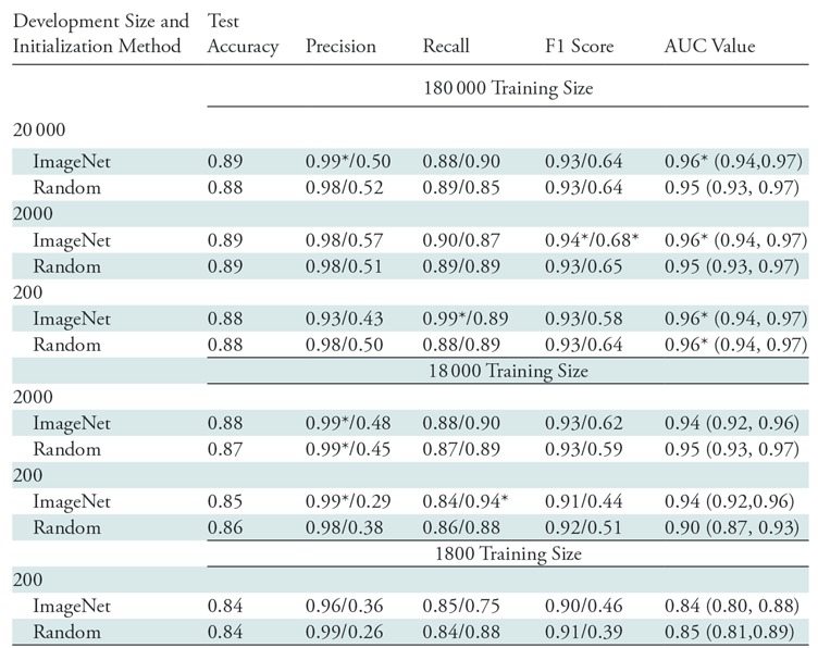
Note.—Comparison of performance metrics for different set sizes and initializations for ResNet-18. All metrics represent average values over five-fold cross-validation and are computed by using an untuned threshold value of 0.5. Data to the left of the virgule are for the abnormal class, and data to the right are for the normal class. Key descriptive statistics are total samples (n = 533), true abnormal (positive) findings (n = 423), and true normal (negative) findings (n = 110). Data in parentheses are 95% confidence intervals. AUC = area under the receiver operating characteristic curve.

*Data are best observed values.

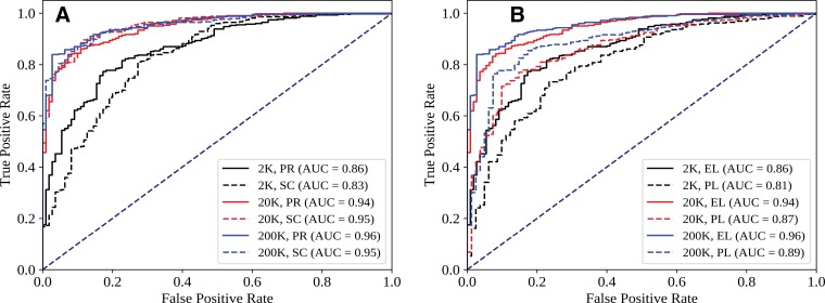
Figure 2 shows ROC curves for several pertinent conditions from Table 1. Figure 2, A, suggests that while performance across the ROC curve is minimally affected by initialization for larger data sets, initialization differences can noticeably affect tradeoffs between sensitivity and specificity in the high-specificity regimen. Figure 2, B, shows more favorable sensitivity and specificity tradeoffs throughout the ROC curve when CNN performance is evaluated with respect to the expert labels as opposed to the original prospective labels recorded by the attending radiologist. This phenomenon resulted in AUC values that were five to seven points higher when the same CNN predictions were compared with the expert labels rather than the prospective labels. Interrater agreement between the expert radiologists (prior to blinded consensus) was 0.93, with a Cohen κ score of 0.86, while interrater agreement between expert consensus and the prospective labels was 0.92, with a Cohen κ score of 0.73; this implies that the prospective labels contained nontrivial label noise with respect to expert consensus.

Figure 2:

Effect of, A, initialization (PR = pretrained, SC = random) and, B, evaluation standard (EL = expert label, PL = prospective label recorded by one attending radiologist) on receiver operating characteristic (ROC) curves for different training set sizes. Each ROC curve shows the output of a one representative ResNet-18 model. Data set size (K = 1000 points) refers to total size (training + development, 90-to-10 split). AUC = area under the ROC curve.

We also assessed the effect of changes in CNN architecture and compared CNN performance to that of the bag-of-visual-words with kernelized support vector machine method of Vedaldi and Zisserman (22), which represents a reasonably sophisticated computer vision method based on predefined (cf, learned) features. As shown in Table 2, with a size of 200 000 samples, the best CNN model outperformed the kernelized support vector machine with the bag-of-visual-words method on both F1 score and AUC (P < .05), implying that the learned CNN representation may indeed be useful (additional analysis in Appendix E1 [online]). Further, use of more sophisticated networks requires additional training time; however, it also noticeably affects CNN performance at the 0.5 threshold. When we moved from AlexNet (18) to ResNet-18 (19), we observed an 11-point improvement in negative class F1, mostly driven by higher recall. Similarly, when we moved from ResNet-18 to DenseNet-121 (20), we observed a five-point increase in positive class recall and a 25-point improvement in negative class precision, indicating that false-negative findings were reclassified as true-positive findings. As shown by Huang et al (20), the dense connectivity pattern between feature maps leveraged by the DenseNet family of architectures enabled state-of-the-art performance for a variety of image recognition tasks while minimizing gradient-vanishing concerns, effectively using low-level features, and substantially reducing the number of model parameters. Given this background and that the DenseNet-121 architecture yielded the best observed performance on both classes by most metrics while using the fewest parameters, we used this model as our classifier of choice in subsequent analyses (20).

Table 2:

Performance Metrics for Different Model Classes

Note.—Comparison of performance metrics for different model classes with a training size of 180 000 samples, a development size of 2000 samples, and pretrained initialization for convolutional neural networks (CNNs). All metrics represent average values over five trials with different random seeds, and CNN metrics are computed by using an untuned threshold value of 0.5. Data to the left of the virgule are for the abnormal class, and data to the right are for the normal class. Key descriptive statistics are total samples (n = 533), true abnormal (positive) findings (n = 423), and true normal (negative) findings (n = 110). DenseNet-121 area under the receiver operating characteristic curve (AUC) is not significantly different from that for ResNet-18 (P > .05); however, it is significantly different from that for AlexNet and kernelized support vector machine with bag-of-visual-words (KSVM+BOVW) features (P < .05). Data in parentheses are 95% confidence intervals.

*KSVM+BOVW model was trained on four CPUs, while other models were trained on a Tesla P100 GPU [graphics processing unit].

^†Data are best observed values.

In Table 3, we present summary statistics describing comparisons between the following sets of labels: (a) DenseNet-121 (NN) in Table 2, (b) prospective labels, (c) expert labels, and (d) the arithmetic mean of the DenseNet-121 score (a number between 0 and 1) and the binary prospective label (0 for normal, 1 for abnormal) (hereafter, NN+PL). The goal of calculating this arithmetic mean was to create a classifier that combined the attending clinician’s prospective label and the CNN output in a straightforward manner; other strategies also could have been used. Both NN and NN+PL labels are thresholded at values that yield a sensitivity of 98.3% (416 of 423) for the test set, which is the exact value computed for prospective labels with respect to expert labels; this is equivalent to choosing a particular point on the ROC curve on which to operate, with sensitivity serving as the threshold criterion. Note that while the Cohen κ statistic was lower (κ = 0.64) when comparing NN with expert labels than when comparing prospective label with expert label (κ = 0.73), the value when comparing NN+PL with the expert label (κ = 0.76) was higher than either of these values. Indeed, the combined classifier yielded superior performance for all performance metrics shown in Table 3, including AUC and specificity. AUC for the NN+PL combined classifier was greater than that for the standalone NN classifier, with a confidence level of 99% (P < .005).

Table 3:

Comparison of Different Label Sources

Note.—Comparison of different label sources: DenseNet-121 (NN; 180 000-sample training set, 2000-sample development set; pretrained initialization), prospective labels (PLs), expert labels (ELs), and mean of PL labels and NN scores (NN+PL). For NN and NN+PL, the classification threshold is set such that the sensitivity and number of false-negative (FN) findings are constant at the same value observed for PL (all with respect to EL). For the same number of false-negative findings on the test set (seven studies), NN+PL results in four fewer false-positive (FP) results than does PL. Key descriptive statistics are total samples (n = 533), true abnormal (positive) findings (n = 423), and true normal (negative) findings (n = 110). AUC = area under the receiver operating characteristics curve.

*Best observed values.

^†Data are significantly different from those acquired with the next-best model (P < .05).

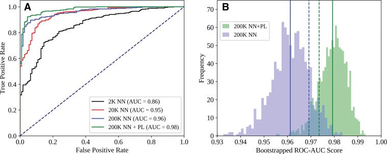
Comparisons between the ROC curves for the NN+PL and NN-type classifiers for each training set size can be found in Figure 3, A, while 1000-sample bootstrap frequencies for AUC values obtained from the NN+PL and NN classifiers are shown in Figure 3, B. The ROC for NN+PL was superior to that for NN alone at all points, and AUC values for a substantial majority of bootstrapped populations were greater for NN+PL than for NN alone. NN+PL also resulted in a smaller AUC variance than did NN alone.

Figure 3:

Comparison of, A, receiver operating characteristic (ROC) curves for DenseNet-121 (NN) and NN+PL (mean of NN score and prospective label [PL] score) classifiers and, B, area under the ROC curve (AUC) histograms obtained from a 1000-sample test set by using the bootstrap method. Each ROC curve represents the output of one representative NN model. In B, solid lines indicate mean values, and dashed lines indicate standard deviation from the mean. Data set size (K = 1000 points) refers to total size (training + development, 90-to-10 split).

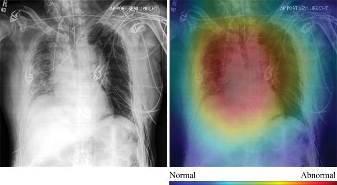
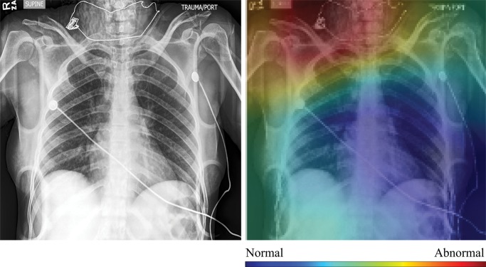
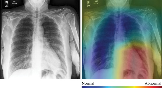
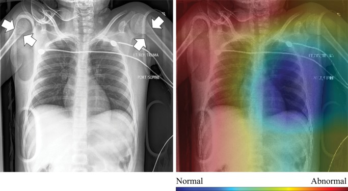
In Figure 4, we show selected examples of false-positive, false-negative, true-positive, and true-negative outputs, as determined by evaluating the DenseNet-121 classifier against the expert labels. These examples suggest that clinically meaningful spatial regions are influencing CNN classification, but they also show that it is critical in clinical practice to ensure that such a model only be used for the specific task for which it was designed.

Figure 4a:

High-resolution histogram-equalized images (left) and normalized class activation maps (CAMs) (224 × 224 resolution) (right) show (a) true-positive (decreased right lung volume; convolutional neural network [CNN] score 0.99), (b) false-positive (necklace; CNN score 0.57), (c) false-negative (borderline cardiomegaly; CNN score 0.48), and (d) true-negative (humerus fracture; CNN score 0.41) findings of thoracic disease. Red indicates areas of relatively high contribution to an abnormal score, while blue areas indicate the opposite. Because color information is normalized within each image, comparison of values across CAMs is not appropriate.

Discussion

Our results support several important observations regarding the use of CNNs for automated binary triage of chest radiographs, which to our knowledge has not been attempted at a comparable scale. For instance, we have shown that while carefully adjudicated image labels are necessary for evaluation purposes, prospectively labeled single-annotator data sets of a scale modest enough (approximately 20 000 samples) to be available to many institutions are sufficient to train high-performance classifiers for this task. These scalability results are in line with those of Gulshan et al (27), who found that CNN performance for classification of retinal fundus photographs reached a plateau after approximately 60 000 images. Furthermore, we observed that quantitative combination of the CNN score and clinician binary labels results in a tunable classifier that performs more similarly to expert radiologists, as measured with both AUC and Cohen κ values, than does either the CNN or the clinician alone.

Our study showed the utility of noisier (or “weaker”) sources of supervision in radiologic classification tasks. Specifically, CNNs in our study are trained by using a large prospectively labeled data set that contains label noise that results not only from occasional disagreement between the attending physician and expert consensus, but also from a variety of factors that affect clinical practice, such as erroneous prospective label entry (which would not affect triage outcome), inconsistent application of the prospective label protocol across more than 30 faculty members in six subspecialty divisions in the department over nearly 15 years, and clinician use of information not contained within the image. Although CNNs were trained with this noisier data set, CNN model results show more similarity with expert labelers than with noisier prospective labels, as measured with both AUC and κ statistics. These trends align with those described in the growing literature on weak supervision, which has shown that end-model performance can asymptotically improve with data set size, even when noisy sources of supervision are used (28,29). Ultimately, the fact that larger noisier label sets can be used to train models that perform well when evaluated against expert assessments could enable the creation of useful machine learning models from existing data for a variety of medical use cases. As expected, model evaluation against noisier prospective labels rather than against expert-provided labels led to lower computed performance metrics, emphasizing the need for confident labels for model assessment.

Qualitative evaluation of model behavior via the paired images and CAMs in Figure 4, along with associated text reports, also yields useful insight into both success and failure modes of these models. In the true-positive example shown in Figure 4a, the CNN is correctly influenced by pixels covering the collapsed right lung. The false-positive example shown in Figure 4b is interesting because the patient’s necklace, which represents an uncommon thin high-attenuation object, seems to contribute substantially to the positive rating; this case is indicative of the wide variety of error modes that can occur in this task. Note that false-positive findings made up the majority of model errors and consisted of 24% borderline cases; 27% containing support devices, such as feeding tubes; 21% misclassified normal examinations; and 28% miscellaneous mild conditions (eg, shoulder arthritis) not deemed abnormal for thoracic disease by the expert panel.

Figure 4b:

High-resolution histogram-equalized images (left) and normalized class activation maps (CAMs) (224 × 224 resolution) (right) show (a) true-positive (decreased right lung volume; convolutional neural network [CNN] score 0.99), (b) false-positive (necklace; CNN score 0.57), (c) false-negative (borderline cardiomegaly; CNN score 0.48), and (d) true-negative (humerus fracture; CNN score 0.41) findings of thoracic disease. Red indicates areas of relatively high contribution to an abnormal score, while blue areas indicate the opposite. Because color information is normalized within each image, comparison of values across CAMs is not appropriate.

Further, the attending physician noted mild cardiomegaly in the false-negative example shown in Figure 4c. Here, the model was correctly influenced by the lower left cardiac region, and the relatively high CNN score for this negative example (0.48) indicated that both the CNN and the physician evaluated this study as borderline abnormal. Finally, the true-negative image shown in Figure 4d is a particularly good example of how interpretation of model output must be performed in an appropriate context. Although both the model and the expert labelers indicated no thoracic disease, the clinical report described and the image showed bilateral proximal transverse humeral metaphyseal fractures, which represent a serious clinical condition. Given that humeral fractures are rare on chest radiographs, it is not surprising that the CNN would not recognize this injury. Thus, while the CAMs provide compelling evidence that CNN classification is most heavily influenced by clinically relevant spatial regions, they also show that these models will not necessarily generalize beyond the thoracic triage task for which they were trained. Additional examples for each success and failure mode can be found in Appendix E1 (online).

Figure 4c:

High-resolution histogram-equalized images (left) and normalized class activation maps (CAMs) (224 × 224 resolution) (right) show (a) true-positive (decreased right lung volume; convolutional neural network [CNN] score 0.99), (b) false-positive (necklace; CNN score 0.57), (c) false-negative (borderline cardiomegaly; CNN score 0.48), and (d) true-negative (humerus fracture; CNN score 0.41) findings of thoracic disease. Red indicates areas of relatively high contribution to an abnormal score, while blue areas indicate the opposite. Because color information is normalized within each image, comparison of values across CAMs is not appropriate.

Figure 4d:

High-resolution histogram-equalized images (left) and normalized class activation maps (CAMs) (224 × 224 resolution) (right) show (a) true-positive (decreased right lung volume; convolutional neural network [CNN] score 0.99), (b) false-positive (necklace; CNN score 0.57), (c) false-negative (borderline cardiomegaly; CNN score 0.48), and (d) true-negative (humerus fracture; CNN score 0.41) findings of thoracic disease. Red indicates areas of relatively high contribution to an abnormal score, while blue areas indicate the opposite. Because color information is normalized within each image, comparison of values across CAMs is not appropriate.

Our study had several limitations. First, model performance is better for the abnormal class than for the normal class, even when trained with data sets balanced by undersampling. This implies that the task of identifying the absence of disease or injury can be difficult, as expected. Further, absolute performance could potentially be improved by additional architecture and hyperparameter searches, threshold tuning, model ensembling, or data augmentation. We did not emphasize these well-known techniques in our study; instead, we focused on demonstrating viability and assessing trends rather than on optimizing end performance. Additionally, given that our data for both training and testing were sourced from the same institution, it remains an open question as to whether the models presented here can be generalized to data from other institutions, which may have different data preparation techniques or population statistics that could lead to higher error rates (30). Our results, however, suggest that only moderately large numbers of images (on the order of tens of thousands) are needed to train institution-specific models that have clinically useful performance. Indeed, the ability of CNN-based architectures to interpolate the data, rather than to learn features that can be generalized to other data sets, may be sufficient for them to provide practical utility. Finally, we noted that images were downsampled to 224 × 224 pixels to assess the performance of standard pretrained CNNs from computer vision for this radiograph classification task; future work should address the utility of domain-specific CNN architectures that could leverage additional information in the high-resolution image.

In conclusion, we found that CNNs trained by using a modestly sized corpus of prospectively labeled chest radiographs show promise in performing automated chest radiograph triage at levels that may be useful in clinical practice, attaining AUC values of up to 0.96 with respect to expert labels. Such a system could provide value in many clinical contexts, including workflow prioritization in undersourced clinics and automated triage in areas without access to trained radiologists. Further, the fact that the tradeoff between classifier sensitivity and specificity is more favorable at every possible operating point when the output of the CNN is averaged with the prospective label suggests that even relatively simple combined human and artificial intelligence systems could improve performance for real-world radiologic interpretation tasks. The results of our study should be validated in other patient populations; however, our findings suggest a distinct value to combining deep-learning techniques, such as CNNs, with data sets of sizes already accessible to many institutions to improve thoracic imaging triage.

References

- 1.Rimmer A. Radiologist shortage leaves patient care at risk, warns royal college. BMJ 2017;359:j4683. [DOI] [PubMed] [Google Scholar]
- 2.Bastawrous S, Carney B. Improving patient safety: avoiding unread imaging exams in the national VA enterprise electronic health record. J Digit Imaging 2017;30(3):309–313. [DOI] [PMC free article] [PubMed] [Google Scholar]
- 3.Rosman DA, Nshizirungu JJ, Rudakemwa E, et al. Imaging in the land of 1000 hills: Rwanda radiology country report. J Glob Radiol 2015;1(1):6. [Google Scholar]
- 4.Ali FS, Harrington SG, Kennedy SB, Hussain S. Diagnostic radiology in Liberia: a country report. J Glob Radiol 2015;1(1):6. [Google Scholar]
- 5.LeCun Y, Bengio Y, Hinton G. Deep learning. Nature 2015;521(7553):436–444. [DOI] [PubMed] [Google Scholar]
- 6.Deng J, Dong W, Socher R, Li LJ, Li K, Li F. ImageNet: a large-scale hierarchical image database. In: IEEE CVPR 2009; 248–255. [Google Scholar]
- 7.Spampinato C, Palazzo S, Giordano D, Aldinucci M, Leonardi R. Deep learning for automated skeletal bone age assessment in x-ray images. Med Image Anal 2017;36:41–51. [DOI] [PubMed] [Google Scholar]
- 8.Larson DB, Chen MC, Lungren MP, Halabi SS, Stence NV, Langlotz CP. Performance of a deep-learning neural network model in assessing skeletal maturity on pediatric hand radiographs. Radiology 2018;287(1):313–322. [DOI] [PubMed] [Google Scholar]
- 9.Lee H, Tajmir S, Lee J, et al. Fully automated deep learning system for bone age assessment. J Digit Imaging 2017;30(4):427–441. [DOI] [PMC free article] [PubMed] [Google Scholar]
- 10.Hua KL, Hsu CH, Hidayati SC, Cheng WH, Chen YJ. Computer-aided classification of lung nodules on computed tomography images via deep learning technique. OncoTargets Ther 2015;8:2015–2022. [DOI] [PMC free article] [PubMed] [Google Scholar]
- 11.Lakhani P, Sundaram B. Deep learning at chest radiography: automated classification of pulmonary tuberculosis by using convolutional neural networks. Radiology 2017;284(2):574–582. [DOI] [PubMed] [Google Scholar]
- 12.Anavi Y, Kogan I, Gelbart E, Geva O, Greenspan H. A comparative study for chest radiograph image retrieval using binary texture and deep learning classification. In: 2015 37th Annual International Conference of the IEEE Engineering in Medicine and Biology Society (EMBC).IEEE, 2015; 2940–2943. [DOI] [PubMed] [Google Scholar]
- 13.Rajkomar A, Lingam S, Taylor AG, Blum M, Mongan J. High-throughput classification of radiographs using deep convolutional neural networks. J Digit Imaging 2017;30(1):95–101. [DOI] [PMC free article] [PubMed] [Google Scholar]
- 14.Lakhani P. Deep convolutional neural networks for endotracheal tube position and x-ray image classification: challenges and opportunities. J Digit Imaging 2017;30(4):460–468. [DOI] [PMC free article] [PubMed] [Google Scholar]
- 15.Wang X, Peng Y, Lu L, Lu Z, Bagheri M, Summers RM. ChestX-ray8: Hospital-scale Chest X-ray Database and Benchmarks on Weakly-Supervised Classification and Localization of Common Thorax Diseases. In: IEEE CVPR 2017; 3462–3471. [Google Scholar]
- 16.Lehman CD, Wellman RD, Buist DS, et al. Diagnostic accuracy of digital screening mammography with and without computer-aided detection. JAMA Intern Med 2015;175(11):1828–1837. [DOI] [PMC free article] [PubMed] [Google Scholar]
- 17.Davies ER. Computer and machine vision: theory, algorithms, practicalities. Waltham, Mass: Academic Press/Elsevier, 2012. [Google Scholar]
- 18.Krizhevsky A, Sutskever I, Hinton GE. ImageNet classification with deep convolutional neural networks. Commun ACM 2012;60(6):84–90 [Google Scholar]
- 19.He K, Zhang X, Ren S, Sun J. Deep residual learning for image recognition. In: IEEE CVPR 2016; 770–778. [Google Scholar]
- 20.Huang G, Liu Z, Van Der Maaten L, Weinberger KQ. Densely connected convolutional networks. In: IEEE CVPR 2017;3:4700–4708. [Google Scholar]
- 21.Paszke A, Gross S, Chintala S, et al. Automatic differentiation in PyTorch. Neural Inf Process Syst Autodiff Work, 2017. https://openreview.net/forum?id=BJJsrmfCZ. Accessed May 8, 2018.
- 22.Vedaldi A, Zisserman A. Efficient additive kernels via explicit feature maps. IEEE Trans Pattern Anal Mach Intell 2012;34(3):480–492. [DOI] [PubMed] [Google Scholar]
- 23.Vedaldi A, Fulkerson B. VLFeat: an open and portable library of computer vision algorithms. In: Proceedings of the 18th ACM international conference on Multimedia, 2010; 1469–1472. [Google Scholar]
- 24.DeLong ER, DeLong DM, Clarke-Pearson DL. Comparing the areas under two or more correlated receiver operating characteristic curves: a nonparametric approach. Biometrics 1988;44(3):837–845. [PubMed] [Google Scholar]
- 25.Hanley JA, McNeil BJ. A method of comparing the areas under receiver operating characteristic curves derived from the same cases. Radiology 1983;148(3):839–843. [DOI] [PubMed] [Google Scholar]
- 26.Zhou B, Khosla A, Lapedriza A, Oliva A, Torralba A. Learning deep features for discriminative localization. In: IEEE CVPR 2016; 2921–2929. [Google Scholar]
- 27.Gulshan V, Peng L, Coram M, et al. Development and validation of a deep learning algorithm for detection of diabetic retinopathy in retinal fundus photographs. JAMA 2016;316(22):2402–2410. [DOI] [PubMed] [Google Scholar]
- 28.Ratner A, De Sa C, Wu S, Selsam D, Ré C. Data programming: creating large training sets, quickly. Adv Neural Inf Process Syst 2016;29:3567–3575. [PMC free article] [PubMed] [Google Scholar]
- 29.Ratner A, Bach SH, Ehrenberg H, Fries J, Wu S, Ré C. Snorkel: rapid training data creation with weak supervision. Proceedings VLDB Endowment 2017;11(3):269–282. [DOI] [PMC free article] [PubMed] [Google Scholar]
- 30.Park SH, Han K. Methodologic guide for evaluating clinical performance and effect of artificial intelligence technology for medical diagnosis and prediction. Radiology 2018;286(3):800–809. [DOI] [PubMed] [Google Scholar]
- 31.Kingma DP, Ba JL. Adam: a method for stochastic optimization. In: International Conference on Learning Representations 2015. https://pdfs.semanticscholar.org/aeea/02a93d674e0a044a8715e767f3a372582604.pdf. Published 2015. Accessed March 31, 2018. [Google Scholar]
Associated Data
This section collects any data citations, data availability statements, or supplementary materials included in this article.