

Abstract
We analyzed a large health insurance dataset to assess the genetic and environmental contributions of 560 disease-related phenotypes in 56,396 twin pairs and 724,513 sibling pairs out of 44,859,462 individuals that live in the United States. We estimated the contribution of environmental risk factors (socioeconomic status, air pollution, and climate) in each phenotype. Mean heritability (h2 = 0.311) and shared environmental variance (c2 = 0.088) were higher than variance attributed to specific environmental factors such as zip code-level socioeconomic status (SES) (varSES = 0.002), daily air quality (varAQI = 0.0004), and average temperature (vartemp = 0.001) overall, as well as for individual phenotypes. We found significant heritability and shared environment for a number of comorbidities (h2 = 0.433, c2 = 0.241) and average monthly cost (h2 = 0.290, c2 = 0.302). All results are available using our “Claims Analysis of Twin Correlation and Heritability (CaTCH)” web application.
Editorial summary:
Analysis of a health insurance dataset comprising over 44 million individuals allows for the estimation of genetic and environmental contributions in 560 phenotypes using twins and sibling pairs.
Introduction
Disentangling how genetic and environmental factors contribute to many phenotypes in the same population has been largely unfeasible to date. Most study designs consider a single disease or environmental factor at a time. Large administrative health datasets are an emerging stream of health data that enables more comprehensive analysis involves large administrative health data. Here, we analyze a massive, individual-level claims dataset of 44,859,462 individuals to systematically partition phenotypic variance between genetic and non-genetic factors across a large U.S. population. Documenting both the genetic and environmental contributions of phenotypic variance is instrumental for major health studies, such as the United States’ All of Us effort1,2. Furthermore, the use of genome sequence data in medical decision making is under debate2 and estimating heritability in a “real world” setting can help quantify the clinical utility of genome sequencing3.
In human genetics, heritability is defined as the amount of phenotype or disease variation that can be attributed to genetic factors. In family studies, other important quantities, such as “shared environment” and “non-shared environment” complement heritability and quantify variation in phenotype due to non-genetic factors. Estimation of heritability and environmental components of phenotypic variation have historically used family-based studies, such as those involving twins that are concordant (and discordant) for disease. However, building twin registries can be resource-intensive in the ascertainment of both twin pairs and phenotypes. What is missing are family-based studies that measure numerous phenotypes across a large and diverse population that experience a variety of environmental exposures. First, health administration data enable such an approach because these data give a comprehensive snapshot of health (e.g., thousands of disease diagnoses and laboratory reports, in addition to cost of healthcare), and they enable family-based4,5 or twin-based studies across a large number of diseases. While twin-based analysis in such datasets is difficult due to lack of zygosity information, we employ methodology6 that utilizes sex information to differentiate between identical and non-identical twin pairs.
Second, there has also been a great deal of interest in understanding the contribution of one’s residence or zip code to their disease state7. Patient-level data with geographical and temporal information (i.e., patient mailing zip code and time of diagnosis) can enable an understanding of the contribution of specific geographically linked environmental factors to phenotypic variation. There is growing interest in understanding whether one’s residence (i.e., zip code) or genetic “code” is more important in health8 but, to our knowledge, only one study has attempted to quantify the relative contribution of local environment and genetics9. In our analysis, we quantify the relative contribution of local environment and genetics by integrating individual-level data with zip code-level information that serve as geographical indicators of the area’s socioeconomic status, air pollution quality level, and weather/climate. We then estimated heritability, shared environment, and contribution of zip code specific environmental factors for 551 disease-related phenotypes.
We estimated heritability and shared environmental variance for 560 phenotypes (based on diagnostic billing codes and laboratory tests) in a cohort of 56,396 twin pairs born on or after 1985 (individuals that are on their parent’s/guardian’s insurance plan) using an individual-level claims dataset of 44,859,462 individuals from the United States. We also estimated phenotypic correlation for same sex and opposite sex siblings using a cohort of 724,513 sibling pairs (Supplementary Note). We estimated the contribution of specific environmental risk factors such as socioeconomic status, pollution, and climate to these phenotypes by linking individual claimants to external datasets via residential locations (Figure 1d-g). In addition, we computed genetic and environmental contributions of cost of care utilization and total co-morbidities. Finally, we estimated the validity of our estimates for heritability and shared environment through systematic comparison of documented estimates in the published literature.
Figure 1: Geographic distribution of 56,396 twin pairs in CaTCH and example of environmental data aggregation on a zip code basis.
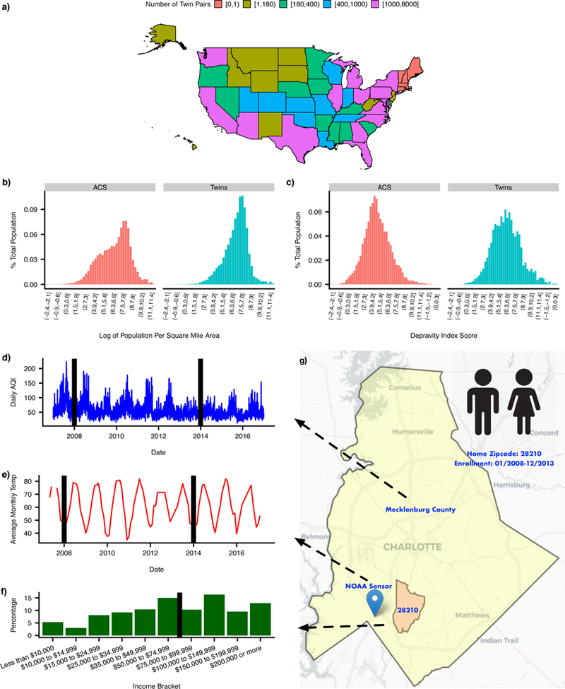
(a) Count of twin pairs in CaTCH for each state in the United States. (b) Distribution of log of population density for the entire United States and twin pairs. (c) Distribution of depravity index for the entire United States and twin pairs. (d) Time series for daily AQI for Mecklenburg county. Black lines represents years 2008 and 2014, respectively. (e) Time series for average monthly temperature for NOAA sensor closest to zip code 28210. Black lines represents years 2008 and 2014, respectively. (f) Distribution of median family income distribution among residents of zip code 28210. Black line represents mean median income value. (g) Map of county, zip code, and closest NOAA sensor for hypothetical twin pair residing in zip code 28210. Background map image from OpenStreetMap licensed under Creative Commons Attribution-ShareAlike 2.0 license (CC BY-SA). (NOAA - National Oceanic and Atmospheric Administration; AQI - air quality index)
Results
Data overview
We utilized de-identified member claims data from Aetna Inc., a national health insurance company, to assemble a cohort of 56,396 twin pairs and 724,513 sibling pairs (Online Methods and Supplementary Note) that were members for at least 3 years in the period between 01/01/2008 - 02/01/2016. The median age of twin and sibling pairs at the start of surveillance was 7 years (Table 1). The age range for twins and siblings in this cohort was between 0-24 years. Using the claims data, we mapped health claims codes to higher level phenotypes called PheWAS codes10 (Online Methods). Phenotypic filtering produced 551 PheWAS codes, 7 quantitative phenotypes, and 2 derived quantitative phenotypes. The twin cohort was geographically heterogeneous. There were 38 states with at least 100 twin pairs, while 6 states had no twin pairs (Figure 1a). Overall, the twin pairs resided in areas with higher income and population density (Figure 1b-c). Prevalence of PheWAS phenotypes, among twin pairs, was variable within and between different functional domains [prevalence = 0.30% - 73.2%] (Supplementary Figure 1). All results, including phenotype specific data, are available using our “Claims Analysis of Twin Correlation and Heritability (CaTCH)” web application (see URLs).
Table 1:
Characteristic of ascertained insurance claims twin and sibling cohorts
| All Pairs | FF Pairs | MM Pairs | MF Pairs | |
|---|---|---|---|---|
| Number of twin pairs | 56,396 | 17,835 | 17,919 | 20,642 |
| Number of sibling pairs | 724,513 | 171,095 | 187,033 | 366,385 |
| Median age at start of surveillance (IQR) (twin) | 7 (3-13) | 8 (3-14) | 8 (3-13) | 7 (2-12) |
| Median age at start of surveillance (IQR) (sibling) | 7 (2-12) | 7 (2-12) | 7 (2-12) | 7 (2-12) |
| Median months of surveillance (IQR) (twin) | 60 (45-84) | 60 (45-84) | 60 (45-84) | 60 (45-84) |
| Median months of surveillance (IQR) (sibling) | 61 (46-84) | 61 (46-84) | 61 (46-84) | 61 (46-84) |
| Median number of ICD Codes (IQR) (twin) | 23 (12-42) | 23 (12-41) | 22 (11-41) | 24 (13-44) |
| Median number of ICD Codes (IQR) (sibling) | 23 (12-42) | 24 (13-42) | 22 (11-41) | 23 (12-42) |
| Distinct number of zip codes (twin) | 11,666 | 7,302 | 7,235 | 7,466 |
| Distinct number of zip codes (sibling) | 24,703 | 17,324 | 17,606 | 21,112 |
| Surveillance period | 01/01/2008 - 02/01/2016 | |||
FF Pairs, twin pairs where both individuals are female; MM Pairs, twin pairs where both individuals are male; MF pairs, twin pairs where one individual is male and the other is female.
Estimation of h2 and c2
We used a twin-based method to estimate the proportion of phenotypic variance due to additive genetic factors (i.e. the narrow-sense heritability, h2) and variance due to environmental factors shared between twins (c2). Due to lack of zygosity information, we estimated h2 and c2 using the difference in correlation between same sex (rtwinSS) and opposite sex twin pairs (rtwinOS), assuming that opposite sex pairs are dizygotic and same sex twin pairs are a mixture of monozygotic and dizygotic twin pairs (Online Methods). We tested the validity of the assumption that rtwinOS is a good proxy for same sex dizygotic twin correlation (rtwinDZSS) by creating a sibling cohort and estimating the correlation between same sex sibling correlation (rsibSS) and opposite sex sibling correlation (rsibOS) for all 551 binary phenotypes (Supplementary Note). We found rsibSS and rsibOS were highly correlated ( = 0.978, 95% CI: [0.974, 0.981]) (Supplementary Figure 2). Also, for 95% of phenotypes, rsibSS - rsibOS ranged between −0.012 and 0.051 and rsibSS was, on average, 0.017 higher than rsibOS (Supplementary Figure 3), but for 23.5% of phenotypes rsibSS - rsibOS followed the null distribution (pi0 statistic11). We conclude that rtwinOS is highly correlated with rtwinDZSS for these 551 phenotypes. However, we found that rtwinOS is slightly lower, on average, than rtwinDZSS. Therefore, the estimates of h2 and c2 will be slightly biased. We also found rtwinOS is, in general, larger than both rsibOS and rsibSS (Supplementary Figure 4). Therefore, using rsibSS instead of rtwinOS as a proxy for rtwinDZSS simply replaces one biased estimator for another(Supplementary Note). We also found strong evidence to the validity of our assumption of Weinberg’s Rule (Supplementary Note).
Overall phenome-wide summary of h2 and c2
The inverse-variance weighted mean estimate among all phenotypes was 0.316 (95% CI: [0.296, 0.335]) for h2 and 0.088 (95% CI: [0.074, 0.102]) for c2 (Figure 2a). Also, among all phenotypes, the opposite and same sex correlations for twins (rtwinSS = 0.307, 95% CI: [0.297, 0.318], rtwinOS = 0.240, 95% CI: [0.229, 0.251]) are higher than for the siblings (rsibSS = 0.199, 95% CI: [0.192, 0.206], rsibOS = 0.182, 95% CI: [0.175, 0.189]). The rtwinSS estimate is highest because same sex twin pairs are a mixture of monozygotic and dizygotic twin pairs. The higher value for rtwinOS compared to both rsibSS and rsibOS is due to a larger twin shared environment versus the sibling shared environmental effect.
Figure 2: Estimates of twin statistics across functional domains and individual basis for 56,396 twin pairs in CaTCH among all 560 phenotypes.
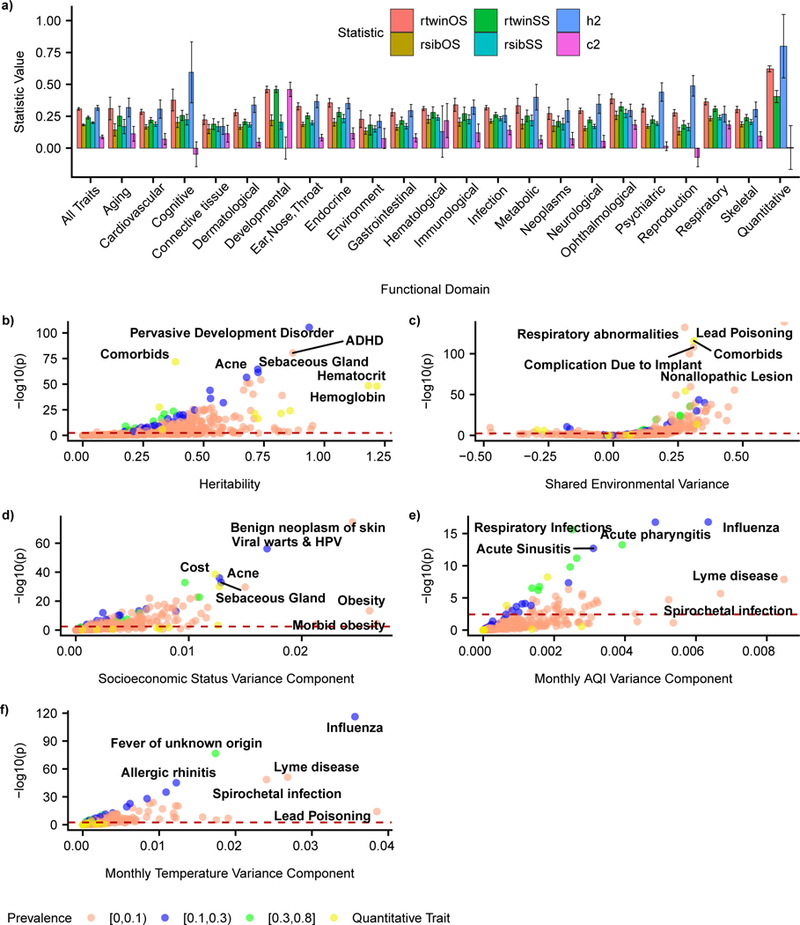
(a) Barplot of meta-analytic estimates of rtwinOS, rtwinSS, h2, and c2 among all 560 phenotypes and within functional domains for, error bars represent 95% CI. (b) - (f) Volcano plots for estimates of h2, c2, varSES, varAQI, and vartemp respectively along with labels for phenotypes with top p-values and large effect sizes for each estimate. Dashed red lines represents threshold for Benjamini-Yekutieli FDR adjusted p-values passing significance (p=0.05) for each estimate, respectively.
Accounting for multiple hypotheses by controlling the false discovery rate (FDR) at 5% we found 326/560 (58.2%) phenotypes had a non-zero heritability (h2 > 0) and 180/560 (32.1%) phenotypes had non-zero shared environmental effects (c2 > 0). Of these phenotypes, 225/560 (40%) h2 estimates and 138/560 (24.6%) c2 estimates remained significant at a more stringent significance level by Bonferroni-adjusted p-value < 0.05. We show a volcano plot of both h2 and c2 estimates for all 560 phenotypes, where the dotted line represents the FDR threshold for each statistic (Figure 2b-c). The majority of age () and sex () fixed effects were also non-zero (Online Methods, eq. 3). Controlling for multiple hypotheses using an FDR threshold of 0.05 there were 487/560 (86.9%) phenotypes for and 281/560 (50.1%) phenotypes for that were FDR significant, respectively (See URLs).
Among functional domains with at least 5 phenotypes, the domains with the highest h2 were quantitative laboratory measures (h2 = 0.799, 95% CI: [0.551,1.048], 7 out of 7 phenotypes reached FDR threshold) and cognitive (h2 = 0.594, 95% CI: [0.355, 0.834], 4 out of 5 phenotypes reached FDR threshold) (Figure 2a). The lowest were connective tissue (h2 = 0.170, 95% CI: [0.108, 0.233], 2 out of 11 phenotypes reached FDR threshold) and environment (h2 = 0.211, 95% CI: [0.161, 0.260], 24 out of 45 phenotypes reached FDR threshold) (Figure 2a).
The functional domains with highest c2 were ophthalmological (c2 = 0.183, 95% CI: [0.147, 0.218], 27 out of 42 phenotypes reached FDR threshold) and respiratory (c2 = 0.182, 95% CI: [0.151, 0.213], 34 out of 48 phenotypes reached FDR threshold) (Figure 2a). The lowest were reproduction (c2 = −0.073 95% CI: [−0.146, 0.000], 3 out of 18 phenotypes reached FDR threshold) and cognitive (c2 = −0.048, 95% CI: [−0.145, 0.049], 2 out of 5 phenotypes reached FDR threshold) (Figure 2a)
From all 560 phenotypes in this study, there were 294 phenotypes (52.5%) where c2 followed the null distribution (pi0 statistic11) (Online Methods), consistent with a model where twin resemblance was solely due to additive genetic variance.
Cost and comorbidities have significant h2 and c2
We found that average monthly cost had both significant h2 > 0 and c2 > 0 (Figure 3b) in the twin pairs. Specifically, the estimate of h2 was 0.290 (95% CI: [0.241, 0.339]) and 0.433 (95% CI: [0.390, 0.477]) for average monthly cost and number of PheWAS comorbidities, respectively. Estimates of c2 were comparable; c2 = 0.302, 95% CI: [0.271, 0.332] for average monthly cost and c2 = 0.241, 95% CI: [0.213, 0.268] for number of PheWAS comorbidities (Figure 3b). The same and opposite sex twin correlations (rtwinSS and rtwinOS) for number of PheWAS comorbidities (rtwinSS = 0.549, 95% CI: [0.543, 0.556], rtwinOS = 0.458, 95% CI: [0.450, 0.465]) were slightly higher than average monthly claims cost (rtwinSS = 0.508, 95% CI: [0.501, 0.515], rtwinOS = 0.447, 95% CI: [0.439, 0.455]) (Figure 3b).
Figure 3: Comparison of h2 estimates in CaTCH to published literature and estimates for cost and comorbidities in CaTCH.

(a) Scatterplot of published h2 estimates from 56,396 twin pairs in CaTCH versus h2 estimates from 81 published studies, vertical and horizontal error bars are 95% CI for CaTCH and published estimates respectively, black line is line with slope 1 and intercept 0, blue line is line of best fit, and gray shaded region is 95% CI for line of best fit. (b) Barplot of estimates of h2, c2, rtwinOS, and rtwinSS for phenotypes Average Monthly Cost and Number of PheWAS comorbidities from 56,396 twin pairs, error bars represent 95% CI.
Specific geocoded environmental factors
In the same model, we estimated the proportion of variance in a phenotype attributable to environmental risk factors (based on home zip code), including a socioeconomic status (SES) “index” (Supplementary Note) (varSES), median air quality index exposure (varAQI), and median monthly average temperature exposure (vartemp) in addition to h2 and c2. The variance components for environmental risk factors were modest compared to h2 and c2. For all phenotypes varSES = 0.002 (95% CI: [0.002, 0.002]), varAQI = 0.0001 (95% CI: [0.0003, 0.0005), and vartemp = 0.001 (95% CI: [0.001, 0.001]), much smaller than the mean estimates of h2 and c2 described earlier (Supplementary Figure 5). Controlling for multiple hypotheses using an FDR threshold of 0.05 there were 145/560 phenotypes for varSES, 36/560 phenotypes for varAQI, and 117/560 phenotypes for vartemp that passed FDR significance. Phenotypes with largest varSES were morbid obesity (varSES = 0.027, 95% CI: [0.014, 0.039]) and benign neoplasm of skin (varSES = 0.024, 95% CI: [0.022, 0.027]). Phenotypes with largest varAQI were Lyme disease (varAQI = 0.008, 95% CI: [0.006, 0.011]) and average monthly cost (varAQI = 0.006, 95% CI: [0.004, 0.009]). Phenotypes with largest vartemp were lead poisoning (vartemp = 0.039, 95% CI: [0.029, 0.048]) and influenza (vartemp = 0.036, 95% CI: [0.033, 0.039]) (Figure 2d-f).
Comparison to published literature
We compared our estimates of h2 and c2 to a large meta-analysis of twin studies (MaTCH), containing 9,568 phenotypes from 5,169,879 twin pairs where monozygotic and dizygotic correlation were reported. The two major differences between CaTCH and MaTCH were CaTCH studied 38 infectious diseases compared to MaTCH and the CaTCH cohort was younger than most of the studies in MaTCH (Supplementary Note).
Comparing the CaTCH estimates to MaTCH estimates, we observed mean claims heritability (h2 = 0.315; (95% CI: [0.296, 0.334]) was smaller than the mean MaTCH estimate (h2 = 0.593, 95% CI: [0.577, 0.608]) (Figure 4a). Further, the mean CaTCH shared environment (c2 = 0.088, 95% CI: [0.074, 0.102]) was higher than the mean MaTCH estimate (c2 = 0.042, 95% CI: [0.028, 0.055]) (Figure 4b) 12. Comparing CaTCH h2 estimates with MaTCH h2 estimates along functional domains, we observed overlap between the 95% CI from h2 CaTCH estimates and 95% CI from h2 MaTCH estimates for 7 out of 21 functional domains, namely cognitive, endocrine, environment, hematological, infection, psychiatric, and reproduction functional domains (Figure 4a). For c2 the 95% CI from CaTCH estimates overlapped with the 95% CI from the MaTCH estimates for only the infection domain (Figure 4b). In the MaTCH analysis, 69.1% of phenotypes are consistent with a model where twin resemblance was due solely to additive genetic variance12 compared to 52.5% of phenotypes in CaTCH.
Figure 4: Comparison of h2/c2 estimates from 56,396 twin pairs among 560 phenotypes in CaTCH to 5,169,880 twin pairs among 9,568 phenotypes in MaTCH (Supplementary Table 1).
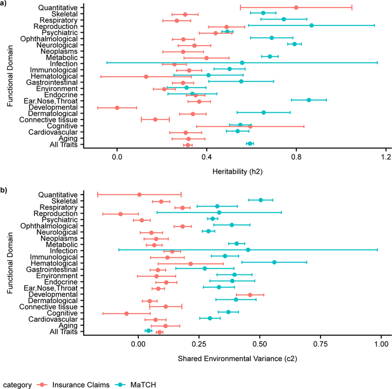
(a) Meta-analytic h2 estimates for all phenotypes and functional domains between CaTCH and MaTCH, error bars represent 95% CI. (b) Meta-analytic c2 estimates for all phenotypes and functional domains between MaTCH and CaTCH, error bars represent 95% CI.
While we observed differences in heritability between CaTCH and MaTCH for aggregate phenotypic categories, we observed concordance when comparing individual phenotypes. We compared our CaTCH estimates to published estimates from the literature on an individual phenotype basis (Supplementary Note). We found the correlation for 81 binary and quantitative phenotypes between CaTCH estimates and the published literature was high, r = 0.817 (95% CI: [0.493, 1.14]) (Figure 3a). We also found 67/81 (82.7%) of phenotypes to have overlapping 95% confidence intervals. Of the 81 phenotypes, 49/81 (60.5%) were higher in the published literature.
Discussion
Here, we have used a large insurance claims dataset to systematically investigate the genetic and environmental contributions in phenotypic variation of 560 phenotypes, including specific environmental risk factors such as socioeconomic status, pollution exposure, and climate. Furthermore, we provide the first estimates of the contributions of genetics and environment in aggregate health cost and co-morbidity burden, important for both biological research and policy implementation. We also quantified the contribution of one’s genetic code and aspects of one’s zip code (socioeconomic status, climate, and air pollution) on the same scale of phenotypic variation for 551 disease-related phenotypes, by linking to external geographic databases.
A notable strength of our study was the creation of a large twin cohort. To the best of our knowledge, we amassed the largest twin cohort in the United States that is reflective of household, geographic, and medical service-based variation of the employed US population. The largest known US twin registries are the Mid-Atlantic Twin Registry (28,000 pairs) and Michigan State Twin Study (15,924). The largest international twin registries are from Sweden (97,000) and Denmark (85,000)13. Our twin cohort is comparable in size to these large international twin registries. Although, unlike some of these registries, we lack zygosity status for these twin pairs. Further, because we are using insurance claims data, our claims datasets contained the full transactional history between all medical providers and the insurance company for a particular patient. This includes all ICD 9/10 billing codes sent from the medical provider to the insurance company in order to be reimbursed. We claim this provides a comprehensive view into a patient’s medical history. In contrast, electronic medical records (EMR), because they are a record of the medical examination process, may have deeper phenotypic information (e.g. laboratory notes, radiology reports, and x-ray images), but will have an incomplete medical history if the patient sees multiple medical providers.
Twin designs have lower sample size compared to other family-based designs but are better powered to estimate heritability14. However, leveraging the family-based design in a claims-based cohort is not without disadvantages. First, a common issue in insurance data includes a limited observational time window to ascertain phenotype. This can lead to ascertainment bias in phenotypes when siblings are of different ages. This is further exacerbated with analysis including parents and children where, due to age of onset, the same phenotypic code may represent different disease subtypes4. Second, in a family design, it has been shown that estimates of h2 will be biased15 if all sources of familial environmental variation are unaccounted (e.g. spousal correlation and sibling correlation). Recent family-based studies attempted to estimate some of this familial environmental variation4,5; however, limitations remain, such as the lack of interpretability of multiple types of “shared environment.”4. In contrast, twin studies have a simpler design thereby allowing a single parameter (c2) to account for all shared environment. Third, claims data do not consider that non-biological relationships can also occur when using next of kin information or subscriber relationships. There is a possibility that ‘ascertained’ nuclear families may contain step-children, adoptions, or half-siblings, however, this can be modeled using Census data and pedigree simulations4. By using both the inferred sibling relationship and that they must be born on the same day, we claim smaller chance of twins being biologically unrelated.
A major novelty of our analysis was the ability to compare variance components of specific environmental factors with standard measures used in family-based analysis such as heritability and shared environmental variance. We note that each twin pair has the same shared environment, but our analysis attempts to partition phenotypic variance further with several identified shared environmental factors (Online Methods, Eq. 7) which are common among groups of twin pairs. We believe partitioning the shared environment into identified environmental factors (indicators of local SES, air pollution, and climate) is akin to analysis in partitioning heritability among functional annotations2-4. We found that variance components due to specific environmental factors were significantly lower compared to h2 and c2 overall and within each functional domain (Supplementary Figure 5). Part of the reason could be due to choices in how to assess exposure of the environmental risk variables for each particular twin as well as choices in discretizing these variables. In our analysis, we selected environmental variables based on an individual’s home residence postal code (zip code) versus individual-level exposure data, which may dilute the influence of these variables on phenotypes. We are limited in our ability to answer (1) how many additional measured shared environmental or non-genetic factors contribute to phenotypic variation beyond geocoded variables and (2) our method requires as input discretized environmental factors. Furthermore, environmental factors may also influence phenotypes through prolonged exposure. In our study, we are underpowered to detect this signal due to the young age of our cohort. A natural extension of this research includes approaches to consider continuous environmental variables in these novel and large data streams.
Specific environmental factors played little role in variation of most phenotypes, but we found intriguing results for a few phenotypes. The phenotype with largest socioeconomic variance component was morbid obesity (varSES = 0.027, 95% CI: [0.014, 0.039]). For Lyme disease, the variance components of all three environmental risk factors passed FDR significance for the phenotype (varSES = 0.022, 95% CI: [0.015, 0.028], varAQI = 0.006, 95% CI: [0.004, 0.009], varSES = 0.028, 95% CI: [0.023, 0.033]). For lead poisoning, vartemp was FDR significant (vartemp = 0.029, 95% CI: [0.017, 0.042]).
In the United States, predictors of health care cost and chronically ill patients are of particular importance19. In a recent analysis20 of high-cost patients the researchers emphasize prediction of high cost patients is important, yet current prediction methods do not include any family history information. Our twin analysis concludes that 0.59 of variance for average monthly cost is explained by h2 and c2.
Compared to the published literature (as reported by MaTCH) the CaTCH cohort was both younger, and also has a different distribution of phenotypes. First, in MaTCH, monozygotic correlation, dizygotic correlation, heritability, and shared environmental variance all were smaller, on average, for phenotypes ascertained after adolescence12. When comparing h2 estimates on an individual trait basis the correlation was high (r = 0.817, 95% CI: [0.493, 1.14]). A prerequisite to our analysis is selection of phenotypes with a minimum prevalence threshold and removal of phenotypes with high gender imbalance. Second, we were able to estimate genetic and environmental variance in 38 infectious diseases, compared to only 8 phenotypes in MaTCH12; on the other hand, phenotypes in psychiatric, metabolic, and cognitive domains accounted for 51% of all twin studies analyzed in MaTCH12. Such differences in both population and phenotypic selection possibly contribute to differences in estimates versus MaTCH (while still maintaining high correlation for h2 phenotypes on an individual trait basis), but there may be other methodological differences (such as lack of zygosity information) that may contribute to differences. Our procedure provides an opportunity to investigate phenotypes with large c2, such as lead poisoning and retinopathy of prematurity (See URLs) whereas many twin studies select phenotypes based on a prior belief of a genetic contribution.
Data on patients from health claims lack zygosity information that is typically ascertained in standard twin registries; however, by amassing a large number of non-twin sibling pairs from the same dataset, we found that the opposite sex twin correlation was close to sibling correlations. For our method to be internally valid, we make the following claims. First, we assume that phenotypic correlation of OS sex twin pairs (rtwinOS) is equivalent to dizygotic same sex twin pairs (rtwinDZSS). Second, we estimate the proportion of same sex twin pairs are monozygotic by assuming opposite sex and same sex dizygotic twin pairs are equally likely (Online Methods,eq. 20). We tested the first claim by interrogating the concordance between same sex and opposite sex sibling correlations. We found rsibSS and rsibOS were highly correlated ( = 0.978, 95% CI: [0.974, 0.981]), and, on average, rsibSS was slightly higher than rsibOS (average rsibSS - rsibOS = 0.017) for the 560 phenotypes passing our filtering criterion (Supplementary Note) and for 23.5% of phenotypes rsibSS - rsibOS followed the null distribution. We conclude that, overall, rtwinOS is a proxy for rtwinDZSS. We note that rtwinOS is higher than rsibOS and rsibSS for most phenotypes, implying increased h2 and decreased c2 if rsibOS or rsibSS were substituted for rtwinOS for those traits. We claim that high correlation rsibSS and rsibOS is primarily due to two factors. First, our phenotypic selection procedure eliminated phenotypes with large imbalances of sex-specific prevalence. Second, we add in sex as a covariate (‘fixed-effect’) in order to adjust for the mean differences between males and females. If rtwinOS were replaced by rsibSS then for the majority of phenotypes the estimate of h2 would increase and c2 would decrease bringing up the possibility that the contribution of the environment may change when assessing siblings rather than twins. We also tested the assumption of using Weinberg’s Law and effect of IVF had little to no effect on h2/c2 estimates (Supplementary Note).
In our analysis, we ascertained twin pairs between the ages of 0 to 24. This selection criterion eliminated our ability to study late-onset diseases such as Parkinson’s and Alzheimer’s disease. As with any administrative dataset, there may be errors in ascertainment of phenotype; for example, doctors may not be sure whether a child has type 1 diabetes or type 2 diabetes and therefore may bill for both diseases and therefore the individual may be ascertained as having both diseases. Such bias may be reduced by applying phenotyping algorithms (e.g. for diabetes21) for each phenotype; however, only a limited number of such algorithms exist.
In summary, our results provide a comprehensive picture of the contribution of genetics and the environment to a large number of phenotypes. We have also estimated the contribution of specific environmental risk factors in phenotype. Our estimates provide a useful baseline for determining the potential of further genetic and/or epidemiological research for a number of phenotypes of clinical relevance, applicable and complementary to precision medicine efforts, such as All of US1.
Online Methods
Study Population
We obtained our data from un-identifiable member claims data from Aetna Inc, a national health insurance company. The claims dataset contained the ICD 9/10 billing codes of 44,859,462 members with an Aetna insurance plan from January 2008 to February 2016 (Supplementary Figure 6a). This was a nationally representative dataset; 26,713 of 41,739 US mail zip codes have at least 20 members. We extracted a twin and sibling cohort to estimate genetic and environmental contribution in 560 phenotypes (Supplementary Figure 6e-k). The twin and sibling cohort focused on younger individuals born on or after 1985 because, under current US health care law, they qualified as dependents on their parent’s insurance plans (Supplementary Figure 6b). In all of our analysis we selected members enrolled for at least 36 consecutive months in order to have a sufficient period of time for the ascertainment of their phenotypes (Supplementary Figure 6b).
Twin and Sibling Cohort Creation
We created the twin cohort by extracting primary subscribers and their dependents. Specifically, a primary subscriber would add ‘dependents’ to his/her policy (approximately 26.19% are sole subscribers) and dependent individuals were coded as ‘child’, ‘grandchild’, ‘spouse’, ‘domestic partner’, ‘legal dependent’, and ‘student’. We ascertained family structure in this dataset using the relationship between the primary subscriber and child dependents (Supplementary Figure 6f). We restricted family size to, at most, 15 members living in the same zip code in order to reduce the chance multiple families are merged together (average family size is 3.98) (Supplementary Figure 6e). Once family units were created, we further extracted twins by comparing the birthdate of child subscribers that are linked to the same primary subscriber. We selected families where there is only one twin pair and eliminated children that are part of a triplet or greater because our estimation of h2 and c2 assumed twin pairs are independent and not part of an extended pedigree (Supplementary Figure 6g).
We created a sibling cohort as a basis for comparison to our twin cohort. Like the twin cohort, the sibling cohort utilized dependent information from the primary subscriber in order to determine sibling pairs (Supplementary Figure 6j). The sibling cohort also included families where there were at most 15 members, individuals must be born on or before 1985, individuals were enrolled as members for at least 36 months, and each individual had at least 1 ICD9/10 code (Supplementary Figure 6b-d). The age difference between sibling pairs had to be at least 11 months and no more than 36 months (Supplementary Figure 6k). Also, for each family, a single sibling pair that meet these conditions was selected at random (Supplementary Figure 6k).
Comparison of Twin Cohort to National Population
We compare our twin cohort to the general population using American Community Survey Census data. In particular, we ascertained all twins that were members, for at least one year, between 2009-2013 and compared to the 2009-2013 American Community Survey (ACS) estimates. Using census data, we estimated a measure for socioeconomic status for each zip code called the depravity index, a measure widely used in epidemiological literature22 (Supplementary Note). The depravity index is a measure of socioeconomic status for a zip code based on 7 census variables which were extracted from the 2009-2013 American Community Survey (See URLs). High depravity index values correspond to higher SES status and vice-versa. For all individuals in the 2009-2013 ACS we estimated their population density (log transform of number of people per square mile) and depravity index based on their home zip code and compare to the population density and depravity index of all twins, enrolled between 2009-2013, based on their home zip code. We observed that more twin pairs live in high population density areas compared to the general population (Figure 1b). The SES status of twin pairs, based on their home zip code, is slightly higher than the general US population (Figure 1c).
Phenotype Ascertainment
The claims dataset contained all International Classification of Disease (ICD) version 9/10 (hereafter ICD9/10 respectively) billing and diagnostic codes provided by the healthcare provider to the insurance company (Aetna, Inc) for transactional purposes while the individual was a subscriber to the health plan. In practice, many ICD9/10 codes may represent the same overarching phenotype, e.g. ICD 250.00 represents type 2 diabetes that is controlled, while 250.02 is type 2 diabetes that is uncontrolled. Therefore, we used PheWAS code groupings10. PheWAS codes are a way of combining ICD9 codes, used for phenotype-wide association studies10. Multiple ICD9/10 codes are combined into a single “phenotype”. Specifically, an individual was identified as positively having a PheWAS phenotype if they had at least one ICD 9/10 code from the PheWAS code grouping e.g. ICD 9 codes 250.00 and 250.02 both mapped to PheWAS code 250.2 type 2 diabetes. For rarer phenotypes, we utilized the groupings found in Blair, Rzhetsky et al.23 (we will collectively refer to these phenotypes as PheWAS codes). In total, we mapped Aetna subscriber ICD9/10 diagnostic codes to 1,900 PheWAS codes (Supplementary Figure 6c). PheWAS mappings were originally constructed using ICD9 codes, but the surveillance period for the insurance data spanned the transition from ICD9 to ICD10. In order to accommodate ICD10 codes, we utilized the United States Center for Disease Control and Prevention 2016 General Equivalence Mapping of ICD10 (see URLs) codes to ICD9 and subsequently to PheWAS codes.
For a subset of individuals, the claims dataset provided results of diagnostic clinical laboratory tests (hereafter called ‘lab test’) conducted during the individual’s medical care (Supplementary Figure 6c). Each lab test was identified by a LOINC code24. For only the twin cohort, we ascertained all lab tests where twin pairs were measured on the same day. In our analysis we included all laboratory tests where there were at least 2,000 twin pairs that match our criterion. The phenotypes we analyzed include common laboratory tests such as LDL cholesterol, HDL cholesterol, triglycerides, leukocyte counts, and hemoglobin counts. If a twin pair had multiple lab tests, then we randomly sampled a single lab test event for analysis.
Out of a total of 1,900 binary phenotypes, we removed phenotypes with low prevalence or where disparity in male and female prevalence was high (Supplementary Figure 6d) among twin pairs. In particular, for each phenotype, we imposed a filtering criterion where the ratio of male prevalence to female prevalence (or female to male prevalence) among twin pairs must be less than 5 (Supplementary Figure 6d). Also, only phenotypes with a prevalence of at least 0.3% were kept, resulting in phenotypes where at least 338 cases were expected and at least one concordant same sex (SS) and opposite sex (OS) pair allowing for stable estimation of h2 and c2, resulting in 551 binary phenotypes. In the case of the quantitative phenotypes, we analyzed lab value that had at least 2,000 twin pairs (Supplementary Figure 6d). For the sibling pairs, we ascertained only the 551 binary phenotypes.
For the twin cohort, within the claims dataset, we utilized an opportunity to derive phenotypes based on aggregate claims, including the total number of PheWAS codes per individual (or, ‘comorbidities’), and the average monthly cost incurred per individual (hereafter called ‘average monthly cost’). The number of PheWAS codes was the number of distinct PheWAS codes ascertained for a patient during the time of surveillance (at least 36 months) and can be thought of as the total number of ‘co-morbidities’ coded for each individual. Average monthly cost was the total claim costs divided by the months that the individual was a member of this insurance company when the costs were incurred.
Specific Environmental Risk Factors
For each twin pair we ascertained their home zip code and linked to census data depravity index, daily air quality index data, and monthly average temperature data. The depravity index is a composite score of socioeconomic status for a zip code based on 7 variables from the 2009-2013 American Community Survey (Supplementary Note). The EPA used the air quality index (AQI) to summarize air pollution level in a particular location. The AQI has a range between 0 and 500. An AQI value between 0-50 is considered good air quality, 50-100 is moderate air quality, and above 100 is considered unhealthy air quality. We downloaded all daily county-level AQI data provided by the EPA (see URLs) and estimated the median AQI level exposure for each twin pair based on the twin pairs dates of enrollment and closest county to their zip code (maximum distance of 30 km) (Figure 1d). We also ascertained all monthly average temperature data from sensors located throughout the United States from the National Atmospheric and Oceanic Administration (NOAA) (see URLs). For each twin pair, we found the closest NOAA sensor to their home zip code and extracted all monthly average temperature data based on their months of enrollment within the insurance claims dataset, then estimated the median monthly average temperature based on those values (Figure 1e). This linkage provided, for each twin pair, a quantitative measurement for median family income, median air quality index, and median monthly average temperature based on their home zip code. The quantitative value for each environmental risk factor was binned into quintiles based on the distribution of the quantitative value among the general US population (See Table 2 for the ranges and number of twin pairs in each quintile).
Table 2:
Quintiles for each environmental variance component
| Quintile | Depravity Index (PC1 Component) |
Number of Pairs |
Air Quality Index (AQI Scale) |
Number of Pairs |
Average Temperature (degrees Fahrenheit) |
Number of Pairs |
|---|---|---|---|---|---|---|
| 1 | [ −7.516, −1.212) | 2,652 | [10.580, 33.048) | 8,397 | [26.190, 50.879) | 7,282 |
| 2 | [ −1.212, −0.210) | 3,892 | [33.048, 37.319) | 12,211 | [50.879, 55.241) | 12,948 |
| 3 | [ −0.210, 0.666) | 6,098 | [37.319, 41.324) | 12,420 | [55.241, 60.517) | 10,777 |
| 4 | [0.666, 1.915) | 10,838 | [41.324, 45.602) | 11,525 | [60.517, 66.437) | 7,844 |
| 5 | [1.915, 9.601) | 24,653 | [45.602, 62.721) | 3,580 | [66.437, 81.295) | 9,282 |
Variance Component Model for Twin Data
Estimation of heritability (h2), and shared environmental variance (c2) all rely on the estimation of various variance component parameters on the observed scale. Following the convention in Visscher et al.25, the variance component model can be written:
| (2) |
where y = 1 for individuals who had a PheWAS code and y = 0 for individuals who did not have a PheWAS code for a binary phenotype, y is a real valued inverse normal rank transformation of the lab test or utilization trait values26 for quantitative phenotypes, are fixed effects which were sex, months of enrollment, and age (average age during surveillance for PheWAS phenotypes and derived quantitative phenotypes or age of test for lab tests) in our model. The terms were random effects used to estimate all variance components for this analysis and e is the error term.
In the twin cohort, we used the variance component model to estimate h2, c2, and environmental risk random effects. See supplementary note for estimation of opposite sex and same sex sibling correlation (Supplementary Note). All twin estimates relied on the model
| (3) |
where var(y) = Vpair + VextraSS + Ve. The random effect upair is common to a pair of both opposite sex (OS) and same sex (SS) twin pairs, while uextraSS is common to a pair of SS pairs but different for OS pairs, thus the covariance between individuals i and j in a pair is cov(yi, yj) = Vpair for OS pairs and cov(yi, yj) = Vpair + VextraSS for SS pairs. SS and OS variance components were estimated as follows:
| (4) |
| (5) |
| (6) |
This model was extended to include environmental risk random effects uSES, uAQI, and utemp based on the quintiles (Table 2) for each environmental risk factor, written as follows:
| (7) |
The random effects upair and uextraSS are the same as in eq. 3, while the random effects uSES, uAQI, and utemp will be common to all individuals belonging to the same depravity index, AQI, or temperature quantile bin respectively.
Estimation of twin SS and OS correlation
We used variance components VtwinSS and VtwinOS to estimate h2 and c2 by first transforming them into correlation on the observed scale:
| (8) |
| (9) |
Conversion of binary phenotypes to liability scale
In the case of quantitative (real-valued) phenotypes, we used correlations rtwinSS01 and rtwinOS01 on the observed scale to estimate h2 and c2, but in the case of binary phenotypes we transformed these correlations onto the liability scale. The transformation of correlation from the observed scale to the liability scale was estimated as follows (OS formulas are same as SS)27:
| (10) |
| (11) |
| (12) |
| (13) |
| (14) |
| (15) |
K is the population prevalence for the phenotype (estimated from filtered population) and Φ was the standard normal distribution. The formulas for rtwinSS and rtwinOS accounted for the reduction of variance expected from the relatives of proband compared to the general population27.
Similarly, the variance components for environmental risk factors (varSES, varAQI, or vartemp) on the liability scale were estimated as follows (varenv for varenv = varSES, varAQI, and vartemp):
| (16) |
| (17) |
| (18) |
Estimation of Heritability and Shared Environmental Variance
In traditional twin studies, where zygosity of twins were known, the h2 and c2 of a phenotype were calculated using the monozygotic (MZ) twin correlation rtwinMZ and dizygotic (DZ) same sex twin correlation rtwinDZSS as follows28:
| (19) |
| (20) |
In a health administration dataset, the zygosity status of twins is not known. However, opposite sex twin pairs are dizygotic and same sex twin pairs are a mixture of monozygotic and dizygotic pairs. Assuming the probability of a DZ twin pair being same sex is 50% (Weinberg’s Rule29), we estimated the probability (p) of a pair being monozygotic given they are same sex is calculated as follows6,30,31:
| (21) |
| (22) |
| (23) |
where Nall was the total number of twin pairs, NOS was the number of OS pairs, and NSS was the number of SS pairs. Assuming rtwinOS was equal to rtwinDZSS and rtwinSS was a mixture of rtwinDZSS and rtwinMZ then h2 and c2 were estimated as follows:
| (24) |
| (25) |
| (26) |
| (27) |
We estimated standard errors for rtwinOS, rtwinSS, h2, c2, varSES, varAQI, and vartemp via bootstrap resampling (500 samples). In the analysis of binary phenotypes and derived quantitative phenotypes, which use the full twin cohort, the parameter p was 0.42. We estimated the parameter p for quantitative phenotypes, using eq. 22, based on the subset of twins that had that particular quantitative phenotype (Supplementary Note). The p estimates for quantitative phenotypes ranged from 0.513 to 0.572.
Multiple Comparisons
For all statistics (variance components h2, c2, varSES, varAQI, and vartemp and fixed effects and ) we estimated p-values using a two-tail z-test statistic and we accounted for multiple hypothesis testing by controlling by estimating the False Discovery Rate (FDR). In particular, we used the Benjamini-Yekutieli32 method to estimate the FDR rate which assumes dependencies between phenotypes. We estimated FDR adjusted p-values for all statistics and report the number of phenotypes, for each statistic, that achieved FDR < 5%.
We fit all random effects models with the ‘lme4’ package in R33. We wrote our own bootstrapping procedure in order to estimate standard errors for all statistics presented in this paper. We used the p.adjust function in the base stats R package34 for FDR correction.
Matching of PheWAS Codes to Functional Domains from MaTCH
We sought to compare how h2 and c2 estimates compared to the published literature. To enhance comparison, we downloaded h2 and c2 estimates from a large and recent meta-analysis of twin studies12. We mapped PheWAS codes into functional domains as determined by the MaTCH study12. Each functional domain constituted a subset of chapters and subchapter levels from either the International Classification of Functioning, Disability and Health (ICF) or International Statistical Classification of Diseases and Related Health Problems (ICD-10). In the claims dataset, we mapped each PheWAS code to their constituent ICD9 code and then mapped again to the corresponding ICD10 chapters and subchapters. If the associated chapter or subchapter from a PheWAS code overlapped with a functional domain then we considered it part of the domain. We estimated the mean h2 and c2 for each domain with an inverse-variance weighting estimate. We also estimated the number of phenotypes that follow a model due to additive genetic variance and not non-additive genetics (including dominance) or shared environmental variance, which was estimated by the number of phenotypes that follow 2rtwinDZSS = rtwinMZ. This was equivalent to the number of phenotypes that follow the null hypothesis (pi0 statistic11) c2 = 0, which was directly estimated in our study.
Overall and functional domain values of h2 and c2 were calculated with the ‘metafor’35 R package by using the DerSimonian-Laird36 estimator to calculate estimates and standard errors. The pi0 statistic was estimated using the ‘qvalue’37 R package.
Comparison of h2 estimates to Published Literature
In our analysis, we compared h2 estimates from the published literature to h2 estimates from CaTCH (Supplementary Note). The correlation between CaTCH h2 estimates and published h2 estimates used a correlation estimator37 that also incorporated standard errors. We used jackknife resampling in order to estimate the standard error for this estimator, as suggested by the authors of this method37. We used jackknife resampling in order to estimate the standard errors for this estimator.
Supplementary Material
Acknowledgements
We thank K. Fox of Aetna Inc., N. Palmer of Harvard Medical School and I. Kohane of Harvard Medical School for support and access to the Aetna Insurance Claims Data. We are grateful to L. O’Connor and A. Price for helpful discussion.
This research was supported by the Australian National Health and Medical Research Council (1078037 and 1113400), National Institutes of Health NIEHS (R00ES23504 and R21ES205052), and the National Science Foundation (1636870), and the Sylvia & Charles Viertel Charitable Foundation.
Footnotes
Competing Financial Interests
The authors declare no competing financial interest
Data Availability
The data that support the findings of this study are available from Aetna Insurance, but restrictions apply to the availability of these data, which were used under license for the current study, and so are not publicly available. Please contact Isaac Kohane (isaac_kohane@hms.harvard.edu) for inquiries about the Aetna dataset. Summary data are, however, available from the authors upon reasonable request and with permission of Aetna Insurance. Code for analysis, generation of figures, and figure files are available at https://github.com/cmlakhan/twinInsurance.
URLS:
American Community Survey: https://factfinder.census.gov/
EPA AQI: https://aqs.epa.gov/aqsweb/airdata/download_files.html#AQI
NOAA Monthly Temperature: https://www.ncdc.noaa.gov/data-access/land-based-station-data
International Society for Twin Registries: http://www.twinstudies.org/information/twinregisters/
ICD 10 Codes: https://www.cdc.gov/nchs/icd/icd10cm.htm
Claims Analysis of Twin Correlation and Heritability (CaTCH) web application: http://apps.chiragjpgroup.org/catch/
References
- 1.Collins FS & Varmus H A New Initiative on Precision Medicine. N. Engl. J. Med. 372, 793–795 (2015). [DOI] [PMC free article] [PubMed] [Google Scholar]
- 2.Roberts NJ et al. The Predictive Capacity of Personal Genome Sequencing. Sci. Transl. Med. 4, 133ra58–133ra58 (2012). [DOI] [PMC free article] [PubMed] [Google Scholar]
- 3.Wray NR, Yang J, Goddard ME & Visscher PM The genetic interpretation of area under the ROC curve in genomic profiling. PLoS Genet. 6, e1000864 (2010). [DOI] [PMC free article] [PubMed] [Google Scholar]
- 4.Wang K, Gaitsch H, Poon H, Cox NJ & Rzhetsky A Classification of common human diseases derived from shared genetic and environmental determinants. Nat. Genet. 49, 1319–1325 (2017). [DOI] [PMC free article] [PubMed] [Google Scholar]
- 5.Polubriaginof FCG et al. Disease Heritability Inferred from Familial Relationships Reported in Medical Records. Cell 173, 1692–1704.e11 (2018). [DOI] [PMC free article] [PubMed] [Google Scholar]
- 6.Benyamin B, Wilson V, Whalley LJ, Visscher PM & Deary IJ Large, consistent estimates of the heritability of cognitive ability in two entire populations of 11-year-old twins from Scottish mental surveys of 1932 and 1947. Behav. Genet. 35, 525–534 (2005). [DOI] [PubMed] [Google Scholar]
- 7.Graham GN Why Your ZIP Code Matters More Than Your Genetic Code: Promoting Healthy Outcomes from Mother to Child. Breastfeed. Med. 11, 396–397 (2016). [DOI] [PubMed] [Google Scholar]
- 8.Slade-Sawyer P Is health determined by genetic code or zip code? Measuring the health of groups and improving population health. N. C. Med. J. 75, 394–397 (2014). [DOI] [PubMed] [Google Scholar]
- 9.Heckerman D et al. Linear mixed model for heritability estimation that explicitly addresses environmental variation. Proc. Natl. Acad. Sci. U. S. A. 113, 7377–7382 (2016). [DOI] [PMC free article] [PubMed] [Google Scholar]
- 10.Denny JC et al. Systematic comparison of phenome-wide association study of electronic medical record data and genome-wide association study data. Nat. Biotechnol. 31, 1102–1110 (2013). [DOI] [PMC free article] [PubMed] [Google Scholar]
- 11.Storey JD A direct approach to false discovery rates. J. R. Stat. Soc. Series B Stat. Methodol. 64, 479–498 (2002). [Google Scholar]
- 12.Polderman TJC et al. Meta-analysis of the heritability of human traits based on fifty years of twin studies. Nat. Genet. 47, 702–709 (2015). [DOI] [PubMed] [Google Scholar]
- 13.van Dongen J, Eline Slagboom P, Draisma HHM, Martin NG & Boomsma DI The continuing value of twin studies in the omics era. Nat. Rev. Genet. 13, 640–653 (2012). [DOI] [PubMed] [Google Scholar]
- 14.Docherty AR et al. Comparison of Twin and Extended Pedigree Designs for Obtaining Heritability Estimates. Behav. Genet. 45, 461–466 (2015). [DOI] [PMC free article] [PubMed] [Google Scholar]
- 15.Liu C et al. Revisiting heritability accounting for shared environmental effects and maternal inheritance. Hum. Genet. 134, 169–179 (2015). [DOI] [PMC free article] [PubMed] [Google Scholar]
- 16.Loh P-R et al. Contrasting genetic architectures of schizophrenia and other complex diseases using fast variance-components analysis. Nat. Genet. 47, 1385–1392 (2015). [DOI] [PMC free article] [PubMed] [Google Scholar]
- 17.Finucane HK et al. Partitioning heritability by functional annotation using genome-wide association summary statistics. Nat. Genet. 47, 1228–1235 (2015). [DOI] [PMC free article] [PubMed] [Google Scholar]
- 18.Lee SH et al. Estimating the proportion of variation in susceptibility to schizophrenia captured by common SNPs. Nat. Genet. 44, 247–250 (2012). [DOI] [PMC free article] [PubMed] [Google Scholar]
- 19.Dieleman JL et al. US Spending on Personal Health Care and Public Health, 1996-2013. JAMA 316, 2627–2646 (2016). [DOI] [PMC free article] [PubMed] [Google Scholar]
- 20.McWilliams JM & Schwartz AL Focusing on High-Cost Patients - The Key to Addressing High Costs? N. Engl. J. Med. 376, 807–809 (2017). [DOI] [PMC free article] [PubMed] [Google Scholar]
- 21.Richesson RL et al. A comparison of phenotype definitions for diabetes mellitus. J. Am. Med. Inform. Assoc. 20, e319–26 (2013). [DOI] [PMC free article] [PubMed] [Google Scholar]
- 22.Krieger N et al. Choosing area based socioeconomic measures to monitor social inequalities in low birth weight and childhood lead poisoning: The Public Health Disparities Geocoding Project (US). Journal of Epidemiology & Community Health 57, 186–199 (2003). [DOI] [PMC free article] [PubMed] [Google Scholar]
- 23.Blair DR et al. A nondegenerate code of deleterious variants in Mendelian loci contributes to complex disease risk. Cell 155, 70–80 (2013). [DOI] [PMC free article] [PubMed] [Google Scholar]
- 24.Huff SM et al. Development of the Logical Observation Identifier Names and Codes (LOINC) vocabulary. J. Am. Med. Inform. Assoc. 5, 276–292 (1998). [DOI] [PMC free article] [PubMed] [Google Scholar]
- 25.Visscher PM, Benyamin B & White I The use of linear mixed models to estimate variance components from data on twin pairs by maximum likelihood. Twin Res 7, 670–674 (2004). [DOI] [PubMed] [Google Scholar]
- 26.Beasley TM, Erickson S & Allison DB Rank-based inverse normal transformations are increasingly used, but are they merited? Behav. Genet. 39, 580–595 (2009). [DOI] [PMC free article] [PubMed] [Google Scholar]
- 27.Reich T, James JW & Morris CA The use of multiple thresholds in determining the mode of transmission of semi-continuous traits. Ann. Hum. Genet. 36, 163–184 (1972). [DOI] [PubMed] [Google Scholar]
- 28.Falconer DS & Mackay TC Introduction to quantitative genetics John Willey and Sons. Inc. , New York: 313–320 (1989). [Google Scholar]
- 29.Weinberg W Beiträge zur Physiologie und Pathologie der Mehrlingsgeburten beim Menschen. Pflugers Arch. Gesamte Physiol. Menschen Tiere 88, 346–430 (1901). [Google Scholar]
- 30.Neale MC A finite mixture distribution model for data collected from twins. Twin Res. 6, 235–239 (2003). [DOI] [PubMed] [Google Scholar]
- 31.Scarr-Salapatek S Race, social class, and IQ. Science 174, 1285–1295 (1971). [DOI] [PubMed] [Google Scholar]
- 32.Benjamini Y & Yekutieli D The Control of the False Discovery Rate in Multiple Testing under Dependency. Ann. Stat. 29, 1165–1188 (2001). [Google Scholar]
- 33.Bates D, Mächler M, Bolker B & Walker S Fitting Linear Mixed-Effects Models Using lme4. Journal of Statistical Software, Articles 67, 1–48 (2015). [Google Scholar]
- 34.Team RCR: A language and environment for statistical computing. Vienna, Austria: R Foundation for Statistical Computing; 2014; (2014). [Google Scholar]
- 35.Viechtbauer W Conducting meta-analyses in R with the metafor package. J. Stat. Softw. 36, (2010). [Google Scholar]
- 36.DerSimonian R & Laird N Meta-analysis in clinical trials. Control. Clin. Trials 7, 177–188 (1986). [DOI] [PubMed] [Google Scholar]
- 37.Qi T et al. Identifying gene targets for brain-related traits using transcriptomic and methylomic data from blood. Nat. Commun. 9, 2282 (2018). [DOI] [PMC free article] [PubMed] [Google Scholar]
Associated Data
This section collects any data citations, data availability statements, or supplementary materials included in this article.