Characterization of Emissions and Residues from Simulations of the Deepwater Horizon Surface Oil Burns

Abstract

The surface oil burns conducted by the U.S. Coast Guard from April to July 2010 during the Deepwater Horizon disaster in the Gulf of Mexico were simulated by small scale burns to characterize the pollutants, determine emission factors, and gather particulate matter for subsequent toxicity testing. A representative crude oil was burned in ocean-salinity seawater, and emissions were collected from the plume by means of a crane-suspended sampling platform. Emissions included particulate matter, aromatic hydrocarbons, polychlorinated dibenzodioxins/dibenzofurans, elements, and others, the sum of which accounted for over 92% by mass of the combustion products. The unburned oil mass was 29% of the original crude oil mass, significantly higher than typically reported. Analysis of alkanes, elements, and PAHs in the floating residual oil and water accounted for over 51% of the gathered mass. These emission factors, along with toxicity data, will be important toward examining impacts of future spill burning operations.

GRAPHICAL ABSTRACT

INTRODUCTION

Efforts to minimize environmental damage after the April 20, 2010, Deepwater Horizon (DWH) mobile drilling unit exploded and caught fire in the Gulf of Mexico included collection of the surface oil by pairs of boom-towing trawlers followed by ignition of the oil when the volume was considered sufficient to support combustion. The Coast Guard conducted approximately 410 of these in situ burns, burning 260,000 gallons of oil from the surface waters [1]. During the well head fire and in situ burns, limited aircraft (two days) and shipboard monitoring provided data for particulate matter (PM) and volatile organic compound (VOC) emissions [2] as well as black carbon (BC) [3]. Other monitoring of PM and VOCs was geared toward protection of near-site workers and on-shore populations [4] from inhalation exposure to both the volatilizing and burning oil. A limited-focus, at-sea effort [5] sampled the in situ burn plumes for polychlorinated dibenzodioxins/dibenzofurans (PCDDs/PCDFs), and a solids sample from the plume provided additional indications of pollutants [6]. However, the monitoring efforts did not result in a comprehensive characterization of pollutants and emission factors (the amount of a pollutant formed per amount of oil burned), measures of cumulative pollutant burden to the environment, or toxicity to natural resources.

Major pollutants associated with burning oil include nitrogen oxides (NOx), VOCs, sulfur dioxide, polycyclic aromatic hydrocarbons (PAHs), carbon monoxide (CO), and PM. Efforts in the past few decades have been undertaken to characterize the emissions from in situ oil burns, the most comprehensive at-sea effort being the Newfoundland offshore burn experiments [7]. Particle and gas concentrations sampled by aircraft-borne instruments were developed into emission factors [8] where possible, using a carbon balance approach (mass of pollutant per mass of fuel carbon). Measurements have been made using samplers aboard remotely controlled marine vessels and tethered aerostats [9]. Other efforts to characterize emissions include mesoscale burns in which large water-filled tanks were used as a substrate for surface oil burns [9].

Despite historical at-sea trials and laboratory tank tests, limited datasets are available to characterize at- sea oil burning pollutants and their emission factors comprehensively, and no data are available related to the toxicity of these emissions. The limited amount of data is understandable, as incident at-sea burns are by their nature unscheduled and even for laboratory tests present considerable logistical and safety challenges to the samplers and their equipment. The limited emission factor data and lack of toxicity data complicate assessment of the potential risks to humans, mammals, and the ecosystem from burning oil. Likewise, projections of exposure to other oil burning scenarios are limited due to lack of these data. For example, reports of reproductive anomalies in bottlenose dolphins [10] in the Gulf of Mexico (Gulf) have been noted. However, it is unclear if the occurrence of the reproductive anomalies is significantly associated with inhalation from the DWH oil burns. This lack of data has made assessment of the pollutant damage to natural resources ever more difficult.

To address the limited emission factors associated with the DWH oil burns and the lack of toxicological data for oil burn emissions, simulations of the Gulf in situ oil burns were conducted. These burns took advantage of technological developments in sampling equipment that enabled a comprehensive characterization of emissions. In these burn tests, plume sampling allowed characterization of the pollutants and determination of emission factors, the latter allowing projection of emissions onto potential future scenarios. Collection of the particulate matter for subsequent assay testing allowed for determination of the toxicological effects [11] and will provide data to enable hazard and risk assessments. The assessment work described herein will address these gaps using studies to generate chemical emission data and samples for direct use in assessing ecological injury to, e.g., marine mammals.

MATERIALS AND METHODS

Oil burns were conducted at the Aberdeen Test Center at the U.S. Army’s Aberdeen Proving Ground (Maryland, USA), Air Base 6. The burns were conducted within a U-shaped berm area atop a concrete pad. Two barrels of Strategic Petroleum Reserve (SPR) Bayou Choctaw Sweet provided the oil for these burns. Bayou Choctaw Sweet is a crude oil blend that is a close approximation to the oil released during the DWH disaster. The physiochemical characteristics of the oil, obtained from the SPR, are found in the Supporting Information (SI). The oil drums were heated to 26 °C with thermostat-equipped barrel heaters to more closely simulate the oil conditions in the Gulf during the summer. Weathering of the oil was simulated by bubbling air through the oil to strip volatiles for 24 to 72 hours, depending on the time of the test.

At sea burns were simulated by filling 0.686 m × 0.686 m (area 0.47 m²) and 0.965 m × 0.968 m (area 0.93 m²) steel pans with water from the Chesapeake Bay, topping the water with oil, and igniting the oil with a propane torch. The water was adjusted to a salinity of 35 parts per thousand by addition of common table salt, and the salinity was verified by a YSI 85 salinity meter (Yellow Springs Instruments, OH, USA). The pan was filled with water to a depth of 10 cm and oil to a thickness of 1 cm (6.8 kg and 13.6 kg for the small and large pan sizes, respectively), leaving a pan freeboard of 5 cm. The oil was ignited with a hand-held propane torch.

Sampling commenced immediately upon ignition. Instruments aboard a 0.8 m × 2 m × 0.3 m aluminum grid platform, or skid, were hoisted into the air by a construction crane and positioned into the plume; for maximum sample capture, the crane was repositioned as the plume moved due to minor wind fields. The sampling platform contained an array of samplers and measurements detailed in Table 1 and described below. All of the sampling instruments located on the skid were battery operated. Sampling was terminated when smoke was no longer visible.

Table 1.

Analytes and Sampling/Analytical Methods.

Analyte	Technique	Frequency	Method Reference
CO2	Non-Dispersive Infrared (NDIR) Detection	Continuous	EPA Method 10A [14]. Method 3A calibration [15]
CO	Electrochemical cell	Continuous	EPA Method 10A[14]. Method 3A calibration [15]
PM2.5	Impactor/filter/gravimetric	Batch	40 CFR Part 50, Appendix J [16]
PM size fractions	TSI DustTrak	Continuous	Factory calibration to respirable fraction.
PM size distribution	TSI Engine Exhaust Particle Sizer, TSI Aerodynamic Particle Sizer	Continuous, 5 s resolution	Laser optical, factory calibration
PCDDs/PCDFs	Quartz filter/PUF, High Resolution Gas Chromatography/High Resolution Mass Spectrometry (HRGC/HRMS)	Batch	Modified EPA Method TO-9A [17]
PAHs - PM-bound	Solvent Extraction/Thermal Desorption/Gas Chromatography/Mass Spectrometry	Batch filter	Modified methods in [18; 19]
PAHs	Quartz filter/PUF/XAD, Low Resolution GC/Low Resolution MS (LRGC/LRMS)	Batch	Modified Method TO-9A [17]
Volatiles	SUMMA canister	Batch	EPA Method TO-15 [20] with modified Method 25C [21](CO, CO2, CH4)
Black carbon	Aethalometer, AE51	Batch	Light absorption, factory calibration
PM absorption and scattering	Photoacoustic Soot Spectrometer	Continuous, 2 s resolution	Methods in Holder et al. [22].
Elemental and Organic carbon	Quartz filter	Batch	Modified NIOSH Method 5040 as described in Khan et al. [23]
Carbonyls	2,4- dinitrophenylhydrazine (DNPH) cartridges	Batch	EPA Method TO-11A [24]
PM solids collection	Cyclone and Teflon filter	Batch, 200 mg	NA
PM elements	X-Ray Fluorescence (XRF)	Batch	EPA Compendium Method IO-3.3 [25]
Oil and residue metals	Inductively Coupled Plasma (ICP)/Optical Emission Spectroscopy (OES) and Mass spectroscopy (MS)	Batch	EPA 6010 [26] ICP, 6020 [27] ICPMS, Prep. Method EPA 3050 [28]
Raw crude, residue water, residue oil for Total Petroleum Hydrocarbons	Organics	Batch, throughout project	EPA Method 8015 [29] Modified
Physical structure	Transmission electron microscopy (TEM)	PM Batch	Vander Wal and Hays [30]

During each burn, a total of three cyclones or large Teflon filters were used for bulk particle collection. PM_2.5 (PM with an aerodynamic size of 2.5 micrometers and less) impactors with Teflon and quartz filters, as well as the BC tickets, were changed out after every burn as the high particle concentration coated the substrate significantly. VOC canisters were changed out after one to four burns, depending on how quickly they filled. Carbonyl sampling was tied to the period of VOC sampling to correlate results. PCDDs/PCDFs were sampled using two parallel filter/polyurethane foam (PUF) plug systems. Multiple burns were sampled to create a composite sample for better assurance of exceeding the detection limits. Each composite sample consisted of the two PUF plugs and multiple filters, as the two filters had to be changed after each burn due to high particle loading. PAHs were typically sampled for a single burn resulting in one filter and one PUF/XAD-2/PUF for analysis, as PAH concentrations were expected to be much higher than PCDD/PCDF concentrations. Operation of all of the sampling pumps as well as the opening of the SUMMA canister valves (supplied by ALS, Simi Valley, CA, USA) was triggered by userset carbon dioxide (CO₂) levels (500 ppm) to minimize dilution by background sampling.

A dilution sampling probe was collocated with the sampling instruments on the skid and connected to a suspended sampling line to deliver a diluted aerosol sample to ground-based instruments (described later) within 40 m of the burn. A two-stage dilution system using nitrogen (N₂) diluent gas was used to provide sufficient dilution to keep the aerosol sample within the measurement range of the ground-based instruments. The first stage was a porous tube dilution probe [12], which cooled and diluted by 2:1 – 10:1, depending on the N₂ flow. The second stage (nominal 8:1 dilution) was achieved with an ejector diluter (DI-1000, Dekati Ltd., Kangasala, Finland), which draws the sample from the outlet of the porous tube diluter, mixing with the N₂ diluent gas before transport through the sampling lines to the ground. The overall dilution ratio for the entire system varied from 11:1 – 55:1, but was kept constant throughout each burn. The dilution ratio was determined by measuring the CO₂ concentration at the sampling inlet and again after dilution.

The diluted sample was conveyed to the ground-based instruments through a 30 m long, 1.03 cm inner diameter carbon-impregnated Teflon hose wrapped in a stainless steel braid (Detroit Flex Defense, Troy, MI). The tubing has a smooth bore that reduces the pressure drop in the sampling line, is conductive to reduce particle losses in the line, and is flexible, allowing for easy positioning of the instrument skid in the plume. Particle losses in the sampling system were calculated using the United Technologies Research Center particle loss calculator [13] to correct aerosol measurements made on the ground, which accounts for diffusional, inertial, thermophoretic, electrostatic, and bending losses . Black carbon, PM absorption and scattering, and PM size distributions were measured from the diluted sample line.

CO₂ was measured continuously using a non-dispersive infrared (NDIR) instrument (LI-820 model, LICOR Biosciences, Lincoln, Nebraska, USA) described more fully elsewhere [5]. CO was measured continuously using an electrochemical cell (e2V EC4–500-CO, SGX Sensortech, Essex, UK) that measures concentration through CO oxidation and changing impedance. Both monitors were pre-test calibrated and post-test drift-checked on a daily basis using National Institute of Standards and Technology (NIST)-traceable standards in accordance with U.S. EPA Method 3A [15]. A precision gas divider Model 821S (Signal Instrument Co. Ltd., Surrey, UK) was used to dilute the high-level span gases to intermediate concentrations.

Particulate matter was sampled to determine emission factors, size distribution, chemical characterization, optical properties, and to provide solids for subsequent toxicity testing. PM_2.5 was sampled with SKC impactors using 47 mm tared Teflon filters with a pore size of 2.0 µm via a Leland Legacy sample pump (SKC Inc., USA) with a constant airflow of 10 L/min. After collection, PM was measured gravimetrically following the procedures described in 40 CFR Part 50 [16]. The Leland Legacy sample pump was calibrated before and after testing using a Gilibrator Air Flow Calibration System (Sensidyne LP, St. Petersburg, FL, USA).

Particle size distribution was measured continuously with a DustTrak DRX Model 8533 (TSI Incorporated, Shoreview, MN, USA) that uses light scattering and an internal gravimetric calibration to determine PM1, PM_2.5, Respirable (PM4), PM10 and Total PM (up to 15 µm). An additional range of particle size distributions was measured continuously using a ground-based measurements: an Engine Exhaust Particle Sizer (EEPS, TSI, Shoreview, MN) and an Aerodynamic Particle Sizer (APS, TSI, Shoreview, MN, USA). The EEPS measures the number concentration of particles with a mobility diameter between 5.6 to 560 nm in real time by electrostatic classification. The APS measures the time of flight of single particles, determining particle sizes between 540 nm to 20,000 nm in real time.

Bulk particle collection for subsequent toxicity analysis was accomplished by use of two methods, a cyclone system and a filter system. The cyclone (CS3, Inc., Sandpoint, ID, USA), was expected to sample particles in the 0.3 µm to 3.5 µm range, with a median diameter, D50, of 0.8 µm at a flow rate of 1 m³/min (more details on the cyclone and its performance area available in [31]). The filter system used a 20 cm × 25 cm Teflon filter with a fan (Ametek, Whitsett, NC, USA) operating nominally at 750 L/min. Three fans were used interchangeably between the cyclone and filter systems.

Aerosol absorption (Babs) and scattering (Bscat) were measured with a three wavelength (at 405 nm, 532 nm, and 781 nm) Photoacoustic Soot Spectrometer (PASS-3, Droplet Measurement Technology, Boulder, CO, USA). The PASS-3 measures PM absorption using the photoacoustic effect and simultaneously measures the light scattering with a reciprocal nephelometer. The PASS-3 operation and calibration are described elsewhere [22]. The single scattering albedo (SSA), angstrom exponent (AAE), mass specific absorption coefficient (MAC), and mass scattering efficiency (MSE) were calculated from Babs and Bscat measurements as described in [32] and [22].

Black carbon concentration was determined with an AE51 microaethalometer (AethLabs, San Francisco, CA, USA) which measures attenuation at 880 nm and provides a BC concentration using the manufacturer’s mass specific attenuation coefficient. The measurement frequency was 1 Hz for the duration of the burns. High concentrations encountered in the plume resulted in high AE51 filter loadings, reducing the valid measurement period to less than one minute of each burn. A second AE51 measuring the dilute sample allowed for a longer measurement period. The black carbon concentration was corrected for filter loading effects as described elsewhere [33] using a k-factor of 0.85. The k-factor was determined by optimizing the comparison of the corrected black carbon concentration with the measured Babs at 781 nm (r² > 0.98).

Organic, Elemental, and Total Carbon (OC, EC, and TC, respectively) were determined by sampling particles with a PM_2.5 impactor (SKC Inc., USA) using 47 mm quartz filters and a sample pump with a constant airflow of 10 L/min. The OC/EC/TC was analyzed via a modified thermal-optical analysis (TOA) using NIOSH Method 5040 [23].

Particles collected on three 47 mm quartz filters were solvent-extracted and analyzed by gas chromatography/mass spectrometry (GC/MS) for PAHs as described more fully elsewhere [6]. Briefly, the filter was placed in a 100 mL glass jar and spiked (5 µL) with a deuterated internal standard mixture (see SI Table S11) and ~2 ng of d8-naphthalene. Extraction was conducted twice with dichloromethane solvent (15 mL) and aided by mild sonication (50 min and 35 min). Extracts were filtered (0.2 µm and then 0.02 µm Whatman® (Maidstone, UK) Anotop® inorganic membranes) and then concentrated with N₂ to roughly 100 µL. A 1 µL extract aliquot was spiked onto a prebaked Carbotrap (Miami, FL, USA) tube, dry purged with N₂ (2 min; 50 mL/min), and thermally desorbed into a GC/MS operating in selected ion monitoring (SIM) mode. Individual PAH were targeted for analysis due to their potential toxicity.

PAH particle concentrations were expressed as a proportion of PM mass using parts per million units (µg/g) and converted into emission factors as described below. All samples and matrix spikes were blank- subtracted. Results were corrected using a method blank. Mid-level calibration check standards were analyzed along with the samples to ensure accuracy, which was within 20% on average. Target analyte validity was determined by isotopic ratio, exceedance of minimum signal to noise ratio, and proximity to mid-level check standard retention times. Significant shifts in retention times were not observed. Fourteen of the sixteen PAH were within 25% of the fixed concentration for duplicate matrix spikes. The overall average for the PAH matrix spike recovery was 109% ±16%.

Metals were analyzed from the PM_2.5 Teflon filters using energy dispersive x-ray fluorescence spectrometry (ED-XRF) with a Thermo Scientific (Waltham, MA, USA) ARL™ QUANT’X EDXRF Spectrometer according to U.S. EPA Compendium Method IO-3.3 [25].

Samples from the Teflon filter catch were prepared for TEM by suspending them in ethanol (200 proof) with sonication for 15 minutes, followed by drop deposition directly onto lacy carbon TEM grids. Five different aggregates and at least two primary particles from each aggregate were analyzed to ensure unbiased representation. Representative particles were then selected for fringe analysis. High-resolution micrographs were collected in bright field mode on an FEI Talos F200 (S)TEM ((Scanning)Transmission Electron Microscope) operating at 200 k V. Energy dispersive spectroscopy (EDS) X-ray analysis, high angle annular dark field (HAADF) images and energy filtered (EFTEM) images were acquired using this instrument with the respective detectors.

Fourteen carbonyl compounds were sampled with DNPH-coated silica cartridges (Sigma-Aldrich (PN 505323, Dorset, UK) in accordance with U.S. EPA Method TO-11A [24] using a Gilian 5000 pump (Sensidyne LP, St. Petersburg, FL, USA) at 1 L/min. The Gilian sample pump was calibrated pre- and post-testing with a Gilibrator Air Flow Calibration System (Sensidyne LP, St. Petersburg, FL, USA). DNPH cartridges were extracted with carbonyl-free acetonitrile and analyzed by High-Performance Liquid Chromatography (HPLC) on an Agilent (Santa Clara, CA, USA) 1100 High-Performance Liquid Chromatograph with a Diode Array Detector in accordance with U.S. EPA Method TO-11A [24].

SUMMA canisters (6 L) were used for collection of volatile organic compounds (VOCs) via U.S. EPA Method TO-15 [20]. Canisters were equipped with a manual valve, metal filter (frit), pressure gauge, pressure transducer, and an electronic solenoid valve. The frit filters from the provider allowed for 5- and 12-minute sampling periods. The VOCs were analyzed in accordance with U.S. EPA Method TO-15 [20] using full scan mode gas chromatography/low resolution mass spectrometry (GC/LRMS). Canisters were also analyzed for CO, CH₄, and CO₂ using GC/ flame ionization detector (FID) according to modified U.S. EPA Method 25 [21].

PCDDs/PCDFs were sampled onto a quartz microfiber filter (20.3 × 25.4 cm) and PUF plug (Tisch Environmental, Cleves, OH, USA) as per EPA Method TO-9A [17] using a low voltage Windjammer brushless direct current blower (AMETEK Inc., Berwyn, PA, USA) with a nominal sampling rate of 0.75 m³/min. The PUF was cleaned by overnight Soxhlet extraction with methylene chloride and dried under flowing nitrogen. The flow rate through the pump was measured by pressure drop through a pre-calibrated Venturi. Analysis of PCDD/PCDF followed procedures in EPA Method 23 [34] by using pre-sampling, pre-extraction, and recovery standards with quantification via isotope dilution. The filter and PUF were extracted together, concentrated, then the concentrate was cleaned and fractionated using an automated, multi-column liquid chromatography system (Power Prep Dioxin System, FMS Fluid Management Systems, Inc., Watertown, MA, USA). Sample analysis was done on a high resolution gas chromatography/high resolution mass spectrometry (HRGC/HRMS) consisting of a Hewlett-Packard gas chromatograph 6890 Series equipped with a CTC Analytics Combi PAL autosampler (CTC Analytics, Switzerland) and coupled to a Micromass Premiere (Waters Inc., UK) double-focusing high resolution mass spectrometer. The chromatographic column used was an RTX-Dioxin 2 (Restek, Bellefonte, PA, USA) TEQ values were calculated from the World Health Organization 2005 factors [35] using non- detect congeners as zeros.

Gas and particle phase PAHs were similarly sampled but with a polyurethane foam/XAD- 2/polyurethane foam (PXP) sorbent cartridge. The XAD-2 was purchased pre-cleaned from Supelco (Bellefonte, PA, USA). The target PAH compounds were analyzed using a modified EPA Method 8270D [36] on a Thermo GC Trace 1310/ISQ (ThermoScientific, Inc., Milan, IT/Austin, TX, USA). The filter, PUF and XAD-2 were extracted together with toluene, concentrated using a three-ball Snyder Column, filtered, and then concentrated with a Turbovap II (Biotage, Charlotte, NC, USA) to a final volume of 1 mL for analysis. Analysis of PAHs followed procedures in EPA Method 8270D SIM [36] but modified by using pre-sampling, pre-extraction, and recovery standards with quantification via isotope dilution similar to Method 23 [34]. The chromatographic column was a DB-5 (Agilent Technologies, Santa Clara, CA, USA). Information on the standards, background samples and detection limits are in the SI.

Four samples of the raw crude oil were sampled from the barrels throughout the testing. The oil sample was prepared for analysis by mixing with hexane and vigorous shaking without the need for solvent exchange. A 1:4 dilution was prepared to avoid alkane and naphthalene concentrations exceeding the calibration standard.

Floating oily residues were removed and the water changed out twice each day. Oil residues were removed using oil adsorbent, hydrophobic pads (New PIG Corp., Tipton, PA, USA) that were pre-and post-weighed in bulk and saved for analysis. Oil residues were analyzed for metals via inductively coupled plasma (Table 1) using a Thermo Scientific (Waltham, MA, USA) iCAP 6500 Duo and X-Series II. Samples (1 L) of the post-burn water were also saved and analyzed. Sinking residues at the bottom of the pan were not observed.

The oiled absorbant pads collected from the water surface in the burn pan were split into three strips prior to undergoing individual liquid-liquid extraction with dichloromethane (DCM, pesticide quality). A series of four extractions for a total extract volume of 150 mL returned the pads to a white color. The extract was then solvent exchanged into hexane for removal of asphaltene prior to GC/MS injection. Three clean pad strips were extracted in 25 mL DCM to serve as negative controls.

Three 1L samples of the post-burn seawater were collected from the pan prior to water change out. These samples were extracted using a separatory funnel and solvent exchange prior to hexane injection. The water samples were sampled without splitting as significant heterogeneity was observed in the sample.

Both the oily pad and seawater extracts were analyzed for alkanes and aromatics by GC-MS/MS (Agilent 6890A Gas Chromatograph - 5975 MS; J&W Scientific DB5-MS column; 30 m × 0.25 mm, 0.25 µm). Alkanes included normal and branched aliphatics ranging in carbon number from 10 to 35 as well as pristine and phytane. Aromatics included 2-, 3- and 4-ring PAH compounds and their alkylated homologs (i.e., C0–4-naphthalenes, C0–3-fluorenes, C0–4-dibenzothiophenes, C0–4- phenanthrenes/anthracenes, C0–4-napthobenzothiophenes, C0–4-pyrenes, and C0–4-chrysenes).

Emission factors were determined using the carbon balance method, which calculates the ratio of pollutant mass to sampled carbon mass (determined by measurements of major carbon gases). With the carbon percentage of the fuel (85%), can then be expressed as mass of pollutant per mass of oil consumed (mass/mass oil_c). We use this notation to distinguish between literature values often cited as mass/mass fuel “burned”, where the denominator is a measure of the original fuel weight and does not make allowance for unburned fuel. As such, our emission factors are only related to the amount of fuel (oil) that undergoes pyrolytic or oxidative reaction and releases carbon species to the plume. Calculations of carbon mass were linked with their corresponding flow rate measurements to determine the total carbon mass sampled, volume sampled, and time of sampling. Background samples were taken to compare plume concentrations to ambient levels. VOCs, carbonyls, CO₂, CO, and CH₄ were corrected for ambient background concentrations.

RESULTS

Burn Characteristics

Nineteen oil burns (see detailed run data in SI, Table S1) were conducted over a four-day period within a U-shaped berm area at an outdoor testing facility. An initial trial burn of 0.09 m² pan size without sampling was conducted to observe the fire behavior. The next 14 burns were conducted in a 0.47 m² pan and the last four used a 0.93 m² pan. The oil temperature when withdrawn from the barrel was 26–30 °C, the pan water and ambient temperatures were nominally 6 °C, and winds were mild at <4 m/s. Test conditions and sampling durations are included in SI Table S1.

The oil ignited without difficulty, and the burn durations averaged 7.84 min of flaming combustion accompanied by black smoke. No statistical differences in duration (p = 0.66) were noted for the 0.47 m² and 0.93 m² pans although the first full day of burns averaged 7.38 min, and testing two days later averaged 8.47 min. The only apparent difference between these two days was that the second test had over 40 extra hours of oil sparging. This sparging may have stripped additional volatiles from the oil, reducing the burn rate. The fires appeared to intensify toward the end of each burn, likely due to a phenomenon of “thin layer boil over” noted by Evans et al. [37]. As the fuel combustion heats the underlying water, the water boils and agitates the oil above it, increasing the fuel burning rate. This change in combustion had a profound impact on the particle size distribution and optical properties as discussed below.

Emissions

A typical profile of CO, CO₂, PM_2.5, and modified combustion efficiency (MCE, molar ratio of ∆CO₂/(∆CO₂ + ∆CO)) throughout a burn is shown in Figure 1. The wide variation in the concentrations is due to wind fluctuations moving the sampler in and out of the plume. An apparent 3 s delay in the CO trace is likely due to the slower response of the CO chemical sensor compared to the CO₂ NDIR detector.

Figure 1.

Typical emission results during a burn.

Summary emission factors are presented in Table 2. The VOC emission factors are separated by compound and are presented in Table 3 (the full set of results, including non-detectable compounds, are in SI Tables S4 and S5). The emission factor data for elements/metals (Table 4), gas/particle phase PAHs (Table 5), and PM by size fraction (Figure 2) and number/volume distributions (Figure 3) are located below. More detailed emission information is located in the Supporting Information. PCDD/PCDF congeners and homologs are shown in SI Tables S6 and S7. PM optical quantities for all wavelengths are shown in Table S2.

Table 2.

Summary Data

Measurement	Units (mass/mass oilc)	Emission Factor	Std Dev	Rel Std Dev	No. of Samples
CO2	g/kg	3,023	21	0.69%	10
CO	g/kg	58	13	22%	10
CH4	g/kg	1.0	0.45	46%	10
PM2.5 - batch	g/kg	58	14	25%	14
DustTrak  PM1	g/kg	56	8.4	15%	7
PM2.5	g/kg	57	8.4	15%	7
PM4	g/kg	58	8.5	15%	7
PM10	g/kg	63	8.7	14%	7
Total PM	g/kg	70	8.3	12%	7
Particle Number	#/kg	5.5x1015	1.3x1015	23%	12
PCDD/PCDF TEQ a	ng TEQ/kg	1.2 [1.1]	0.29 [0.17]	25% [16%]	4
PCDD/PCDF a	ng Total/kg	35, [33], (35)	23, [20], (23)	66%, [60%], (66%)	4
PAHs16	mg/kg	980	157	16%	5
PAHs16 TEQ	mg B[a]Peq/kg	29	5.9	20%	5
PAHs16 Particle phase	mg/kg	288	83	29%	6
PAHs16 TEQ Particle phase	mg B[a]Peq/kg	22	8.3	37%	6
VOCsb	g/kg	3.4	1.2	34%	9
Black carbon	g/kg	53	10	19%	17
Elemental carbon	g/kg	49	16	32%	7
Organic carbon	g/kg	4.1	1.1	27%	7
Total Carbon	g/kg	53	16	30%	7
EC/PM2.5	ratio	0.82	0.062	8%	7
BC/PM2.5	ratio	0.88	0.08	9.1%	9
MCE	ratio	0.978	0.004	0.41%	17
Mass absorption efficiency (532 nm)	m2/g	5.45	0.79	15%	14
Mass scattering efficiency (532 nm)	m2/g	3.57	0.45	13%	14
Single scattering albedo (532 nm)	ratio	0.40	0.01	3.4%	17
Absorption angstrom exponent (405 – 781 nm)	ratio	0.68	0.03	4.7%	17

^aFactors within bracket exclude TEF-weighted congeners and homologs with failed recoveries, see SI Table S6 for factors computed with non-detects set to the Limit of Detection.

^bSum of compounds in TO-15 and TO-11A (88 compounds).

Table 3.

Volatile Organic Compound (VOC) Emission Factors.^a

	Emission Factor mg/kg oilc	Detection Limit mg/kg oilc	Rel Std Dev (%)	No. of Samplesc
Benzeneb	1,574±372	2.9±0.81	24	10
Formaldehydeb,d	311±185	0.83±0.42	60	9
Acetonitrile	212±228	3.3±0.89	108	4
Tolueneb	199±92	3.1±0.85	46	10
Propene	192±114	2.5±0.70	59	10
Styreneb	145±39	2.7±0.75	27	9
1,3-Butadieneb	107±56	4.1±1.1	52	10
Acroleinb	82±32	3.1±0.85	39	10
Acetaldehydeb,d	71±47	3.2±1.6	66	7
Crotonaldehyded	62±20	4.6±2.3	32	5
m,p-Xylenesb	61±48	5.5±1.5	79	9
Acetoned	58±48	4.6±2.3	82	12
Benzaldehyded	52±40	6.5±3.3	68	10
n-Nonane	46±47	2.7±0.75	103	9
n-Octane	45±49	3.3±0.89	109	9
n-Heptane	36±46	3.1±0.85	127	10
Butyraldehyded	34±23	3.8±1.9	76	10
Cyclohexane	27±32	5.3±1.5	118	8
1,2,4-Trimethylbenzene	25±23	2.7±0.75	92	9
o-Xyleneb	23±19	2.7±0.75	80	9
n-Hexane	22±27	2.7±0.75	124	10
Ethylbenzene	22±14	2.9±0.81	64	9

^aUnits in mg/kg oil consumed. VOCs are background-corrected. Range of data ± 1 Std Dev. A total of 10 SUMMA canisters and a total of 12 DNPH cartridges were collected. The VOCs shown here were selected based on the number of samples detectable above three times the detection limit and their relevance to the EPA’s list of hazardous air pollutants list and their role as greenhouse gas/ozone precursors. Full list of the 88 analyzed VOCs and their emission factors are presented in SI Tables S4 and S5.

^b= on U.S. EPA’s list of hazardous air pollutants.

^cNumber of samples with detectable levels.

^dSampled in accordance with US EPA Method TO-11A [24].

Table 4.

Elements on Thirteen PM_2.5 Filters

Data > 3 times UL		Emission Factor	Std Deva	Rel Pct Difb	Rel Std Devc	Uncertainty Leveld	No. of Samplese
Na	mg/kg oilc	157	NAf	11%	NA	37	2
Si	mg/kg oilc	14	6.0	NA	44%	1.8	10
S	mg/kg oilc	108	27	NA	25%	6.1	13
Cl	mg/kg oilc	88	78	NA	88%	4.9	13
Ca	mg/kg oilc	3.1	NA	NA	NA	0.40	1
Fe	mg/kg oilc	1.6	0.47	NA	29%	0.43	3
Br	mg/kg oilc	1.2	0.32	NA	28%	0.29	4
Rb	mg/kg oilc	1.1	NA	NA	NA	0.35	1
Ag	mg/kg oilc	4.1	NA	NA	NA	1.1	1
Sb	mg/kg oilc	13	NA	NA	NA	2.2	1
Pb	mg/kg oilc	1.4	NA	NA	NA	0.44	1

^aUnits in mg/kg oil consumed. Std Dev - Standard deviation, requires three samples.

^bRel Pct Dif - Relative percent difference, used with only two samples.

^cRel Std Dev - Relative standard deviation.

^dThe statistical range of measurements; values below three times Uncertainty Level (U.L.) are below the minimum detectable limit with 99.7% confidence. U.L. is derived from the uncertainty in the calibration standards, the background counts, peak overlaps, and absorption corrections for select species.

^eNumber of samples with levels three times the U.L.

^fNA - not applicable, three samples needed to calculate Std Dev and Rel Std Dev.

Table 5.

Gas and Particle Phase Polycyclic Aromatic Hydrocarbon (PAH) Emission Factors.^a

	Gas and Particle Phase		Particle Phase			Volatiles % of Total %
PAHs	mg/kg oilc	mg B[a]Peq/ kg oilc	mg/kg oilc	mg B[a]P eq/ kg oilc	μg/g of PM
Naphthalene	352 ± 48	NA	1.8 ±1.1	NA	29±16	99.5
Acenaphthylene	174 ± 29	NA	6.2 ± 3.3	NA	107±52	96
Acenaphthene	2.7 ± 0.60	NA	1.2 (70%)b	NA	20 (59%)b	57
Fluorene	38 ± 6.1	NA	9.3 ± 5.6	NA	159±89	76
Phenanthrene	126 ± 24	0.063 ± 0.012	57 ± 17	0.029 ± 0.0083	1,000±213	55
Anthracene	30 ± 5.2	0.015 ± 0.0026	13 ± 3.2	0.0067 ± 0.0016	240±54	54
Fluoranthene	67 ± 12	3.4 ± 0.60	83 ± 28	4.1 ± 1.4	1,478±527	0
Pyrene	75 ± 14	0.075 ± 0.014	45 ± 12	0.045 ± 0.012	795±193	40
Benzo(a)anthracene	15 ± 3.3	0.077 ± 0.016	9.7 ± 3.6	0.048 ± 0.018	172±66	37
Chrysene	21 ± 4.3	0.63 ± 0.13	9.8 ± 3.6	0.29 ± 0.11	174±64	54
Benzo(b)fluoranthene	11 ± 2.3	1.1 ± 0.23	8.5 ± 3.7	0.85 ± 0.37	149±56	25
Benzo(k)fluoranthene	19 ± 4.4	0.93 ± 0.22	9.4 ± 3.7	0.47 ± 0.18	166±59	49
Benzo(a)pyrene	19 ± 3.9	19 ± 3.9	14 ± 5.8	14 ± 5.8	251±93	26
Indeno( 1,2,3-cd)pyrene	12 ± 2.5	1.2 ± 0.25	10 ± 4.5	1.0 ± 0.45	178±67	16
Dibenz(a,h)anthracene	2.0 ± 0.44	2.2 ± 0.49	0.95 ± 0.37	1.0 ± 0.40	17±5.5	53
Benzo(ghi)perylene	15 ± 2.9	0.30 ± 0.059	9.9 ± 4.4	0.20 ± 0.088	172±65	34
SUM PAH16	980 ±157	29 ± 5.9	288 ± 83	22 ± 8.3	5,106±1,618	71

^aUnits in mass/mass oilc = mass/mass oil consumed. NA - not applicable, compounds do not have assigned TEF values. Range of data represents 1 standard deviation if nothing else stated. Detection limits and additional PAHs and alkanes are shown in SI Tables S8-S10.

^bRelative percent difference, only two samples with detectable levels.

Figure 2.

PM size fractions by mass.

Figure 3.

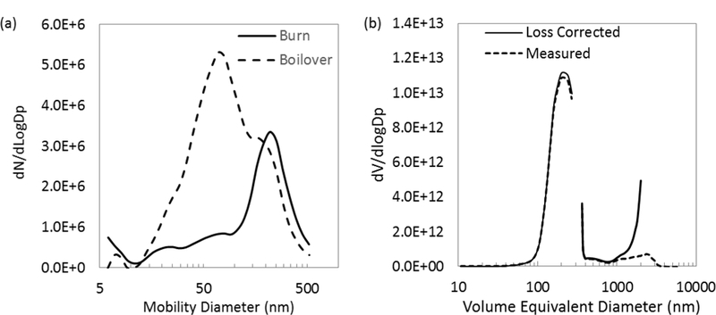
(a) Particle number distributions corrected for sampling losses and background levels, averaged over the first part of the burn and the boilover phases; and (b) burn averaged volume distributions as measured and corrected for sampling line losses.

Oil and Post-Burn Residuals

Analyses were conducted of four samples of crude oil taken from the barrels throughout the testing, a triplicate sample of the oil burn residue from atop the seawater, and three samples of the seawater collected after multiple burns. Results are reported in Table 6.

Table 6.

Organic Analyses (TPH) of Raw Crude Oil, Post-Burn Residuals, and Post-Burn Seawater

	Raw Crude Oil		Post-Burn Residual		Post-Burn Seawater
	mg analyte / g raw oil		mg analyte / g residual oil		mg analyte / L water
	Avg	Std Dev	Avg	Std Dev	Avg	Std Dev
Sum all alkanes	55	3.1	365	36	5.1	5.7
Sum C10-C18 alkanes	34	2.0	120	4.7	1.4	1.6
Sum C19-C27 alkanes	15	0.83	152	9.7	2.3	2.5
Sum C28-C35 alkanes	5.8	0.31	99	26	1.5	1.7
Sum all PAH	14	0.75	90	5.9	1.2	1.4
Sum 2 ring PAH	9.6	0.53	37	1.4	0.45	0.46
Sum 3 ring PAH	4.1	0.19	38	1.4	0.55	0.61
Sum 4 ring PAH	0.59	0.025	8.7	0.35	0.13	0.15
Sum 5+ring PAH	0.030	0.0050	0.54	0.04	0.012	0.013
			Ratios
Total alkanes to PAH	3.8	0.037	4.4	0.32	0.0040	0.0011
AlkaneC10-C18/ alkane C19-C27	2.4	0.013	0.79	0.023	0.00053	0.00023
AlkaneC19-C27/ alkaneC28-C35	2.5	0.051	1.5	0.39	0.0017	0.00019
2 ring PAH / 3 ring PAH	2.3	0.026	1.0	0.0058	0.0010	0.00030
3 ring PAH / 4 ring PAH	7.0	0.063	4.4	0.040	0.0041	0.00026

DISCUSSION

Burn Characteristics and Smoke (PM) Yield

The 19-test average burn rates were 1.30 ± 0.20 mm of oil thickness/min (0.022 ± 0.0033 mm/s) and 2.18 ± 0.37 L oil/min/m². These data compare with reported values of 0.042 mm/s and 2.04 to 2.85 L oil/min/m² [1] and mesoscale tank burns of 0.050 mm/s and 3.5 L oil/min/m² [9], indicating general comparability of our data. The somewhat higher burning rate of the mesoscale data is consistent with data showing that burn rate per unit area increases with fire size [38] and the significantly larger pan size (240 m²) in the mesoscale tank burns as compared to our pan size of 1 m².

Smoke yield, or the PM_ToT emission factor, was 70 ± 8.3 g PM/kg oil_c in our work (Table 7). This value is similar to our value (75 ± 22 g PM/kg oil_c) determined at sea during the Deepwater Horizon in situ burns [5] and much lower than noted for the New Foundland Offshore Burn Experiments (NOBE) burns [7], where yields ranged from 148 to 155 g PM/kg fuel, and mesoscale burns, where yields varied from 94 to 152 g PM/kg fuel [39]. Some research has examined whether fire size affects the smoke yield. Evans et al. [37] measured smoke yield for 40 and 60 cm diameter pool crude oil fires and got 79 g PM/kg oil to 107 g PM/kg oil. Their earlier work indicated smoke yields of 70 to 160 g PM/kg oil as pan diameter was increased from 0.4 m to 7 m. They concluded that smoke yield increased with pan size and that large pool or at sea burns should expect a smoke yield of 150 g PM/kg oil. Koseki and Mulholland [40] showed an increase in smoke yield (mass of PM/kg fuel consumed) over a 10-fold increase in pan area, while our work doubled pan size without a statistically significant effect on PM yield. Field work on three composite Kuwait oil fires (MCE > 98%) [41] report relatively low PM_ToT emission factors (16 to 20 g/kg of fuel consumed), yet individual fires report a wide range of values, from 5 to 52 g/kg of fuel consumed. Undoubtedly, fire size, fuel type, and condition (weathering), as well as environmental conditions, can affect smoke yield. Guenette and Sveum [42] presented some of these factors, specifically slick thickness, the amount of water in the emulsion and the degree of evaporation. Comparison of the PM_2.5 concentrations from our first six sampled burns (average = 69.8 ± 10.0 g PM_2.5/kg oilc) with the nine burns done two days later (average = 49.2 ± 10.3 g PM_2.5/kg oil_c) shows a statistically significant decline in yield (p = 0.0028, α<0.05), possibly due to the additional (18–24 h) air sparging (weathering) for the second day of testing. However, the total petroleum hydrocarbon (TPH) analyses on the raw crude oil over the four day period showed little difference in oil characteristics as seen by the low standard deviation in the Raw Crude Oil column data in Table 6. It should be noted that the TPH analysis does not account for the lightest and most volatile of compounds, which would be expected to exhibit the largest effects of sparging.

Table 7.

Comparison of Emission Factors with Published Results.^a

Compound	Units	This study	References
			[5; 6]	[8]	[2; 3]	[41]g
PM2.5	g/kg oilc	58±14
Total PM	g/kg oilc	70±8.3	75±22	87±15c		48±9%c,f
PCDD/PCDF	ng TEQ/kg oilc	1.2±0.29	1.7
PCDD/PCDF	ng/kg oilc	35±23	74
PAH16 Particle phase	mg/kg oilc	288 ± 83	4.7i
PAH16	mg/kg oilc	980 ± 157
EC	g EC/kg oilc	49±16		66±18		22±27%f
BC	g C/kg	62±12			39, 35b
BC	g BC/kg oilc	53±10
OC	g OC/kg oilc	3.2±1.7		5.2		2.2±27%f
OC	g C/kg oilc			7±3
EC/PM	ratio	0.81±0.08	0.77±0.08’	0.75		0.46±18%f
CO	g CO/kg oilc	58±13		30	54	18
CO	g C/kg oilc	25±5.6		13	23, 27b	7.6±26%f
CO2	g CO2/kg oilc	3,023±21		2,810		2,988
CO2	g C/kg	824±5.7		767±16		815±1%f
CH4	g CO4/kg oilc	1.0±0.45				1.7±44%
CH4	g C/kg	0.75±0.33				1.3±44%
Particles	Particles/kg	5.5±1.3 ×1015			3.9×1015d
MCE	Fraction	0.978±0.004		0.983
VOCs	g/kg oilc	3.4±1.2e		5±6h
MSEE    405 nm	m2/g	10.8±1.4			10.2±4.1
532 nm		9.0±1.2			7.1±2.8

^aBlank - no data. MCE = modified combustion efficiency. MSEE = Mass specific extinction efficiency.

^bAssumes a 90% burn efficiency of oil.

^cPM < 3.5 µm.

^dPM size 0.004–1 µm.

^eSum of U.S. EPA methods TO-15 and TO-11A (88 VOCs).

^fRange of data = relative percent difference.

^gTwo pool fires.

^hSum of 140 different VOCs.

ⁱReference [6].

Some of these distinctions in smoke yield may also be discerned by examining the combustion quality, such as that quantified by the MCE. We observed a 17-run average MCE of 0.978±0.004 which was independent of the doubled pan size or the increased duration of the stored oil weathering through the testing. However, Koseki and Mulholland [40] observed a decrease in MCE from 0.985 to 0.966 when increasing pan size from 0.65 m diameter to 2.4 m diameter. Our MCE value of 0.978 ± 0.004 can be compared with values of 0.94 in Prudhoe crude oil (≤ 60 cm diameter pan) [37] and 0.99 for 1 m and 2.7 m diameter pan sizes with an oil mixture [37]. Aircraft measurements of burning oil showed an MCE value of 0.975 [3]. Tests on a variety of crude oils in a 40 cm diameter water-filled pan [43] found burn efficiencies of 70.3% to 93.8% (average = 84.9%).

Gaseous Carbon Emissions

The emission factors that comprise the MCE, CO at 58 ± 13 g CO/kg oil_c and CO₂ at 3,023 ± 21 g CO₂/kg oil_c, compare well with others’ oil burn data. The literature reports CO values range between 18 and 54 g CO/kg oil [37] as well as 105 g CO/kg oil [37] and CO₂ values of 2,810 [8] and 2,988 [41] g CO₂/kg fuel (Table 7). The at-sea NOBE tests [8] determined 780 ± 16 g C/kg oil which compares with our results at 849 ± 0.3 g C/kg oilc. As for other combustion sources, near road studies of vehicle emissions found a CO emission factor of 31 ± 16 g/kg fuel [44]; studies on prescribed forest fires yielded 116 g CO/kg fuel and CO₂ emission factors of 1,650 g/kg fuel [45].

Particle Size a«d Number Distribution

The PM emitted from the burns exhibited a lognormal distribution (Figure 3a), having a count median mobility diameter of 221 ± 10 nm and a geometric standard deviation of 0.44 ± 0.02. Most of the burns exhibited a second smaller mode around 60 nm. Larger particles (<600 nm) contributed <3% to the total particle concentration. During the thin layer boil over period, the smaller size mode (22 – 80 nm) became more pronounced (Figure 3a). The peak of this smaller size mode was variable, sometimes increasing from ~20 nm up to 80 nm over the duration of the thin layer boilover. In some cases, the larger mode at 220 nm disappeared altogether, and all that remained was this smaller size mode. The optical properties also changed during the thin layer boilover period, as discussed below.

Comparison of particle size distributions across studies is difficult due to the various methods used for particle sizing, which quantify according to different measurements of particle attributes (i.e., mobility diameter, aerodynamic diameter, and volume equivalent diameter). These different measurements are not equivalent for the aggregated particles emitted from oil burns. To overcome these differences, an estimate of the volume distribution (Figure 3b) was made from the mobility distribution measured by the EEPS and the aerodynamic distribution measured by the APS by assuming the effective density and shape factor for methane flame soot [46]. The volume distribution, as measured, exhibits the primary mode with a volume median diameter of 207 ± 9 nm and the indication of a second mode at approximately 2,000 nm. This larger mode was not present during the thin layer boilover period. Correcting for particle losses in the sampling lines suggests that this larger size may have a sizeable contribution to the particle mass. Substantial losses (> 80%) for these larger particles prevent quantification of the mass contained within this larger size mode. However, from the DustTrak PMi size fraction, the fraction of mass in the larger 2,000nm mode is estimated at approximately 20%.

The distributions measured here (volume median diameter 207 nm) are substantially smaller than those measured (volume median diameter 388 nm) in a plume from a DWH in situ burn [3] and the NOBE burns (volume median diameter ~400 nm, [8]). The NOBE burns also exhibited a bimodal distribution with a second peak above 2 µm. Particle concentration emission factors (Table 2) were also approximately 40% larger than the DWH in situ burns [2]. Also, the PM₁ mass fraction here was approximately 80%, which is somewhat larger than other pool fires of varying diameter, including the NOBE burn, which have shown, on average, a PM₁ mass fraction of approximately 65% [37; 39]. Evans et al. [37] found that this fraction decreases with larger diameter pool fires and can increase with aging of the smoke through particle-particle aggregation. Given the sampling conditions and the limitations of comparing across different measurement techniques, our size distributions and mass fractions are consistent with these other reports. We measured fresh emissions, before substantial aggregation could occur, and thus observed higher concentrations of smaller particles than would be observed from larger fires and farther downwind.

Particle Composition

The PM_2.5 mass was composed almost entirely of elemental carbon at 80%, followed by organic carbon at 7%. All inorganic elements (detected by XRF) combined contributed less than 1% to the PM mass. The remaining mass is unidentified but may be due to the O, N, and H atoms associated with the organic carbon or in some cases the metals. This PM composition is comparable to that measured from in situ burns in the Gulf [6]. Other crude oil fires in the laboratory also exhibited elemental carbon fractions between 79 – 86% [37]. The only outlier among the previous oil burns are from the Kuwait fires where only 50% of the PM was elemental carbon. However, the composition of the fuel for these fires was unknown. These crude oil fires exhibit some of the largest elemental carbon fractions observed from any combustion system. At 80% of the PM_2.5 mass, the elemental carbon fraction is larger than kerosene soot (66% [47]), diesel exhaust (51 – 77% [48]), and much larger than gasoline exhaust (12 – 19% [48]) or biomass burning (4.4 – 10.9% [48]).

The elemental carbon emission factor (49 ± 16 g/kg oil_c) is comparable with the 66 ± 18 g/kg fuel from the NOBE tests [8] and the estimated 58 g/kg oilc for the Gulf in situ burns [5; 6] and 39 g/kg oilc black carbon emission factor measured in the Gulf overflights [2]. Black carbon emissions were equivalent to elemental carbon with a black carbon to elemental carbon ratio of 1.08 ± 0.18. These constitute some of the highest known emission factors for black carbon from any source, much greater than controlled combustion sources like on-road diesel engines (0.92 g/kg fuel [49] or gas direct injection engines 0.58 g/kg fuel [44], or open burning sources such as forest fires 0.8–1.5 g/kg fuel [45]. Only kerosene lamps have shown comparable elemental carbon (EC) emission factors at 41 g/kg fuel [47].

Optical Properties

The PM optical properties were approximately constant across all burns. During the thin layer boilover at the end of some burns, the single scattering albedo and absorption angstrom exponent increased as the smoke took on more of a white appearance. The single scattering albedo increased from 0.4 to ~0.6 (at 532 nm), and the absorption angstrom exponent increased from 0.65 to ~0.8 (405 nm - 781 nm). These changes in optical properties may be due to unburned fuel droplets in the emissions during the boilover period as hypothesized by Evans et al. [37]. We suspect that the boilover generates smaller fuel droplets that absorb less light than the larger aggregates generated during oil combustion.

The only other similar measurements for oil burning are from Perring et al. [3], who measured a mass specific extinction efficiency (the amount of light extinction per unit mass concentration of aerosol) of ± 4.1 m²/g at 405 nm (7.1 ± 4.1 m²/g at 532 nm), which is comparable to the 10.8 ± 1.4 m²/g (9.0 ± m²/g) measured here. The mass extinction efficiency is within the range for diesel engine emissions (8.2 ± 0.2 m²/g at 550 nm [50] and kerosene flames (11.1 m²/g at 532 nm [47]. The single scattering albedo of the oil burning emissions was larger (0.40 ± 0.01 at 532 nm) compared to diesel emissions (0.2 ± 0.01 at 550 nm) and kerosene flames (0.26 – 0.43), and the absorption angstrom exponent was much smaller at 0.68 ± 0.03 (405 – 781 nm) than diesel emissions at 1.1 (450 – 700 nm) and kerosene flames at 0.9 (532 – 1047 nm), suggesting that although oil burning particles are composed of mostly EC like these other sources, observed differences in particle morphology or microstructure result in source-specific optical properties. Simulations of aggregate of optical properties have demonstrated that larger primary particle diameters and more compact aggregates can lead to absorption angstrom exponents less than one and larger single scattering albedos [51].

Elemental Composition

The eleven elements shown in Table 4 from the PM_2.5 sampler exceeded the uncertainty level of the measurement by a factor of three. Thirteen samples showed prominent, predictable elements in seawater of Na, Cl, and Si along with S, the latter likely from the oil. However, the majority of the values were below three times the uncertainty and are not reported (see SI Table S18). The NOBE experiments [7] collected PM for metal analysis, with two samplers located on remote control boats and one on an accompanying vessel. Most of the metals (Zn, Fe, Ti, and Ba) were attributed to the composition of the oil boom. However, the average filter weight gain for their trip blank and background samples was similar to the average filter weight gain of the downwind samplers, suggesting minimal capture of the particleladen plume. No other analyses of collected PM appear to have been reported in the literature.

Chemistry by HRTEM

High Resolution Transmission Electron Microscopy (TEM) images are formed by different contributions such as mass, diffraction and phase to the observed contrast [52; 53]. The low magnification bright field image in Figure 4 mainly reflects mass-thickness contrast while the high magnification images revealing the nanostructure rely upon significant phase contrast between directly transmitted and diffracted beams to mark the lattice planes (lamellae) that are evident. The intermediate images are a combination of both contrast mechanisms, though all contribute to varying degrees in any image. In the high angle annular dark field (HAADF) image of Figure 5, the image contrast primarily arises by Rutherford scattering with attendant squared dependence upon atomic number, Z. The relative intensity uniformity in the outer portions of the aggregate is indicative of absence of metals or other high-Z elements. Assuming this to be true for the interior portion of the aggregate, the higher intensity reflects the mass-thickness product of these regions and complements the low magnification bright field image whose intensity similarly reflects the mass thickness.

Figure 4.

Bright field TEM image of the aggregate for Figures 5 and 6.

Figure 5.

An HAADF image of the aggregate shown in Figure 4, as described in the text.

The element-specific images in Figure 6 are formed by STEM mode operation using the 4-segmented EDS detector in the Talos TEM. The focused electron probe provides the spatial specificity with the detectors’ output processed for the particular X-ray energy unique to the specific atom such as carbon or oxygen, as labeled. The particular value is that such images convey the spatial distribution of the particular element with the intensity corresponding to the relative concentration of the element. These images are complementary to the HAADF image where now lighter elements (low-Z atoms) can be effectively spatially mapped by their unique X-ray emission. For carbonaceous soot, carbon is prevalent throughout, as evident by the uniform intensity in the top panel (red) of Figure 6. If oxygen is present, it will be bound to carbon. For such bonded oxygen, the higher imaged concentration will be where there is higher carbon mass - within the aggregate interior. This explanation accounts for the seemingly non-uniform spatial distribution of oxygen (atoms) as TEM images are inherently a 2D projection of a 3-dimensional object. Integrated elemental analysis is consistent with these images where ~ 98 wt% is carbon. Though EDS does not distinguish between matrix bound and surface oxygen, the low O-atom content is likely in the form of surface groups formed during air exposure of the initially hot particles upon release.

Figure 6.

Elemental analysis maps of the aggregate of Figs. 4 and 5 for the color-coded elements. C red, O = green, S = blue.

Volatile Organic Compounds

Benzene was the most abundant VOC in the plume, constituting 51% ± 13% of the 88 VOCs collected. The 10-sample average benzene emission factor was 1,574 ± 372 mg/kg oilc (Table 3). This value corresponds to a benzene content of 0.22% ± 0.05% in the plume, which is similar to the naturally occurring benzene content of the raw crude oil 0.20 wt. % (SI Table S19). Substantially less content in the plume than in the raw oil was found for toluene, ethylbenzene and xylene at 0.027 wt% ± 0.013% vs. 0.53%, 0.0031 wt% ± 0.002% vs. 0.18%, and 0.012 wt % ± 0.009% vs. 0.77%, respectively.

The calculated MCE from each of the collected SUMMA canisters varied between 0.960 and 0.978, implying that the oil burns occurred primarily under incomplete combustion conditions. The emission factors of the classified hazardous air pollutants benzene, acrolein, styrene, 1,3-butadiene, and toluene were found to increase with declining combustion efficiency reflected by decreased MCE (R² = 0.47 to 0.75, SI Figures S2 and S3). Ethylbenzene, o-xylene, m,p-xylene, and formaldehyde had no trends (R² <0.06), while 1,2,4-trimethylbenzene and 1,3,5-trimethylbenzene showed a decrease with increased MCE although these compounds had limited numbers of samples with detectable levels (SI Figure S4). The benzene emission factor (1,574 ± 372 mg/kg oil_c) was notably higher compared to the benzene emission factor computed from traffic 114 ± 38 mg/kg fuel [44] and forest burns 245–776 mg/kg fuel [45].

Formaldehyde was the most abundant carbonyl measured (310 ± 185 mg/kg oil_c), which represented 8% ± 5% of the total VOC emissions during the oil burns. Carbonyl emissions have been minimally reported in the literature for oil burns, and only a few reported carbonyls are comparable with this study. The abundance of formaldehyde, acetaldehyde, acetone, and butyraldehyde was 66%, 15%, 12%, 7% for this study and 20%, 27%, 12%, 41% for the NOBE study [7], respectively. These differences may be due to differences in sampling location, where this study measured carbonyls in the plume directly above the oil burns, and the NOBE study sampled the carbonyls at sea level 50–150 m downwind of the burns.

PCDD/PCDF

The average PCDD/PCDF emission factor, 1.2 ± 1.0 ng TEQ/kg oil_c , was lower than the PCDD/PCDF emission factor measured in the Gulf of Mexico (1.7 ng TEQ/kg oil_c) during the in situ burns [5]. Given the limited sample sizes (n = 4 here and n = 1 in reference [5]), these differences are not notable. Perhaps only two comparable measurements of PCDD/PCDF concentrations have been made during oil fires: one during an experimental at-sea burn similar to those of the Gulf in situ burns [7] and one during mesoscale burns [9] of Louisiana crude when ground-based emission samples were compared against upwind sampling. For the former, results from two samples at sea level were reported as indistinguishable from background levels, leading to the conclusion that PCDDs/PCDFs were not formed from oil spill burns [54; 55]. However, this work was perhaps more concerned with sea-level worker exposure issues as the sampler was on a boat and never sampled the emissions in the lofted plume. Similar conclusions were reached during mesoscale burn tests [9] when the sampler was located at ground level.

Emission measurements in the in situ burn plumes in the Gulf of Mexico [5], analysis of a particle sample from the 2010 Gulf sampling [6], and these current simulations of the 2010 oil burns, confirm that PCDD/PCDF are formed during in situ oil burns. The PCDD/PCDF emission factors for oil burning are comparable to the PCDD/PCDF emission factors for biomass combustion and represent a small portion of the annual U.S. inventory [5; 6]. Homolog profiles, congener patterns, and quality control data are included in the Supporting Information (Tables S-S7, Figures S5-S6).

PAHs

The sum of 16 PAHs results in an emission factor of 980 ± 157 mg PAHs/kg oilc (Table 2) compared with the raw fuel itself at 14.3 ± 0.75 g Total PAHs/kg oil (Table S14). However, the analyses of the raw crude oil for 14 of the 16 EPA PAHs (all but acenaphthylene and anthracene) showed 0.86 ± 0.047 g/kg oil, indicating a near-equivalence between 16-PAH emissions and the original oil content. This observation is contrary to determinations for total PAHs derived elsewhere [54]. We observe the particle- bound PAH₁₆ emissions to be 288 ± 8.3 mg/kg oilc (Table 2) or 0.5% of the PM_2.5 mass, higher than the particle-bound PAH₁₆ emissions observed during Gulf overflights in 2010 [2].

The extractable organic matter fraction of combustion particles shows mutagenic potential that is combustion source dependent. Specifically, the PAH in particle extracts indicate mutagenic potency as measured by the Salmonella assay [56]. Oil burning emits substantial quantities of PAH (see Figure 5 in [6]). In this study, PAH emissions factors measured by GC/MS are given in Table 5 as well as in SI Tables S8-S10. In Table 5, gas and particle-phase combined and particle-phase only PAH emissions factors are given in units of mg/kg of oil consumed, mg B[a]P_eq/kg oil consumed and µg/g of PM. The sixteen EPA- listed priority PAH are the focus but additional particle phase PAH and alkane emission factors are available in SI Tables S9-S10. Individual PAH emission factors (mg/kg oil_c) for the gas- and particle- phase combined vary over approximately two orders of magnitude (2.3 mg/kg oilc - 422 mg/kg oil_c). In total, only 29% w/w of the EPA priority PAH are particle-bound. As expected, results generally show higher gas-phase concentrations of high vapor pressure PAH. For example, naphthalene and acenaphthylene account for more than 50% w/w of the priority PAH emissions. These compounds are classified currently as the intermediate volatility organic compounds (IVOCs) that cause anthropogenic secondary organic aerosol formation, indicating their atmospheric importance.

The EPA priority PAHs account for 0.5% w/w of the particle mass with fluoranthene, phenanthrene, and pyrene explaining the highest proportion of PM (Figure 7). Figure 7 also suggests that the current study produces particles that are among some of the most highly PAH-enriched for oil burning samples. In fact, the results obtained here virtually mimic those produced burning oil in a quartz tube reactor from which sample was collected without dilution [57]. Burning oil in a large-scale calorimeter [37] and in a mesoscale outdoor laboratory [9] similar to the one used here also generated particles enriched in PAH, generally speaking. Gullett et al. [6] implied earlier that laboratory oil burning may not perfectly reflect field conditions, and the present study offers further evidence of this possibility.

Figure 7.

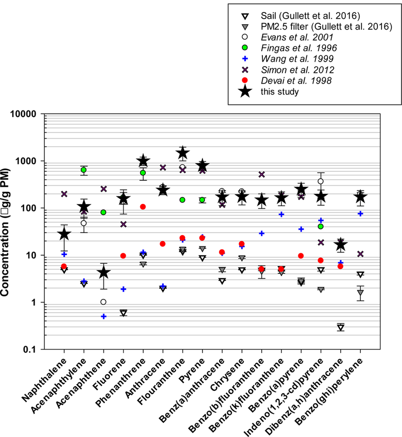
PAH concentrations on PM from burning oil. Data from Gullett et al. (2016) [6], Evans et al. (2001) [37], Fingas et al. (1996) [9], Wang et al. (1999) [58], Simon et al. (2012) [57], Devai et al. (1998) [59].

Residue amounts and characterization

The post-burn, floating oily residue was collected twice daily, each time after multiple burns, for a total of four collections requiring 91 hydrophobic adsorbent pads. The weight gain of the pads, after a negligible amount of water dripped off, amounted to 28.9% by weight of the initial crude oil mass in the residues, indicating only a 71.1% consumption of the oil mass. This consumption value is on the low end of values cited in the literature (90% [60], > 95% [7], 94% [9] and 99% [61]), although no measurement methods or references are provided therein. Volumetric and pressure measurements were used to determine crude oil consumption of 98–99% in mesoscale (2.26 to 13.1 m³) burns [39] and 96 to 98% in mesoscale burns of evaporated (17.4%) and fresh Alaska North Slope crude [37]. Values of 84.9%, somewhat closer to ours, were obtained by Buist et al. [43] with 11 types of crude oil and 84.2% with Light Louisiana Sweet crude oil, emulsified with 0 to 60% water [8]. The type of oil and its state of weathering can have a significant effect on the amount of oil consumed. As well, the water temperature in our work (nominally 6 ^oC) may have affected the comparatively low oil consumption measured.

Data from analysis of the post-burn residuals (Table 6), their weights, and the amount of oil consumed indicate that the alkane content of the residual amounted to over 10% by weight of the oil consumed, 105 ± 3 g alkanes/kg oilc . Similarly, the PAHs in the residuals amount to over 2% of the oil burned, 26 ± 2 g PAHs/kg oilc . The concentration of total PAHs in the residue was 89.65 ± 5.9 mg/g residual oil which is over 100x higher than reported elsewhere at 0.7 mg/g residual oil [9]. This increase may be due to the water temperature and, at least in part, to the cumulative nature of the residuals -- our samples represent a compiled, multi-burn sample whereas the other data [9] appear to represent residuals collected after individual burns.

An analysis of the seawater shows that 13 ± 13 mg alkanes/kg oil burned or approximately 0.0013% of the original oil burned ends up in the water as alkanes (C10-C35). A similar calculation for PAHs suggest ± 3 mg PAHs/kg oil burned or 0.0003% of the oil mass ends up in the water as PAHs.

The post-burn residual oil analysis in comparison with the raw crude analysis is shown in SI Tables SI 14–16. The raw crude oil analysis shows an apparently constant amount of alkanes and PAHs throughout the test program despite constant air sparging of the raw crude barrel. The residual oil shows a factor of six higher alkanes and PAHs mass concentration than the raw crude.

No post-burn residuals were observed on the pan bottoms. The lack of oil burn residues on the pan bottom may be due to the fact that the oil was warm when collected and may sink only after cooling [60].

Our analyses of four post-burn residual oil samples for As, Ba, Cd, Cr, Cu, Pb, Ni, Se, Ag, Na, S, V, Si, and Cl show values above the reporting limit (> 3 × detection limit) for Na and S only. Complete data are listed in the SI Table S17. The NOBE study [7] found little metal in the fresh oil as compared to the weathered oil and residue samples gathered from the boom surface. This observation was believed to be due to metal refractoriness and subsequent concentration in the residue. Of eleven metals analyzed, Mg was 30–100 times that of the next metal, Fe, and over 100 times that of V. None of these metals were notable in our results.

Material Balance

The average amount of oil weight that was lost to combustion products was 71.1% as determined by difference from the weight of collected post-burn residual oil. The weight of all combustion products measured accounted for over 92% of the oil mass lost to combustion. Measurement of H2O was not done and would likely have improved the mass balance. Of the 71.1%, the products were distributed as shown in Figure 8. For example, 2.5% of the original oil mass went to a CO product.

Figure 8.

Fate of combusted oil into products, by weight.

The weight of the combusted oil that went into PMtot was 7.0%. Of this amount, 80% was PM1. Analysis of the PM1 showed that 87% was EC, 7.3% was OC, 0.7% was other elements, and the remaining 5% was unaccounted for.

The post-burn residual oil analysis showed that 28.9% of the initial oil mass was collected as residuals, either in the oil floating on the surface or the oil within the water. Of the floating residue, 36 % was alkanes, 9% was PAHs, and 0.5% was elements, leaving 54% unaccounted.

CONCLUSIONS

Simulations of the at-sea, in situ oil burns during the DWH disaster with Bayou Sweet crude resulted in burn rates and MCE values consistent with past experimental burn data. Smoke yield, or PM emission factors, were generally lower than data gathered from others’ testing with larger burn sizes. The residue mass, 29% of the original crude oil, is on the high end of the literature values, potentially reflecting the cold water temperatures in this study. The PM was fully characterized; virtually all was less than PMi (the count median mobility diameter was 221 ± 10 nm). Over 80% of the PM₁ was EC which is consistent with other source types. However, the single scattering albedo was larger than these sources, suggesting a comparatively lower atmospheric absorption effect. BC values were above all published values for a wide range of source types except for kerosene lamps. Multiple elemental analysis methods of the PM found few remarkable elements (Na, Cl, Si, and S) with the majority, including metals, being below the analytical uncertainty level. Formation of polychlorinated dibenzodioxins/dibenzofurans (PCDDs/DFs) was observed at 1.2 ng toxic equivalency (TEQ)/kg of oil consumed, consistent with past data. VOC measurements showed high benzene emission factors compared to both traffic and forest burn measurements. Particle-bound PAHs amounted to approximately 30% of the total PAH emissions and are among some of the most highly PAH-enriched measurements of oil burn particles. A material balance on the emissions accounted for over 92% of the products, excluding water.

The simulation of the DWH at-sea oil burns resulted in burn characteristics and emission factors that were generally consistent with the literature, allowing our data and the collected particles to be used with confidence in dispersion models, exposure analyses, and toxicology studies to assess the ecological implications of the 2010 Gulf of Mexico burns.

REFERENCES

- 1.Anonymous. Oil Budget Calculator: Deepwater Horizon. . The Federal Interagency Solutions Group, A Report to the Incident Command, US Government, November 2010, http://wwwrestorethegulfgov/sites/default/files/documents/pdf/OilBudgetCalc Full HQ- Print _111110pdf. accessed Feb. 8, 2016.; p 217.; 2010
- 2.Middlebrook AM; Murphy DM; Ahmadov R; Atlas EL; Bahreini R; Blake DR; Brioude J; de Gouw JA; Fehsenfeld FC; Frost GJ; Holloway JS; Lack DA; Langridge JM; Lueb RA; McKeen SA; Meagher JF; Meinardi S; Neuman JA; Nowak JB; Parrish DD; Peischl J; Perring AE; Pollack IB; Roberts JM; Ryerson TB; Schwarz JP; Spackman JR; Warneke C; Ravishankara AR Air quality implications of the Deepwater Horizon oil spill. P Natl Acad Sci USA. 109:20280–20285; 2012 [DOI] [PMC free article] [PubMed] [Google Scholar]
- 3.Perring AE; Schwarz JP; Spackman JR; Bahreini R; de Gouw JA; Gao RS; Holloway JS; Lack DA; Langridge JM; Peischl J; Middlebrook AM; Ryerson TB; Warneke C; Watts LA; Fahey DW Characteristics of black carbon aerosol from a surface oil burn during the Deepwater Horizon oil spill. Geophys Res Lett. 38:5; 2011 [Google Scholar]
- 4.Lane G Air Quality Issues, Air Monitoring Needed for Cleanup Workers in Vessels. Deepwater Horizon Study Group – Working Paper. http://ccrm.berkeley.edu/pdfs papers/DHSGWorkingPapersFeb16- 2011/AirQualityIssuesAirMonitoringNeededForCleanupWorkersinVessels-GL DHSG- Jan2011.pdf; 2011
- 5.Aurell J; Gullett BK Aerostat Sampling of PCDD/PCDF Emissions from the Gulf Oil Spill In Situ Burns. Environ Sci Technol. 44:9431–9437; 2010 [DOI] [PubMed] [Google Scholar]
- 6.Gullett BK; Hays MH; Tabor D; Vander Wal R Characterization of the Particulate Emissions from the BP Deepwater Horizon Spill Surface Oil Burns. Mar Pollut Bull. 107:216–223; 2016 [DOI] [PubMed] [Google Scholar]
- 7.Canada, E. Data Compilation, Newfoundland Offshore Burn Experiment (NOBE) Report. Emergencies Science Division, Environmental Technology Centre, Environment Canada, Ottawa, ON; 1997
- 8.Ross J; Ferek R; Hobbs P Particle and Gas Emissions from an In Situ Burn of Crude Oil on the Ocean. J Air Waste Manag Assoc. 46:251–259; 1996 [DOI] [PubMed] [Google Scholar]
- 9.Fingas M; Li K; Ackerman F; Campagna P; Turpin R; Getty S; Soleki M; Trespalacios M; Wang Z; Paré J; Bélanger J; Bissonnette M; Mullin J; Tennyson E Emissions from mesoscale in situ oil fires: the mobile 1991 experiments. Spill Sci Technol Bull. 3:123–137; 1996 [Google Scholar]
- 10.Lane SM; Smith CR; Mitchell J; Balmer BC; Barry KP; McDonald T; Mori CS; Rosel PE; Rowles TK; Speakman TR; Townsend FI; Tumlin MC; Wells RS; Zolman ES; Schwacke LH Reproductive outcome and survival of common bottlenose dolphins sampled in Barataría Bay, Louisiana, USA, following the Deepwater Horizon oil spill. Proc Biol Sci. 282; 2015 [DOI] [PMC free article] [PubMed] [Google Scholar]
- 11.DeMarini DM; Warren SH; Flen A; Lavrich K; Aurell J; Mitchell W; Greenwell D; Preston W; Hays MD; Samet JM; Gullett BK Mutagenicity and Oxidative Damage Induced by an Organic Extract of the Particulate Emissions from a Simulation of the Deepwater Horizon Surface Oil Burns. Submitted to Environ Mol Mutagen; 2016 [DOI] [PMC free article] [PubMed] [Google Scholar]
- 12.Lyyranen J; Jokiniemi J; Kauppinen EI; Backman U; Vesala H Comparison of different dilution methods for measuring diesel particle emissions. Aerosol Sci Technol. 38:12–23; 2004 [Google Scholar]
- 13.NASA. Alternative Aviation Fuel Experiment. NASA/TM-2011–217059. NASA Langley Research Center, Hampton, VA; 2011 [Google Scholar]
- 14.U.S. EPA Method 10A. Determination of carbon monoxide emissions in certifying continuous emission monitoring systems at petroleum refineries. https://www3.epa.gov/ttnemc01/promgate/m-10a.pdf Accessed July 25, 2016
- 15.U.S. EPA Method 3A. Determination of oxygen and carbon dioxide concentrations in emissions from stationary sources (instrumental analyzer procedure). 1989. http://www.epa.gov/ttn/emc/promgate/m-03a.pdf Accessed May 5, 2014
- 16.40 CFR Part 50, Appendix L. Reference method for the determination of particulate matter as PM2.5 in the Atmosphere. 1987. https://www.gpo.gov/fdsys/pkg/CFR-2014-title40- vol2/pdf/CFR-2014-title40-vol2-part50-appL.pdf Accessed November 22, 2016
- 17.U.S. EPA Compendium Method TO-9A. Determination of polychlorinated, polybrominated and brominated/chlorinated dibenzo-p-dioxins and dibenzofurans in ambient air. 1999. http://www.epa.gov/ttnamti1/files/ambient/airtox/to-9arr.pdf Accessed November 21, 2012
- 18.Hays MD; Smith ND; Kinsey J; Dong YJ; Kariher P Polycyclic aromatic hydrocarbon size distributions in aerosols from appliances of residential wood combustion as determined by direct thermal desorption - GC/MS. J Aerosol Sci. 34:1061–1084; 2003 [Google Scholar]
- 19.Hays MD; Geron CD; Linna KJ; Smith ND; Schauer JJ Speciation of gas-phase and fine particle emissions from burning of foliar fuels. Environ Sci Technol. 36:2281–2295; 2002 [DOI] [PubMed] [Google Scholar]
- 20.U.S. EPA Compendium Method TO-15. Determination of volatile organic compounds (VOCs) in air collected in specially-prepared canisters and analyzed by gas chromatography/mass spectrometry (GC/MS). 1999. http://www.epa.gov/ttnamti1/files/ambient/airtox/to-15r.pdf Accessed November 10, 2015
- 21.U.S. EPA Method 25C. Determination of nonmethane organic compounds (NMOC) in landfill gases. http://www.epa.gov/ttn/emc/promgate/m-25c.pdf Accessed May 11, 2016
- 22.Holder AL; Hagler GSW; Aurell J; Hays MD; Gullett BK Particulate matter and black carbon optical properties and emission factors from prescribed fires in the southeastern United States. J Geophys Res-Atmos. 121:3465–3483; 2016 [Google Scholar]
- 23.Khan B; Hays MD; Geron C; Jetter J Differences in the OC/EC Ratios that Characterize Ambient and Source Aerosols due to Thermal-Optical Analysis. Aerosol Sci Technol. 46:127–137; 2012 [Google Scholar]
- 24.U.S. EPA Compendium Method TO-11A. Determination of Formaldehyde in Ambient Air Using Adsorbent Cartridge Followed by High Performance Liquid Chromatography (HPLC). 1999. https://www3.epa.gov/ttnamti1/files/ambient/airtox/to-11ar.pdf Accessed July 25, 2016
- 25.U.S. EPA Compendium Method IO-3.3. Determination of metals in ambient particulate matter using X-Ray Fluorescence (XRF) Spectroscopy. 1999. http://www.epa.gov/ttnamti1/files/ambient/inorganic/mthd-3-3.pdf Accessed May 5, 2014
- 26.U.S. EPA Method 6010 (SW-846). Inductively Coupled Plasma-Atomic Emission Spectroscopy. 2000. https://www.epa.gov/sites/production/files/2015-07/documents/epa-6010c.pdf Accessed July 25, 2016
- 27.U.S. EPA Method 6020 (SW-846). Inductively Coupled Plasma-Mass Spectroscopy. 1994. https://www.epa.gov/sites/production/files/documents/6020.pdf Accessed July 25, 2016
- 28.U.S. EPA Method 3050B. Acid digestion of sediments, sludges, and soils. 1996. http://www.epa.gov/wastes/hazard/testmethods/sw846/pdfs/3050b.pdf Accessed June 11, 2013
- 29.U.S. EPA Method 8015C (SW-846). Nonhalogenated Organics Using GC/FID 2000. https://www.epa.gov/homeland-security-research/epa-method-8015c-sw-846-nonhalogenated- organics-using-gcfid
- 30.VAnder Wal RBV, ; Hays M Fingerprinting soot (towards source identification): Physical structure and chemical composition. J Aerosol Sci. 41:108–117; 2009 [Google Scholar]
- 31.Rule AM; Geyh AS; Ramos-Bonilla JP; Mihalic JN; Margulies JD Design and characterization of a sequential cyclone system for the collection of bulk particulate matter. J Environ Monitor. 12:1807–1814; 2010 [DOI] [PubMed] [Google Scholar]
- 32.Flowers BA; Dubey MK; Mazzoleni C; Stone EA; Schauer JJ; Kim SW; Yoon SC Optical-chemical-microphysical relationships and closure studies for mixed carbonaceous aerosols observed at Jeju Island; 3-laser photoacoustic spectrometer, particle sizing, and filter analysis. Atmos Chem Phys. 10:10387–10398; 2010 [Google Scholar]
- 33.Virkkula A; Chi X; Ding A; Shen Y; Nie W; Qi X; Zheng L; Huang X; Xie Y; Wang J; Petaja T; Kulmala M On the interpretation of the loading correction of the aethalometer. Atmos Meas Tech. 8:4415–4427; 2015 [Google Scholar]
- 34.U.S. EPA Method 23. Determination of polychlorinated dibenzo-p-dioxins and polychlorinated dibenzofurans from stationary sources. 40 CFR Part 60, Appendix A. 1991. http://www.epa.gov/ttn/emc/promgate/m-23.pdf Accessed November 10, 2015
- 35.Van den Berg M; Birnbaum LS; Denison M; De Vito M; Farland W; Feeley M; Fiedler H; Hakansson H; Hanberg A; Haws L; Rose M; Safe S; Schrenk D; Tohyama C; Tritscher A; Tuomisto J; Tysklind M; Walker N; Peterson RE The 2005 World Health Organization reevaluation of human and mammalian toxic equivalency factors for dioxins and dioxin-like compounds. Toxicol Sci. 93:223–241; 2006 [DOI] [PMC free article] [PubMed] [Google Scholar]
- 36.U.S. EPA Method 8270D (SW-846). Semivolatile Organic Compounds by Gas Chromatography/Mass Spectrometry (GC/MS). 2007. http://www.epa.gov/osw/hazard/testmethods/sw846/pdfs/8270d.pdf Accessed April 24, 2015.
- 37.Evans DMG, Baum H; Walton W; McGrattan K In Situ Burning of Oil Spills. J Res Natl Inst Stan. 106:231–278; 2001 [DOI] [PMC free article] [PubMed] [Google Scholar]
- 38.Evans D, Walton W, Baum H, Mulholland G, Lawson J, Koseki H, & Ghoniem A . Smoke emission from burning crude oil. Artic and Marine Oilspill Program Technical Seminar 1991 [Google Scholar]
- 39.Walton WD; Evans DD; McGrattan KB; Baum HR; Twilley WH; Madrzykowski D; Putorti AD; Rehm RG; Koseki H; Tennyson EJ; Environment, C. In-Situ burning of oil- spills-Mesocale experiments and analysis Proceedings of the Sixteenth Arctic and Marine Oil Spill Program ( Amop ) Technical Seminar, Vols 1 and 2:679–734; 1993 [Google Scholar]
- 40.Koseki H.a.M. G. W The Effect of Diameter on the Burning of Crude Oil Pool Fires. Fire Technol. February 1991:54–65; 1991 [Google Scholar]
- 41.Laursen KK; Ferek R; Hobbs P; Rasmussen RA Emission factors for particles, elemental carbon, and trace gases from the Kuwait oil fires. J Geophys Res. 97:14491–14497; 1992 [Google Scholar]
- 42.Guenette CC; Sveum P In-Situ burning of emulsions R-and-D in Norway. Spill Sci Technol Bull. 2:75–77; 1995 [Google Scholar]
- 43.Buist ITK, ; Morrison J; Aurand D Laboratory studies of the properties of in-situ burn residues. International Oil Spill Conference; 1997 [Google Scholar]
- 44.Zimmerman N; Wang JM; Jeong CH; Ramos M; Hilker N; Healy RM; Sabaliauskas K; Wallace JS; Evans GJ Field Measurements of Gasoline Direct Injection Emission Factors: Spatial and Seasonal Variability. Environ Sci Technol. 50:2035–2043; 2016 [DOI] [PubMed] [Google Scholar]
- 45.Aurell J; Gullett BK Emission Factors from Aerial and Ground Measurements of Field and Laboratory Forest Burns in the Southeastern US: PM2.5, Black and Brown Carbon, VOC, and PCDD/PCDF. Environ Sci Technol. 47:8443–8452; 2013 [DOI] [PubMed] [Google Scholar]
- 46.Tavakoli F; Olfert JS Determination of particle mass, effective density, mass-mobility exponent, and dynamic shape factor using an aerodynamic aerosol classifier and a differential mobility analyzer in tandem. J Aerosol Sci. 75:35–42; 2014 [Google Scholar]
- 47.Chen LWA; Moosmuller H; Arnott WP; Chow JC; Watson JG; Susott RA; Babbitt RE; Wold CE; Lincoln EN; Hao WM Emissions from laboratory combustion of wildland fuels: Emission factors and source profiles. Environ Sci Technol. 41:4317–4325; 2007 [DOI] [PubMed] [Google Scholar]
- 48.Reff A; Bhave PV; Simon H; Pace TG; Pouliot GA; Mobley JD; Houyoux M Emissions Inventory of PM2.5 Trace Elements across the United States. Environ Sci Technol. 43:5790–5796; 2009 [DOI] [PubMed] [Google Scholar]
- 49.Ban-Weiss GA; McLaughlin JP; Harley RA; Lunden MM; Kirchstetter TW; Kean AJ; Strawa AW; Stevenson ED; Kendall GR Long-term changes in emissions of nitrogen oxides and particulate matter from on-road gasoline and diesel vehicles. Atmos Environ. 42:220–232; 2008 [Google Scholar]
- 50.Schnaiter M; Horvath H; Mohler O; Naumann KH; Saathoff H; Schock OW UV-VIS- NIR spectral optical properties of soot and soot-containing aerosols. J Aerosol Sci. 34:1421–1444; 2003 [Google Scholar]
- 51.Scarnato BV; Vahidinia S; Richard DT; Kirchstetter TW Effects of internal mixing and aggregate morphology on optical properties of black carbon using a discrete dipole approximation model. Atmos Chem Phys. 13:5089–5101; 2013 [Google Scholar]
- 52.Lee MR Transmission electron microscopy (TEM) of Earth and planetary materials: A review. Mineralogical Magazine. 74:1–27; 2010 [Google Scholar]
- 53.Midgley PA; Weyland M 3D electron microscopy in the physical sciences: the development of Z-contrast and EFTEM tomography. Ultramicroscopy. 96:413–431; 2003 [DOI] [PubMed] [Google Scholar]
- 54.Fingas MHG, ; Ackerman F; Nelson R; Bissonnette M; Laroche N; Wang Z; Lambert P; Li K; Jokuty P; Sergy G; Tennyson E; Mullin J; Hannon L; Turpin R; Campagna P; Halley W; Latour J; Galarneau R; Ryan B; Aurand D; Hiltabrand R . The Newfoundland offshore burn experiment -NOBE, 1995. . 1995 International Oil Spill Conference Proceedings, Long Beach, CA:123–132; 1995 [Google Scholar]
- 55.Fingas MLP, ; Li K; Wang Z; Ackerman F; Whiticar S; Goldthorp M; Schutz S; Morganti M; Turpin R; Nadeau R; Campagna P; Hiltabrand R . Studies of emissions from oil fires. 1999 International Oil Spill Conference, paper #133; 1999 [Google Scholar]
- 56.Mutlu EWSM, ; Ebersviller SM; Kooter IM; Schmid JE; Dye JA; Linak WP; Gilmour MI; Jetter JJ; Higuchi M; DeMarinie DM . Mutagenicity- and Pollutant-Emission Factors for Solid-fuel Cookstoves: Comparison to Other Combustion Sources. Environ Health Perspect. 124:974–982; 2016 [DOI] [PMC free article] [PubMed] [Google Scholar]
- 57.Simon V; Moreau L; Romdhana MH; Sablayrolles C; Montrejaud-Vignoles M; Lecomte D Emissions of polycyclic aromatic hydrocarbon particulates from combustion of different fuels. Fresenius Environ Bull. 21:946–955; 2012 [Google Scholar]
- 58.Wang Z; Fingas M; Shu YY; Sigouin L; Landriault M; Lambert P; Turpin R; Campagna P; Mullin J Quantitative Characterization of PAHs in Burn Residue and Soot Samples and Differentiation of Pyrogenic PAHs from Petrogenic PAHs-The 1994 Mobile Burn Study. Environ Sci Technol. 33:3100–3109; 1999 [Google Scholar]
- 59.Devai I; DeLaune RD; Henry CB Jr; Lindau CW; Roberts PO Environmental significance of atmospheric emission resulting from In situ burning of oiled salt marsh. Mar Environ Res. 45:157–167; 1998 [Google Scholar]
- 60.Potter SBI, In-situ burning for oil spills in Arctic waters: State-of-the-art and future research needs in: Davidson WFLK, ; and Cogswell A , ed. Oil Spill Response: A global perspective: Springer Science & business Media B.V.; 2008 [Google Scholar]
- 61.Fingas MAF, ; Li K; Lambert P; Wang ZD;; Bissonnette MCC,P; Boileau P; Laroche N;; Jokuty PN,R; Turpin R; Trespalacios M; Halley G;; Belanger JP,J; Vanderkooy N; Tennyson EJ; Aurand D; Hiltabrand R In Proceedings of The 17th Arctic and Marine Oil Spill Program (AMOP) Technical Seminar: Environment Canada: Ottawa, ON,; 1994 [Google Scholar]
Associated Data
This section collects any data citations, data availability statements, or supplementary materials included in this article.