Probe–Sample Interaction-Independent Atomic Force Microscopy–Infrared Spectroscopy: Toward Robust Nanoscale Compositional Mapping

Abstract

Nanoscale topological imaging using atomic force microscopy (AFM) combined with infrared (IR) spectroscopy (AFM-IR) is a rapidly emerging modality to record correlated structural and chemical images. Although the expectation is that the spectral data faithfully represents the underlying chemical composition, the sample mechanical properties affect the recorded data (known as the probe–sample-interaction effect). Although experts in the field are aware of this effect, the contribution is not fully understood. Further, when the sample properties are not well-known or when AFM-IR experiments are conducted by nonexperts, there is a chance that these nonmolecular properties may affect analytical measurements in an uncertain manner. Techniques such as resonance-enhanced imaging and normalization of the IR signal using ratios might improve fidelity of recorded data, but they are not universally effective. Here, we provide a fully analytical model that relates cantilever response to the local sample expansion which opens several avenues. We demonstrate a new method for removing probe–sample-interaction effects in AFM-IR images by measuring the cantilever responsivity using a mechanically induced, out-of-plane sample vibration. This method is then applied to model polymers and mammary epithelial cells to show improvements in sensitivity, accuracy, and repeatability for measuring soft matter when compared to the current state of the art (resonance-enhanced operation). Understanding of the sample-dependent cantilever responsivity is an essential addition to AFM-IR imaging if the identification of chemical features at nanoscale resolutions is to be realized for arbitrary samples.

Atomic force microscopy (AFM) techniques, including photoinduced-force microscopy (PiFM), peak-force infrared microscopy (PFIR), and photothermal-induced resonance (PTIR), have been widely used to detect optical spectroscopic data from absorbing samples.¹⁻⁴ Each technique provides a measure of the local sample absorbance, but other properties that might also contribute to image contrast are not fully understood. In particular, AFM-IR is an imaging modality that uses AFM to measure the PTIR signal produced by a pulsed IR laser^5,6 with theorized resolutions significantly below the diffraction limits of far-field IR microscopy.⁷ In response to an IR laser with a slow repetition rate (∼1 kHz), the approach records data by exciting cantilever oscillation at resonant modes to produce a ringdown signal with an amplitude proportional to the local sample absorbance.^4,8−12 Newer adaptations of this technique operate at higher frequencies and incorporate lock-in detection of the cantilever deflection signal, demonstrating improvements in the signal-to-noise ratio (SNR) and data acquisition speed. The AFM-IR technique has been shown to closely resemble far-field FTIR transmission spectra.^13,14 At present, however, this imaging modality suffers from signal fluctuations resulting from probe–sample mechanical interactions.¹⁵ These fluctuations can have little or no correlation to the local sample expansion (or spectral contrast). It has been shown that these fluctuations can be mitigated by tracking a cantilever-resonance peak¹⁶ during data acquisition (hereafter referred to as resonance-enhanced operation) or by using IR-peak ratios¹⁵ for analysis postacquisition. These methods, however, restrict the available data and are not always effective. Improved optomechanical probes can be designed to be less sensitive to mechanical-property variations.¹⁷ To date, however, imaging sample expansion free of probe–sample mechanical interactions has not been demonstrated.

Resonance-enhanced AFM-IR outperforms scattering-based techniques with greatly improved detection sensitivity¹⁸⁻²¹ and has been successfully demonstrated for thin, weakly absorbing samples across many fields of study.^8,22−25 However, for thick samples at wavelengths corresponding to mid-IR fundamental modes (best for molecular-spectral analysis), absorption is strong and results in a large sample expansion. The sensitivity improvement on resonance is not necessarily realized in these cases, as the laser intensity needs to be reduced (sometimes less than 1% of the full power) to avoid signal saturation or sample melting.²⁶ Moreover, both the amplitude and frequency of resonance peaks are functions of the local mechanical properties of the sample.¹⁶ This results in an undesirable outcome in some cases where the variation in the resonance amplitude becomes dominant, especially for high-frequency resonance modes. As a result, resonance tracking is typically restricted to the low-frequency-cantilever-resonance modes, which have higher levels of noise. Thus, this current-state-of-the-art approach can result in lower sensitivity from the lower-illumination signal and higher noise from operating at lower-resonance modes. The performance ceiling is seemingly limited without an alternate approach. Here, we propose that an explicit analytical understanding of the fundamental imaging process and its dependence on experimental parameters can prevent artifacts in PTIR-signal acquisition and raise the limits of sensitivity and accuracy of AFM-IR imaging. In this report, we first describe the AFM-IR-image-formation process theoretically and then use the insight obtained to develop techniques for improving the accuracy and repeatability of AFM-IR imaging.

Experimental Section

Instrumentation Design and Implementation

The quantum-cascade laser (QCL) and piezo signals were generated using two trigger outputs from a commercially available Nano-IR2 from Anasys Instruments Corporation with a standard Anasys contact-mode probe (PN PR-EX-nIR2-10). The first trigger output was a 100 μs Transistor-Transistor Logic (TTL) pulse that occurred at the start of every trace and retrace scan. Using a National Instruments Data Acquisition (DAQ) device (USB-6009) and lab view, the falling edge of this trigger signal was used to generate two TTL output signals. These output signals switched between high and low voltages at the start of every alternate trace scan, so if one signal was high during the scan, the other signal was low. The second trigger output from the instrument was a TTL pulse train with the repetition rate and pulse width set in the analysis-studio software from Anasys. The two output signals from the DAQ and this trigger signal were fed to a logic circuit to create two TTL pulse-train signals that switched on and off at alternating trace scans. These two signals were fed to the QCL and piezo trigger inputs, respectively, resulting in the desired, interlaced image.

Data Collection and Processing

Measured transfer-function curves were collected using a commercial Nano-IR2 instrument from Anasys Instruments Corporation. The curves were measured by pulsing the QCL laser at a 1 kHz repetition rate with a 300 ns pulse width, averaging the 2048 time-series ringdown profiles, multiplying the time-series ringdown data with a triangle curve, and then applying a Fourier transform. The ringdown measurement was repeated up to 1000 times and averaged in the time domain to further reduce noise for some of the curves shown.

For the equipment used here, the frequency range used for curve fitting was 250 kHz to 2 MHz. Curve fitting was conducted using lsqcurvefit in Matlab with the equations first defined symbolically and then converted to functions using matlabFunction(). We fit an array of n parameters, x(1:n), which had the functional form {m, Γ, ...} = {e^x(1), e^x(1), ...}, in relation to the unknown parameters. This was done to constrain the parameters {m, Γ, ...} to be positive. The desired parameters {m, Γ, ...} and 95% confidence intervals were then determined from the array of fit parameters, x(1:n). The 95% confidence intervals were computed using the outputs from lsqcurvefit as inputs for nlparci functions in Matlab.

A standard protocol was followed for optimally focusing the QCL laser spot to the sample under the AFM tip. The QCL spot position was swept through the area using the Analysis Studio spot-optimization software from Anasys Corporation while pulsing at the third cantilever-resonance mode (∼390 kHz) to reduce the influence of the cantilever heating. This provided sufficient QCL focus optimization for all samples tested in the paper.

All other data and images shown were collected using the operations described in the responsivity-correction-methodology section with the QCL laser-pulse width set to 500 ns and the lock-in time constant set according to the scan rate of the collected data (unless otherwise specified). For example, the polystyrene–polybutadiene–polystyrene polymer images were collected at a 0.5 Hz scan rate (trace and retrace) with 1000 × 1000 pixels, resulting in a lock-in time constant of 1 ms. Resonance tracking was performed using the built-in procedure for the Nano-IR2 with frequency-threshold values of approximately ±20 kHz around the desired resonant frequency. All data sets were collected using nominally identical probes.

Polymer-Test-Sample Preparation

PMMA films were fabricated by spinning 950PMMA A2 photoresist from MicroChem Corporation to 100 nm thickness. The gold mirrors used were economy gold mirrors from Thor Laboratories (PN ME05S-M01), and the silicon wafer was from University Wafers (ID 453). The films were spun at 3000 rpm for 60 s using a headway spinner and then heated to 180 °C for 5 min. The 1951 United States Air Force (USAF) target was fabricated using a Raith Eline (electron-beam-lithography system) at a voltage of 10 kV, a working distance of 10 mm, an area dose of 100 mC/cm², and a line dose of 300 PC/cm to generate the USAF pattern. The targets were then developed in a 1:3 MIBK–IPA solution and heated again above 125 °C to reflow the polymer to produce smooth features.

Polystyrene polybutadiene polymer films were prepared using 0.983 g of a polystyrene–polybutadiene–polystyrene triblock copolymer from Sigma-Aldrich (PN 432490-250G) mixed with 23 mL of toluene and spun at 3000 rpm on a low-emissivity (low-E) slide. Films were scratched to allow for determining the absolute height of the sample and then heated overnight between 60 to 90 °C to allow for phase separation of the two polymers. Overnight, the final film appeared slightly brown and showed phase-separated domains observable using a visible microscope. The phase separation was also apparent when observed using FTIR. The FTIR data is provided in Supplemental Section S4.

Cell Culture and Sample Preparation

MCF 10A (breast epithelial cells) were grown in Dulbecco’s modified Eagle’s medium (DMEM) supplemented with horse serum, hydrocortisone, cholera toxin, epidermal growth factor, insulin, and penicillin–streptomycin. The cells were grown on sterilized low-E glass until 60–70% confluence. Finally, the cells were incubated with a 4% paraformaldehyde solution followed by three PBS washes, quenching with 0.15 M glycine, two PBS washes, and two sterile-water washes. These fixed cells were dried overnight for subsequent imaging.

Results and Discussion

Theoretical Description of the Cantilever-Transfer Function

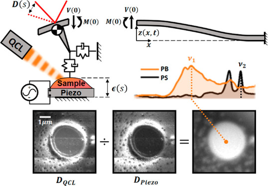
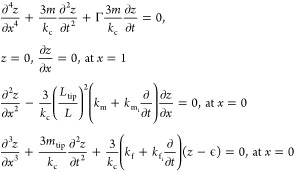
Here, we sought to quantify the dependence of the recorded signal as a function of the actual sample perturbation and the response of the cantilever. The response of a cantilever to an IR-absorbing sample has been studied previously.^4,27 We undertook the development of an analytical model, described in detail in Supplemental Sections S1–S3. A summary of this analysis as well as specific extensions we make for studying nanoscale IR responses are explained below. Considering the free-body diagrams shown in Figure 1a,²⁸ the position of the cantilever can be described as follows:

1

Figure 1.

Transfer-function validation. (a) Free-body diagram of the AFM cantilever beam. The deflection signal (D) is defined as the slope of the cantilever at x_o and is proportional to the sample expansion (ϵ) via the cantilever-transfer function (H_c). (b,c) Transfer-function comparison of the theoretical fit to measured data for a PMMA polymer film and a gold-coated mirror, respectively. (d) Sample-independent curve-fit parameters for the fit data shown in (b,c). (e,f) Sample-dependent fit parameters for the fit data from (b,c).

Equation 1 is a normalized form of Euler–Bernoulli beam theory with a set of boundary conditions specific to this analysis. Here, m is the mass of the cantilever, k_c is the cantilever spring constant, Γ is the viscous dampening of the cantilever, L is the length of the cantilever, L_tip is the length of the cantilever tip, and m_tip is the additional tip mass. The properties that depend on the sample are the expansion signal, ϵ; the lateral spring and damper parameters, k_m and k_mi, and the vertical spring and damper parameters, k_f and k_fi, respectively. These parameters are depicted in Figure 1a.

Our approach is comparable to expressions from previous theories with two major differences: there is additional mass at the tip to account for the tip geometry, and the source that generates the deflection signal is an out-of-plane sample expansion, ϵ, instead of a harmonic point force.^4,27 These additions are both rigorous and necessary for accurately relating the cantilever response to an out-of-plane sample expansion. One relatively straightforward solution to this system is, by means of a transfer function,²⁹ defined by the following:

2

Here, x_o is the position of the deflection laser on the cantilever and H_c(s) is the cantilever-transfer function. The deflection-laser-position parameter, x_o, is depicted in Figure 1a. Equation 2 describes the Laplace domain representation of the input–output response of the cantilever deflection, D(s), to an out-of-plane, free-surface sample-expansion signal, ϵ(s). The expansion signal, ϵ(s), can be considered the expansion of the surface without the presence of the cantilever tip, or a stress-free surface expansion. This follows from concepts in contact mechanics and has been described in previous work.^16,27 Here, we assume the expansion is out-of-plane; however, the deflection signal could theoretically be influenced by lateral sample motion as well. The preferential direction of the motion of the sample is normal to the surface because of the low mechanical impedance of air (i.e., vertical). Special consideration should be taken for samples that are mechanically isolated from neighboring material, such as beads, which would expand isotopically. The vertical-expansion assumption has proven reliable for all samples considered here.

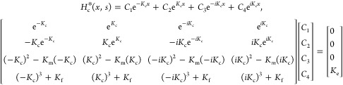
The transfer function from eq 2 can also be considered the cantilever’s responsivity.³⁰ Unlike typical photon detectors, however, the cantilever’s responsivity is influenced by the sample mechanical properties, which mask the desired expansion signal. We propose variations in the cantilever responsivity provide an analytical formulation that explains the previously reported probe–sample-interaction effect. The general solution for the transfer function can be determined by solving the system shown here:

3

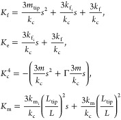
The analytical solution of the transfer function is determined by performing a matrix inversion of eq 3 and then applying the solution to eq 2. For clarity and ease of calculation, the mechanical properties in our formalism have been grouped into four K values. These K values are frequency-dependent stiffness functions that are defined depending on the choice of the tip–sample-stiffness model. For the tip–sample spring-damper model depicted in Figure 1a, the K values are defined here:

4

The four K values shown in eq 4 can be determined by taking the Laplace transform of eq 1. K_c⁴, K_f, K_m, and K_e arise from the resistance to motion of the cantilever, the tip translation, the tip rotation, and the sample motion, respectively. Aspects of the responsivity behavior, such as resonance-frequency shifts, have been demonstrated previously.^4,16 More generally, the definition of the transfer function discussed here reveals all the intricate changes to the cantilever responsivity due to the sample mechanical properties.

Figure 1b,c shows a comparison of the theoretical transfer function and the experimentally measured data using a standard commercial contact-mode probe for a 100 nm poly(methyl methacrylate) (PMMA) polymer film and a gold substrate, respectively. Only frequencies between 250 kHz and 2 MHz were chosen for curve fitting because of noise and discrepancies between the model and the measured data of Figure 1 (see the Experimental Section for details). We believe there is a behavioral change in the cantilever response for low frequencies that is not accounted for by the model; however, for frequencies above 250 kHz, this model provides a theoretical understanding for improving the accuracy of AFM-IR imaging. Possible sources of this behavior are discussed in a later section.

A list of curve-fit values with 95% confidence intervals is provided in Figure 1d–f. Because there are only eight unique parameters, approximate values for k_c, L_tip, and L based on supplier data were used. These three values were assumed to be 0.2 N/m, 10 μm, and 450 μm respectively. All sample-stiffness values show relatively accurate trends, and the added tip mass is about 7% of the total mass of the cantilever. Assuming Hertz contact behavior,³¹ we can approximate the stiffness values as the product of the local effective Youngs modulus and the tip contact-area radius. Assuming a contact radius of 20 nm, the effective Youngs modulus for PMMA and gold are 28 and 65 GPa, respectively. These values are largely dependent on the tip geometry, AFM engagement settings, and film thickness. Regardless, the values presented here are the correct order of magnitude and provide accurate relative values. The mass values equate to a 10 μm radius ball of silicon at the end of a silicon cylindrical beam with a radius of 6 μm and a length of 450 μm. The addition of this tip mass was essential for accurately describing the unique shape of the transfer function. This theory could be adapted to improve the accuracy of measuring the mechanical properties of samples. The idealized spring model from Figure 1a depends on the sample mechanical properties local to the AFM tip (on the order of the tip radius).³² Stiffness measurements of layered samples (like the PMMA film here) would have localized depth dependence and could offer a means to detect surface mechanical properties. For purposes of this paper, the transfer function is used to provide understanding of the responsivity variation present in AFM-IR images.

Cantilever Frequency–Response Investigation

A detailed investigation of the mathematical nature of this transfer function leads to two major conclusions: the deflection signal responds linearly to any out-of-plane sample motion, and the responsivity of the cantilever is dependent on the mechanical properties of the sample local to the cantilever tip. To test the transfer function dependence on the sample mechanical properties, the transfer function was measured by pulsing a quantum cascade laser (QCL) at 1 kHz on both a gold mirror and a 100 nm thick PMMA photoresist film. The resulting ringdown was used to produce the frequency–response curves shown in Figure 2a. These are the same curves from Figure 1b,c, now normalized by the expansion amplitude of PMMA and gold, respectively, to isolate the probe–sample mechanical interaction.

Figure 2.

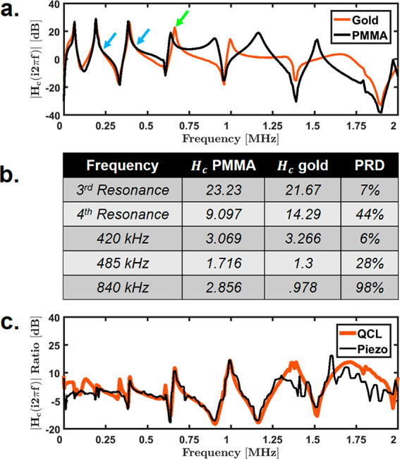
Piezo and QCL frequency responses. (a) Measured transfer functions on 100 nm PMMA film and gold-mirror surface normalized to the scaling factors determined from their respective curve fits in Figure 1. The green arrow indicates a large amplitude change on the fourth resonance mode, and the two blue arrows indicate locations where the transfer functions overlap, suggesting little change in responsivity effect for 225 and 420 kHz. (b) Table of percent relative differences (PRDs) between normalized measured transfer functions on PMMA and gold for ∼390 (third resonance), 420, 485, ∼665 (fourth resonance), and 840 kHz. (c) Ratio of measured gold and PMMA transfer functions using QCL and piezo.

After normalization, the two response curves overlap at the two locations indicated by the blue arrows at ∼225 and ∼420 kHz. This overlap indicates two fixed frequencies that are unaffected by changes in probe–sample mechanical interactions for this setup. It is important to note that these overlap points are specific to the cantilever and instrumentation tested and would vary for different equipment. Interestingly, the amplitudes of the resonance peaks show significant variations between polymer and substrate. An example is the amplitude of the fourth resonance mode (665 kHz), indicated by the green arrow in Figure 2a. In this example, tracking this resonance peak over a heterogeneous sample would produce significant signal fluctuations as a result of the sample mechanical properties. The fifth and sixth cantilever-resonance modes would be entirely impossible to track as they vanish completely upon transition between PMMA and the gold substrate. Because the transfer function is multiplicative, influence of the probe–sample effect can be quantified as the percent relative difference (PRD) between the normalized response curves of any two points P1 and P2 on a given sample, defined as follows:

5

The PRD values for two points located on PMMA and gold for select frequencies are shown in Figure 2b. Low PRD values imply a smaller contribution from the sample mechanical properties in the PTIR signal. The resonance modes do not appear to exhibit any unique isolation from mechanical variations indicated by large PRD values for this sample. In fact, pulsing at fixed 420 kHz appears to be the best candidate for detecting the pure sample expansion signal for the equipment tested here. In general, for an arbitrary sample, measuring the PRD at multiple points could reveal an optimum fixed pulsing frequency for minimizing responsivity effects in AFM-IR images.

The above studies clearly point to the role of cantilever responsivity in both the magnitude and quality of recorded data as well as in the difficulty in conducting resonance-mode experiments. We hypothesize that real-time detection of changes in the cantilever responsivity could greatly improve the fidelity of chemical imaging at nanoscale resolutions. Atomic force acoustic microscopy (AFAM) is one technique that uses out-of-plane vibrations generated by a piezo below the sample for determining the sample mechanical properties.^33,34 Alternative methods exist for determining the mechanical properties of the sample by vibrating the cantilever (known as force-modulation mode);³⁵ however, we propose that out-of-plane sample vibrations more accurately replicate the photoinduced thermal expansion.^36,37 Hence, we hypothesize that measuring the cantilever-response variations in AFM-IR images with a subsample piezo as used in AFAM measurements can provide an accurate measure of the transfer-function variation present in the PTIR signal. To test this idea, the curves in Figure 2a were remeasured using an out-of-plane vibration generated by a piezo actuator placed under the sample. Unlike the curves generated by the QCL alone, the piezo used here has additional acoustic behavior that makes a direct comparison of QCL and piezo signals impossible; however, it is only required that the ratio of the two sample locations have similar frequency responses for proper correction of the responsivity effect. Figure 2c shows the ratio of the measured transfer function on gold and PMMA for both piezo and QCL with good agreement between 250 kHz and 2 MHz. The bandwidth of the piezo used throughout this paper is limited to about 2 MHz; thus, the piezo data becomes increasingly noisy above 1.25 MHz. Additionally, it is currently unclear as to why the behavior deviates for low frequencies. For frequencies above 250 kHz, the piezo-signal response to a stiffness change matches the QCL signal. This data suggests that the piezo signal can be used at fixed frequencies to completely remove cantilever-responsivity variations due to the sample mechanical properties, allowing for an accurate measure of the local sample expansion induced by the absorption of a pulsed infrared laser. Moreover, this technique allows for accurate detection of any thermal-expansion signal and could have potential applications in measuring nanoscale heat transfer as well.^38,39

Responsivity Correction in Nanoscale Chemical Imaging

We modified a commercial nano-IR2 system with the addition of a piezo under the sample. The standard instrument operates by pulsing a QCL while the AFM scans the sample in the standard AFM trace and retrace pattern. The deflection signal is then filtered and fed to a lock-in amplifier to extract the harmonic amplitude of the expansion signal induced by the QCL absorption. The addition of a piezo under the sample allows for the generation of a constant out-of-plane mechanical vibration at the same spatial location and pulsing frequency as the QCL signal to uniquely determine the cantilever responsivity. Real-time detection of two harmonic signals with the same frequency, however, is not possible, so the signals must be separated in either time or frequency space. The best way to do this would be to scan the same line twice, once for the QCL signal and again for the piezo. Another path involves corecording by interlacing the piezo and QCL signals in the same image with a small enough step size to allow for approximate overlap of the two signals. This limits the step size to either the smallest mechanical feature of the sample or the cantilever-tip radius to ensure accurate overlap and requires minimal changes to the commercial instrument. A full description of signal processing is provided in the Experimental Section. Figure 3 shows the four-dimensional data set of interlaced images. After collection, the interlaced lock-in amplitude images can be separated into the two unique data sets and divided to isolate the sample-expansion signal. This is the procedure used for the data presented in this paper. More generally, this process could be extended to measure complex amplitudes of the expansion signal by processing the lock-in phase data as well.

Figure 3.

Responsivity-correction methodology: four-dimensional data set of interlaced QCL and piezo amplitude data showing the cantilever-responsivity-correction operation. The interlaced images are separated into the raw QCL and piezo signals and then divided to produce the corrected images.

Responsivity and IR-Ratio-Correction Methods on Polymer Samples

The responsivity effect produces a multiplicative error that is constant for different wavenumbers but changes with pulsing frequency. As a result, the ratio of recorded absorbance at two wavenumbers postacquisition is a common method for obtaining chemical images.^15,40 The use of two wavenumbers reduces the effectiveness of using a discrete-frequency imaging approach and has increased susceptibility to system drift due to sequential image collection. Hence, we do not recommend the use of this common approach. Moreover, we propose that identifying the contrast of a single wavenumber without responsivity variations is only possible with responsivity-correction techniques. To illustrate the recommendation, we collected PTIR images of a polystyrene polybutadiene polymer film. Figure 4a shows the absolute height image near the edge of the film, and Figure 4b shows the responsivity-corrected 1485 cm^–1 image of the same region. Figure 4c shows point spectra taken at the orange and blue points in Figure 4b. The 1309 and 1485 cm^–1 peaks were selected as characteristic polybutadiene and polystyrene frequencies, respectively, consistent with FTIR-spectroscopy data. Additional details are provided in Supplemental Section S4.

Figure 4.

Responsivity correction on polymer samples. (a) AFM height image flattened and offset relative to the substrate (blue region). Scale bar is 10 μm. Scan rate is 0.5 Hz. (b) Responsivity-corrected PTIR image (1485 cm^–1, 420 kHz) of the same region as that in (a). (c) PTIR point spectra taken at the orange and blue points in (b). (d) Red ROI from (b) showing the raw and responsivity-corrected PTIR images for 1309 and 1485 cm^–1. Blue arrows indicate regions with high responsivity variation resulting from local sample mechanical variations. Scale bar is 1 μm. Scan rate is 1 Hz. (e) Raw piezo signal for each pulsing frequency of the same region as that in (d). (f) Ratio images of 1485 cm^–1 divided by 1309 cm^–1 using the 485 kHz pulsing frequency. The left is the ratio using the raw QCL data, and the right is the ratio using the corrected data.

To avoid aliasing any small features, a 6 μm region was selected and imaged at these wavenumbers for pulsing frequencies 300, 420, and 485 kHz. The pulsing frequencies were chosen to sample the available modulation range: the first harmonic of the laser is limited to 500 kHz, and responsivity correction provides high quality correction above 250 kHz. Moreover, each of these frequencies reveals a significantly different contrast (as a result of their location on the cantilever-transfer-function curve). Figure 4d shows both the raw and responsivity-corrected PTIR images at these pulsing frequencies. The raw images of the beadlike feature for 1309 cm^–1 show enhanced contrast near the interface indicated by the blue arrows in Figure 4d. Without knowledge of the cantilever-responsivity effect, any one of these images would incorrectly suggest a unique chemical feature at the interface of this bead domain. This behavior appears to change with different pulsing frequencies and is equally present in the raw piezo signal also indicated by blue arrows in Figure 4e. After dividing the raw PTIR images with the piezo data, the corrected images for all pulsing frequencies produce comparable contrast, and the interface variation becomes completely absent. This suggests the variation at the interface was the result of contrast due to variations in cantilever responsivity at different pulsing frequencies. This effect is equally present in the 1485 cm^–1 images as well as in most images collected to date using this technique to varying degrees.

Peak ratios have also been used to remove responsivity variations;¹⁵ however, here we show that measuring the responsivity variations in real time ensures reliable IR ratio data. Figure 4f shows 1485–1309 cm^–1 infrared peak-ratio images for a 485 kHz pulsing frequency. The left image is the ratio using the conventionally recorded data, and the right is the ratio using the corrected images proposed here. An inconsistency in the ratio images using current-state-of-the-art methods is shown by the green arrow. This artifact is not present in the ratio data for the other pulsing frequencies using either technique. The wavenumber images were collected 15 min apart, over which time the cantilever response changed slightly as a result of system drift. Redundancies, such as repeated measurements or hyperspectral imaging, could rule out such artifacts, but that reduces the effectiveness of discrete-frequency imaging. Ratio images can be supplemented with local spectra to provide a better understanding in studies. However, the decision to scan the spectrum often relies on a few wavenumber images susceptible to the effects of the sample mechanical properties and their heterogeneity. Here, real-time detection using the piezo signal allowed for proper correction of cantilever-responsivity effects when the ratio method failed.

Responsivity Variations with Resonance-Tracking Techniques

IR chemical imaging of biological samples has been widely attempted with AFM-IR.^8,22,25,41 Resonance-enhanced operation is the current gold standard for minimizing responsivity effects; however, we have found that this is not the case for many samples in biology.¹⁶ Here, we demonstrate improvements in the chemical specificity for AFM-IR imaging compared with the standard resonance-enhanced operation using MCF-10A wild type mammary epithelial cell samples. Figure 5a,b shows the raw PTIR images for a 5 × 5 μm region on a cell sample using fixed 420 kHz and resonance-enhanced operation at the second resonance mode, respectively. The image domain and scan speed here were restricted to ensure accurate tracking for resonance-enhanced operation and sufficient sampling of all sample features. Tracking accuracy was confirmed by comparing the trace and retrace signals for consistency. Further details are provided in Supplemental Figure S4. Comparing the images from Figure 5a,b reveals that operating at different laser-repetition rates can have a significant effect on the contrast because of the dependence on the sample mechanical properties. We have also confirmed that the responsivity-corrected 420 kHz image reveals little change from the raw data, suggesting the difference in contrast shown is due to responsivity effects present in the resonance-tracking image (see Supplemental Figure S4 for responsivity-corrected images). Figure 5c shows the second-resonance-mode peak-frequency image for the same region, which is commonly used to indicate mechanical contrast (resulting from responsivity variations). Here, the resonance-peak frequency and amplitude images show a clear correlation, suggesting a strong influence of responsivity variations in the PTIR signal while tracking the second cantilever-resonance mode. The green, red, and blue boxed regions of Figure 5a–c are enlarged for a clear comparison. Unlike the polymer sample of Figure 4, the PTIR-signal variations here are largely a result of the surface topography and illustrate the challenge of imaging samples that are not prepared with controlled surface characteristics. Tracking a cantilever-resonance mode is insufficient for imaging the pure-sample expansion isolated from responsivity variations for heterogeneous samples.

Figure 5.

Responsivity variations on resonance. (a) PTIR image (1236 cm^–1) of a 5 × 5 μm region of an MCF-10A wild-type mammary epithelial cell using a fixed 420 kHz repetition rate. (b) PTIR image (1236 cm^–1) collected by tracking the second harmonic of the cantilever for the same region as that in (a). (c) Peak-frequency image of the second resonant mode collected simultaneously with (b). Green, red, and blue zoomed sections at the bottom compare the regions of interest indicated in (a–c), respectively. (d) PTIR line profiles for 1525 cm^–1 resonance-tracking operation using the second cantilever-resonance mode with a scan rate of 0.05 Hz. Plot shows one scan and the average of 50 scans for calculating SNR values. (e) Same line profile as in d for the responsivity-corrected 420 kHz fixed-frequency operation for a scan rate of 0.25 Hz. (f) Comparison of scan rates (SRs), signal-to-noise ratios (SNRs), and normalized pixel rates (NPRs) for resonance-enhanced operation (using the second resonance mode) as well as 420 kHz and 485 kHz responsivity-correction operation using the line profiles from (d,e).

In addition to responsivity effects on resonance, we sought to quantify the benefits of the theory and the subsequent approach developed here. Figure 5d shows the PTIR signal of a 5 μm line profile taken at the edge of a breast epithelial cell for 1525 cm^–1 using resonance-enhanced operation at the second resonance mode of the cantilever and a scan rate of 0.05 Hz. The plot shows a representative single scan as well as the average of 50 consecutive scans. Figure 5e shows responsivity-corrected PTIR line profiles for a pulsing frequency of 420 kHz at a scan rate of 0.25 Hz. For equal comparison, the scan rate and lock-in time constant were adjusted such that all the data sets had 1000 samples for every trace scan. Because the resonance-tracking method used requires testing multiple frequencies for locating the resonance peak, the scan rate is 5 times slower when compared with that of a fixed-frequency operation. Figure 5f shows the dark-field-corrected signal-to-noise-ratio (SNR) calculation for each of these profiles. The signal and noise measurements were taken from region 1 of Figure 5d, and the dark-field signal was taken from the substrate section of region 2 for each scan. SNR and scan rates do not provide a good metric for directly comparing imaging techniques. A better way to compare these modalities is via the normalized pixel rate (NPR) defined by⁴²

6

The NPR is proportional to the number of pixels (n) and the well-known scaling between the acquisition time (t) and the resulting SNR for random white noise (SNR ∼ t^1/2). Operating at 420 kHz with responsivity correction is nearly 30 times faster than resonance-enhanced operation using the second resonance mode. Operation at 485 kHz is still faster but only by a factor of ∼5 times compared with that of the resonance-enhanced measurement. This reduction of speed at 485 kHz is due to an increase in responsivity variations combined with the repeatability of the instrument reducing the SNR by a factor of 2. Raw line profiles as well as repeated measurements using smooth samples (SU8 polymer films) are provided in Supplemental Figure S5. Responsivity correction at frequencies with minimal responsivity variations allow for rapid imaging of heterogeneous samples. We emphasize that this demonstration is simply a first example of the implementation of the theoretical insight; better controls and hardware could further improve these figures of merit.

Improving AFM-IR Accuracy and Sensitivity

The sensitivity of resonance-enhanced AFM-IR has been demonstrated previously;¹⁸ here, we apply responsivity correction to demonstrate further improvements in sensitivity and accuracy. Figure 6a shows an AFM height plot of a 1951 USAF resolution target on a silicon wafer fabricated using 100 nm PMMA e-beam photoresist. Resonance-enhanced-operation PTIR line profiles were collected along the magenta line in Figure 6a. Figure 6b shows the PTIR signal for resonance-tracking operation using the first, second, and third cantilever-resonance modes (i–iii, respectively). The magenta- and black-line plots were collected using different QCL laser-focus positions (R1 and R2, respectively). The QCL laser-focus-optimization plots are shown to the right of their respective line profiles. The focus-optimization plots indicate the QCL focus position that produces the highest deflection response. The maximum signal is expected to occur when the laser is optimally focused on the sample under the AFM tip. For the first and second resonance modes, the highest signal in the focus-optimization plots occurs in region R2; however, the PTIR data produced with this laser-focus position shows little contrast. This is true for all three black-line profiles, and most likely suggests that the laser is focused directly to the cantilever beam. Operation using the third resonance mode shows the highest signal with the QCL laser focused to region R1, and the respective magenta-line profile shows reduced noise and improved contrast (resembling the sample height profile) when compared with that of the other two resonance modes. This data suggests the QCL focus position R1 is optimal for maximizing the signal produced by the sample expansion and minimizing the effects of cantilever heating on the recorded data. Moreover, this result demonstrates an increased susceptibility to cantilever heating for the lower cantilever-resonance modes, which is the most likely culprit for the deviation of the measured data and the transfer-function fit observed previously. Top-side QCL illumination, as opposed to the earlier practice of evanescent heating in AFM-IR, will likely heat the cantilever more, which, for very weakly absorbing samples (where sensitivity is crucial), will render the first- and second-harmonic modes less effective. One solution is to operate at higher repetition rates (above the third harmonic, as the data suggests). Figure 6c shows the normalized transfer function on PMMA and silicon for this setup. From lessons learned modeling the cantilever, the presence of the additional mass in the cantilever tip results in large amplitude variations near the fourth (∼610 kHz) and fifth (∼940 kHz) cantilever-resonance modes, making tracking methods virtually impossible in this frequency regime or, at the very least, highly susceptible to the sample mechanical properties. Thus, responsivity correction at fixed frequencies above the third harmonic is one practical solution for avoiding the influence of cantilever heating on recorded data and removing the sample mechanical variations. These factors illustrate the practical challenges in the present state-of-the-art of nanoscale IR measurements and often necessitate careful sample preparation or experimental design by experts. Our proposed approach implements data collection in a manner that will enable this technology to be broadly used by those unfamiliar with the intricate details of potential artifacts.

Figure 6.

Accurate detection of polymer thermal expansion. (a) Height image of group 6 element 4 of 100 nm thick PMMA 1951 USAF target. (b) PTIR-signal line profiles collected at the magenta line in (a). (i–iii) Line profiles for the first-, second-, and third-harmonic resonance-tracking operation, respectively. The frequencies for the first, second, and third resonance modes are approximately 66, 185, and 390 kHz, respectively. The magenta and black plots were taken with the QCL laser focused to regions R1 and R2, respectively. The magenta plot was normalized with its maximum value, and the black-plot mean value was set to 1.5 for clarity. (iv–vi) PTIR-signal intensities with the QCL focus scanned across the sample for first-, second-, and third-harmonics, respectively. Regions R1 and R2 light up because of the focus on the sample and cantilever beam, respectively. The line profiles reveal the most accurate signal when the QCL is focused to region R1 and show decreased noise as the frequency increases. (c) Transfer function for the black and orange points in (a). These plots are normalized according to the procedure shown in Figure 2. Tracking the fifth-harmonic (940 kHz) resonance mode failed because of large variations in peak amplitude. (d) Piezo, QCL, and corrected signal for fixed 940 kHz pulsing frequency at the magenta line in (a). The magenta lines are the actual signals, and the black lines are the predicted signals using only the measured-height profile.

To demonstrate our approach, instead of tracking the fifth resonance peak, we collected profiles using a fixed 940 kHz pulsing frequency and applied responsivity correction. In addition, we illustrate that the signal produced by the subsample piezo represents the local cantilever-responsivity contrast by predicting the raw QCL and piezo profiles using only the silicon and PMMA transfer-function-curve fits and the AFM height profile. Because the laser used here is limited to a 500 kHz repetition rate, we measured the laser second harmonic produced by pulsing at 470 kHz with a 300 ns pulse width. The magenta plots of Figure 6d show raw piezo, raw QCL, and responsivity-corrected line profiles for the magenta line in Figure 6a. Using the curve fits from the transfer functions on PMMA and silicon, we can accurately predict the piezo signal profile; however, the transfer functions only represent two locations on the sample. Because the local sample mechanical properties are dependent on film thickness, we apply a standard correction proposed by Doerner and Nix.³² The predicted piezo signal using the transfer-function-fit data suggests that the measured contrast results from changes in the cantilever responsivity at 940 kHz. The presence of this effect is also apparent in the raw QCL signal. To predict the QCL data, the local sample expansion is also required. The sample chosen for this experiment is sufficiently smooth and thin, which allows for approximating the local sample expansion as a one-dimensional thin-film expansion (i.e., linear with thickness). Thus, the expansion of this sample, to the first approximation, should be proportional to the local thickness of the film with an additional offset to account for substrate heating. Details regarding the one-dimensional-expansion model are provided in Supplemental Section S2.

The measured height data and transfer-function fits allow for predicting the raw piezo and QCL signals. More sophisticated analytical models could be incorporated to better understand the thermal-expansion behavior of samples with well-defined geometries and relate the responsivity-corrected PTIR data to sample expansion. This could provide a heightened understanding of the governing thermoelastic behavior of these materials. For more complex geometry, predicting these signals would require more information and numerical methods for determining the sample expansion. Regardless, this demonstrates that correcting AFM-IR with the signal generated by the piezo enables accurate, model-free detection of the PTIR signal free of responsivity effects. This contrast is theoretically proportional to the desired sample expansion, which more closely resembles the desired spectral information. Additionally, responsivity correction can be performed at any pulsing frequency and is not restricted to low-frequency resonance modes. This allows for lower noise, higher sensitivity, and more accurate imaging than that of resonance-enhanced operation.

Conclusion

Detection of photoinduced thermal expansion with atomic force microscopy (AFM) offers highly sensitive, nanoscale correlated chemical imaging. However, variations in probe–sample mechanical interactions corrupt the underlying chemical contrast. These variations are a direct result of changes in the cantilever response to sample expansion. Here, we developed an analytical understanding of the process and provided practical paths to realizing its advantages. Using a mechanically induced out-of-plane vibration, we show that the responsivity variations can be measured and removed from the AFM-IR signal to isolate the sample expansion. Removing responsivity variations in this way allows for fixed-pulsing-frequency operation, which was shown to improve signal sensitivity by operating outside the noise bandwidth of the system where resonance tracking fails. The methods proposed here demonstrate a more robust chemical-imaging modality with improved accuracy and repeatability when compared with those of the present state-of-the-art (i.e., resonance-enhanced operation). Better piezo controls and hardware as well as higher frequencies offer untapped potential in terms of sensitivity and accuracy, which resonance-enhanced operation alone will never achieve. This work should lead to practical achievements of high-fidelity, robust, lower-noise, and faster nanoscale IR imaging. Moreover, by eliminating the need for detailed knowledge of artifacts and pitfalls to avoid in acquiring accurate data by means of a theoretical understanding, it paves the way for this emerging technique to be widely used by nanoscale researchers with confidence.

Supporting Information Available

The Supporting Information is available free of charge on the ACS Publications website at DOI: 10.1021/acs.analchem.8b00823.

• Supplemental derivation of the cantilever-transfer function, FTIR spectra of test samples, and additional performance data (PDF)

The authors declare no competing financial interest.

References

- Ambrosio A.; Devlin R. C.; Capasso F.; Wilson W. L. Observation of Nanoscale Refractive Index Contrast via Photoinduced Force Microscopy. ACS Photonics 2017, 4 (4), 846–851. 10.1021/acsphotonics.6b00911. [DOI] [Google Scholar]
- Centrone A. Infrared Imaging and Spectroscopy beyond the Diffraction Limit*. Annu. Rev. Anal. Chem. 2015, 8, 101–126. 10.1146/annurev-anchem-071114-040435. [DOI] [PubMed] [Google Scholar]
- Wang L.; Wang H.; Wagner M.; Yan Y.; Jakob D. S.; Xu X. G. Nanoscale simultaneous chemical and mechanical imaging via peak force infrared microscopy. Sci. Adv. 2017, 3 (6), e1700255. 10.1126/sciadv.1700255. [DOI] [PMC free article] [PubMed] [Google Scholar]
- Dazzi A.; Glotin F.; Carminati R. Theory of infrared nanospectroscopy by photothermal induced resonance. J. Appl. Phys. 2010, 107 (12), 124519. 10.1063/1.3429214. [DOI] [Google Scholar]
- Binnig G.; Quate C. F.; Gerber C. Atomic force microscope. Phys. Rev. Lett. 1986, 56 (9), 930–933. 10.1103/PhysRevLett.56.930. [DOI] [PubMed] [Google Scholar]
- Dazzi A.; Prazeres R.; Glotin F.; Ortega J. M. Subwavelength infrared spectromicroscopy using an AFM as a local absorption sensor. Infrared Phys. Technol. 2006, 49 (1–2), 113–121. 10.1016/j.infrared.2006.01.009. [DOI] [Google Scholar]
- Bhargava R. Infrared Spectroscopic Imaging: The Next Generation. Appl. Spectrosc. 2012, 66 (10), 1091–1120. 10.1366/12-06801. [DOI] [PMC free article] [PubMed] [Google Scholar]
- Policar C.; Waern J. B.; Plamont M. A.; Clède S.; Mayet C.; Prazeres R.; Ortega J. M.; Vessières A.; Dazzi A. Subcellular IR imaging of a metal-carbonyl moiety using photothermally induced resonance. Angew. Chem., Int. Ed. 2011, 50 (4), 860–864. 10.1002/anie.201003161. [DOI] [PubMed] [Google Scholar]
- Dazzi A.; Prazeres R.; Glotin F.; Ortega J. M.; Al-Sawaftah M.; de Frutos M. Chemical mapping of the distribution of viruses into infected bacteria with a photothermal method. Ultramicroscopy 2008, 108 (7), 635–641. 10.1016/j.ultramic.2007.10.008. [DOI] [PubMed] [Google Scholar]
- Katzenmeyer A. M.; Aksyuk V.; Centrone A. Nanoscale infrared spectroscopy: Improving the spectral range of the photothermal induced resonance technique. Anal. Chem. 2013, 85 (4), 1972–1979. 10.1021/ac303620y. [DOI] [PubMed] [Google Scholar]
- Katzenmeyer A. M.; Chae J.; Kasica R.; Holland G.; Lahiri B.; Centrone A. Nanoscale Imaging and Spectroscopy of Plasmonic Modes with the PTIR Technique. Adv. Opt. Mater. 2014, 2 (8), 718–722. 10.1002/adom.201400005. [DOI] [Google Scholar]
- Felts J. R.; Kjoller K.; Lo M.; Prater C. B.; King W. P. Nanometer-Scale Infrared Spectroscopy of Heterogeneous Polymer Nanostructures Fabricated by Tip-Based Nanofabrication. ACS Nano 2012, 6 (9), 8015–8021. 10.1021/nn302620f. [DOI] [PubMed] [Google Scholar]
- Ramer G.; Aksyuk V. A.; Centrone A. Quantitative Chemical Analysis at the Nanoscale Using the Photothermal Induced Resonance Technique. Anal. Chem. 2017, 89 (24), 13524–13531. 10.1021/acs.analchem.7b03878. [DOI] [PMC free article] [PubMed] [Google Scholar]
- Hinrichs K.; Shaykhutdinov T. Polarization-Dependent Atomic Force Microscopy–Infrared Spectroscopy (AFM-IR): Infrared Nanopolarimetric Analysis of Structure and Anisotropy of Thin Films and Surfaces. Appl. Spectrosc. 2018, 72 (6), 817–832. 10.1177/0003702818763604. [DOI] [PubMed] [Google Scholar]
- Barlow D. E.; Biffinger J. C.; Cockrell-Zugell A. L.; Lo M.; Kjoller K.; Cook D.; Lee W. K.; Pehrsson P. E.; Crookes-Goodson W. J.; Hung C. S.; Nadeau L. J.; Russell J. N. The importance of correcting for variable probe-sample interactions in AFM-IR spectroscopy: AFM-IR of dried bacteria on a polyurethane film. Analyst 2016, 141 (16), 4848–4854. 10.1039/C6AN00940A. [DOI] [PubMed] [Google Scholar]
- Ramer G.; Reisenbauer F.; Steindl B.; Tomischko W.; Lendl B. Implementation of Resonance Tracking for Assuring Reliability in Resonance Enhanced Photothermal Infrared Spectroscopy and Imaging. Appl. Spectrosc. 2017, 71 (8), 2013–2020. 10.1177/0003702817695290. [DOI] [PubMed] [Google Scholar]
- Chae J.; An S.; Ramer G.; Stavila V.; Holland G.; Yoon Y.; Talin A. A.; Allendorf M.; Aksyuk V. A.; Centrone A. Nanophotonic Atomic Force Microscope Transducers Enable Chemical Composition and Thermal Conductivity Measurements at the Nanoscale. Nano Lett. 2017, 17 (9), 5587–5594. 10.1021/acs.nanolett.7b02404. [DOI] [PMC free article] [PubMed] [Google Scholar]
- Lu F.; Jin M.; Belkin M. A. Tip-enhanced infrared nanospectroscopy via molecular expansion force detection. Nat. Photonics 2014, 8 (4), 307–312. 10.1038/nphoton.2013.373. [DOI] [Google Scholar]
- Huth F.; Govyadinov A.; Amarie S.; Nuansing W.; Keilmann F.; Hillenbrand R. Nano-FTIR absorption spectroscopy of molecular fingerprints at 20 nm spatial resolution. Nano Lett. 2012, 12 (8), 3973–3978. 10.1021/nl301159v. [DOI] [PubMed] [Google Scholar]
- Xu X. G.; Rang M.; Craig I. M.; Raschke M. B. Pushing the sample-size limit of infrared vibrational nanospectroscopy: From monolayer toward single molecule sensitivity. J. Phys. Chem. Lett. 2012, 3 (13), 1836–1841. 10.1021/jz300463d. [DOI] [PubMed] [Google Scholar]
- Ambrosio A.; Jauregui L. A.; Dai S.; Chaudhary K.; Tamagnone M.; Fogler M. M.; Basov D. N.; Capasso F.; Kim P.; Wilson W. L. Mechanical Detection and Imaging of Hyperbolic Phonon Polaritons in Hexagonal Boron Nitride. ACS Nano 2017, 11 (9), 8741–8746. 10.1021/acsnano.7b02323. [DOI] [PubMed] [Google Scholar]
- Giliberti V.; Baldassarre L.; Rosa A.; de Turris V.; Ortolani M.; Calvani P.; Nucara A. Protein clustering in chemically stressed HeLa cells studied by infrared nanospectroscopy. Nanoscale 2016, 8 (40), 17560–17567. 10.1039/C6NR05783G. [DOI] [PubMed] [Google Scholar]
- Kennedy E.; Al-Majmaie R.; Al-Rubeai M.; Zerulla D.; Rice J. H. Quantifying nanoscale biochemical heterogeneity in human epithelial cancer cells using combined AFM and PTIR absorption nanoimaging. Journal of Biophotonics 2015, 8 (1–2), 133–141. 10.1002/jbio.201300138. [DOI] [PubMed] [Google Scholar]
- Khanal D.; Kondyurin A.; Hau H.; Knowles J. C.; Levinson O.; Ramzan I.; Fu D.; Marcott C.; Chrzanowski W. Biospectroscopy of Nanodiamond-Induced Alterations in Conformation of Intra- and Extracellular Proteins: A Nanoscale IR Study. Anal. Chem. 2016, 88 (15), 7530–7538. 10.1021/acs.analchem.6b00665. [DOI] [PubMed] [Google Scholar]
- Baldassarre L.; Giliberti V.; Rosa A.; Ortolani M.; Bonamore A.; Baiocco P.; Kjoller K.; Calvani P.; Nucara A. Mapping the amide I absorption in single bacteria and mammalian cells with resonant infrared nanospectroscopy. Nanotechnology 2016, 27 (7), 075101. 10.1088/0957-4484/27/7/075101. [DOI] [PubMed] [Google Scholar]
- Rosenberger M. R.; Wang M. C.; Xie X.; Rogers J. A.; Nam S. W.; King W. P. Measuring individual carbon nanotubes and single graphene sheets using atomic force microscope infrared spectroscopy. Nanotechnology 2017, 28 (35), 355707. 10.1088/1361-6528/aa7c23. [DOI] [PubMed] [Google Scholar]
- Yuya P. A.; Hurley D. C.; Turner J. A. Contact-resonance atomic force microscopy for viscoelasticity. J. Appl. Phys. 2008, 104 (7), 074916. 10.1063/1.2996259. [DOI] [Google Scholar]
- Bansal R. K.A textbook of strength of materials (in S.I. units), Revised 4th ed.; Laxmi Publications: Bangalore, 2010. [Google Scholar]
- Dorf R. C.; Bishop R. H.. Modern control systems, 9th ed.; Prentice Hall: Upper Saddle River, NJ, 2001. [Google Scholar]
- Razeghi M.Fundamentals of solid state engineering; Kluwer Academic Publishers: Boston, 2002. [Google Scholar]
- Johnson K. L.Contact mechanics; Cambridge University Press: Cambridge, 1985. [Google Scholar]
- Doerner M. F.; Nix W. D. A method for interpreting the data from depth-sensing indentation instruments. J. Mater. Res. 1986, 1 (4), 601–609. 10.1557/JMR.1986.0601. [DOI] [Google Scholar]
- Rabe U.; Amelio S.; Kester E.; Scherer V.; Hirsekorn S.; Arnold W. Quantitative determination of contact stiffness using atomic force acoustic microscopy. Ultrasonics 2000, 38 (1), 430–437. 10.1016/S0041-624X(99)00207-3. [DOI] [PubMed] [Google Scholar]
- Hurley D. C.; Kopycinska-Müller M.; Kos A. B. Mapping mechanical properties on the nanoscale using atomic-force acoustic microscopy. JOM 2007, 59 (1), 23–29. 10.1007/s11837-007-0005-8. [DOI] [Google Scholar]
- Haugstad G.Atomic Force Microscopy: Understanding Basic Modes and Advanced Applications; John Wiley & Sons, Inc.: Hoboken, NJ, 2012. [Google Scholar]
- Rabe U.; Amelio S.; Kopycinska M.; Hirsekorn S.; Kempf M.; Göken M.; Arnold W. Imaging and measurement of local mechanical material properties by atomic force acoustic microscopy. Surf. Interface Anal. 2002, 33 (2), 65–70. 10.1002/sia.1163. [DOI] [Google Scholar]
- Maivald P.; Butt H. J.; Gould S. A. C.; Prater C. B.; Drake B.; Gurley J. A.; Elings V. B.; Hansma P. K. Using force modulation to image surface elasticities with the atomic force microscope. Nanotechnology 1991, 2 (2), 103–106. 10.1088/0957-4484/2/2/004. [DOI] [Google Scholar]
- Heiderhoff R.; Makris A.; Riedl T. Thermal microscopy of electronic materials. Mater. Sci. Semicond. Process. 2016, 43, 163–176. 10.1016/j.mssp.2015.12.014. [DOI] [Google Scholar]
- Collins L.; Ahmadi M.; Wu T.; Hu B.; Kalinin S. V.; Jesse S. Breaking the Time Barrier in Kelvin Probe Force Microscopy: Fast Free Force Reconstruction Using the G-Mode Platform. ACS Nano 2017, 11 (9), 8717–8729. 10.1021/acsnano.7b02114. [DOI] [PubMed] [Google Scholar]
- Van Eerdenbrugh B.; Lo M.; Kjoller K.; Marcott C.; Taylor L. S. Nanoscale mid-infrared evaluation of the miscibility behavior of blends of dextran or maltodextrin with poly(vinylpyrrolidone). Mol. Pharmaceutics 2012, 9 (5), 1459–1469. 10.1021/mp300059z. [DOI] [PubMed] [Google Scholar]
- Dazzi A.; Policar C.. AFM-IR: Photothermal infrared nanospectroscopy: Application to cellular imaging. In Biointerface Characterization by Advanced IR Spectroscopy; Pradier C. M., Chabal Y. J., Eds.; Elsevier: Amsterdam, 2011; pp 245–278. [Google Scholar]
- Bhargava R.; Levin I. W. Spectrochemical Analysis Using Infrared Multichannel Detectors 2007, 1–308. 10.1002/9780470988541.ch1. [DOI] [Google Scholar]
Associated Data
This section collects any data citations, data availability statements, or supplementary materials included in this article.