Bayesian Additive Adaptive Basis Tensor Product Models for Modeling High Dimensional Surfaces: An Application to High-throughput Toxicity Testing.

Summary:

Many modern datasets are sampled with error from complex high-dimensional surfaces. Methods such as tensor product splines or Gaussian processes are effective and well suited for characterizing a surface in two or three dimensions, but they may suffer from difficulties when representing higher dimensional surfaces. Motivated by high throughput toxicity testing where observed dose-response curves are cross sections of a surface defined by a chemical’s structural properties, a model is developed to characterize this surface to predict untested chemicals’ dose-responses. This manuscript proposes a novel approach that models the multidimensional surface as a sum of learned basis functions formed as the tensor product of lower dimensional functions, which are themselves representable by a basis expansion learned from the data. The model is described and a Gibbs sampling algorithm is proposed. The approach is investigated in a simulation study and through data taken from the US EPA’s ToxCast high throughput toxicity testing platform.

1. Introduction

Chemical toxicity testing is vital in determining the public health hazards posed by chemical exposures. However, the number of chemicals far outweighs the resources available to adequately test all chemicals, which leaves knowledge gaps when protecting public health. For example, there are over 80, 000 chemicals in industrial use with fewer than 600 subject to long term in vivo studies conducted by the National Toxicology Program, and most of these studies occur only after significant public exposures.

As an alternative to long term studies, there has been an increased focus on the use of high throughput bioassays to determine the toxicity of a given chemical. To such an end, the US EPA ToxCast chemical prioritization project (Judson et al., 2010) was created to collect dose-response information on thousands of chemicals for hundreds of in vitro bioassays, and it has been used to develop screening methods that prioritize chemicals for study based upon in vitro toxicity. Though these methods have shown utility in predicting toxicity for chemicals that pose a risk to the public health, there are many situations where the in vitro bioassay information may not be available (e.g, a chemical may be so new that it has not been studied). In these cases, it would be ideal if toxicity could be estimated in silico by chemical structural activity relationship (SAR) information. Here the goal is to develop a model based on SAR information that predicts the entire dose-response for a given assay. This manuscript is motivated by this problem.

1.1. Quantitative Structure Activity Relationships

There is a large literature estimating chemical toxicity from SAR information. These approaches, termed Quantitative Structure Activity Relationships (QSAR) (for a recent review of the models and statistical issues encountered see Emmert-Streib et al. (2012)), estimate a chemical’s toxicity from the chemical’s structural properties. Multiple linear regression has played a role in QSAR modeling since its inception (Roy et al., 2015, p. 191), but models where the predictor enters into the model as a linear function often fail to describe the relationship. To address this, approaches such as neural networks (Devillers, 1996), regression trees (Deconinck et al., 2005), support vector machines (Czermiński et al., 2001; Norinder, 2003), and Gaussian processes (Burden, 2001) have been applied to the problem with varying levels of success. These approaches have been tailored to scalar responses, and, save one instance, have not been used to model the dose-response relationship.

The only QSAR approach that has addressed the problem of estimating a dose-response curve is the work by Low-Kam et al. (2015). This approach defined a Bayesian regression tree over functions where the leaves represent a different dose-response surface. It was used to identify chemical properties related to the observed dose-response, and when this approach was applied to prediction the approach sometimes performed poorly in a leave-one-out analysis.

1.2. Relevant Literature

Assume that one obtains a P dimensional vector $s\in \mathcal{S}$, wanting to predict a Q dimensional response over $d\in \mathcal{D}$ from s. Given s (e.g., SAR characteristics in the motivating problem) and d (e.g., doses in the motivating problem) one is interested in estimating an unknown P + Q dimensional surface $h:(\mathcal{S}\times \mathcal{D})\to ℝ$ where response curve i is a cross section of h(s, d) at s_i. Figure 1 describes this in the case of the motivating example; two 1-dimensional cross sections (black lines) of a 2-dimensional surface are observed and one is interested the entire 2-dimensional surface.

Figure 1.

Example of the problem for a 2-dimensional surface. Two 1-dimensional cross sections are observed (black lines) from the larger 2-dimensional surface.

One may use a Gaussian process (GP) (Rasmussen and Williams, 2006) to characterize the entire P + Q dimensional surface, but there are computational problems that make the use of a GP impractical. In the motivating example, there are over 4000 unique (s, d) pairs. GP regression requires inversion of the covariance matrix, which is inherently an $\mathcal{O}(n^3)$ operation; inverting a 4000 × 4000 matrix in each iteration of a Gibbs sampler is challenging. Though the covariance matrix may be approximated leading to reduced computational burden (e.g., Quiñonero-Candela and Rasmussen (2005), Banerjee et al. (2013)), it is the author’s experience that, in the data example, such approximations were accurate when the dimension of the approximation approaches that of the matrix it is approximating. This leads to minimal computational savings. Further, if the approximation approach can be used, the proposed method can be used in conjunction with such approximations.

As an alternative to GPs, one can use tensor product splines (de Boor, 2001, chapter 17), which are frequently based on 1-dimensional spline bases; however, even if one defines a 1-dimensional basis having only two basis functions for each dimension, the resulting tensor spline basis would have dimension 2^P+Q, which is often computationally intractable. The proposed model sidesteps these issues by defining a tensor product of two surfaces defined on $\mathcal{S}$ and $\mathcal{D}$.

Rather than focus on nonparametric surface estimation using GPs or tensor product splines, one could consider the problem from a functional data perspective (Ramsay, 2006; Morris, 2015). As there is interest in the dose response curve defined on $\mathcal{D}$, $\mathcal{S}$ could enter into the model through an additive smooth function; however, if there is an interaction between $\mathcal{D}$ and $\mathcal{S}$ such an approach may not capture the true response surface. To address possible interactions, the functional linear array model (Brockhaus et al., 2015) and functional additive mixed models (Scheipl et al., 2015) allow the surface to be modeled as a basis defined on the entire space. For high dimensional spaces where interactions are appropriate, these approaches only allow the additive terms to depend on one or two dimensions in $\mathcal{S}$, making it difficult to represent higher-order interaction effects.

Clustering the functional responses is also a possibility. Here, one would model the surface using $\mathcal{D}$ and cluster using $\mathcal{S}$. There are many functional clustering approaches (see for example Hall et al. (2001), Ferraty and Vieu (2006), Zhang and Li (2010), Sprechmann and Sapiro (2010), Delaigle and Hall (2013), and references therein), but these methods predict $s\in \mathcal{S}$ based upon observing the functional response f(d), which is the opposite of the problem at hand. In this problem, one observes information on the group (i.e., s), and one wishes to estimate the new response (i.e., h(s, d)). However different, such approaches can be seen as motivating the proposed method. The proposed approach assumes loadings are values on a function defined on $\mathcal{S}$ inducing similarity for any responses having sufficiently close values in $\mathcal{S}$. As loadings are now functions, a new basis is created where each basis function is the tensor product of functions in $\mathcal{S}$ and $\mathcal{D}$.

The proposed approach creates a new basis, and the number of basis functions may impact the model’s ability to represent an arbitrary surface; to model complicated surfaces, a large number of basis functions are included in the model. Parsimony in this set is ensured by adapting to the number of components using the multiplicative gamma prior (Bhattacharya and Dunson, 2011) on the surface loadings. This is a global shrinkage prior that removes components from the sum by stochastically decreasing the prior variance of consecutive loadings to zero. In the manuscript where it was proposed, it was used to overfit the number of factors in a factor analysis; here, it is used to provide an accurate fit.

An alternative way to look at the proposed approach that of an ensemble learner (Sollich and Krogh, 1996), for which there is a vast literature (see Murphy (2012) and references therein). Ensemble learning includes techniques such as bagging (Breiman, 1996) and random forests (Breiman, 2001) and describe the estimate as a weighted sum of learners. The proposed model can be looked at as a weighted sum over tensor product learners.

In what follows, Section 2 defines the model. Section 3 gives the data model for normal responses and outlines a sampling algorithm. Section 4 shows through a simulation study the method outperforms many traditional machine-learning approaches such as treed Gaussian processes (Gramacy and Lee, 2008) and boosted neural networks (Zhou et al., 2002). Section 5 is a data example applying the method to data from the US EPA’s ToxCast database.

2. Model

2.1. Basic Approach

Consider modeling the surface $h:(\mathcal{S}\times \mathcal{D})\to ℝ$ where $\mathcal{S}\subset {ℝ}^P$, P ⩾ 1, and $\mathcal{D}\subset {ℝ}^Q$, Q ⩾ 1. Tensor product spline approaches (de Boor, 2001, chapter 17) approximate h as a product of spline functions defined over $\mathcal{S}$ and $\mathcal{D}$, i.e.,

$$g\otimes f=g(s)f(d),$$

for $g:\mathcal{S}\to ℝ$ and $f:\mathcal{D}\to ℝ$. The tensor product spline defines g and f to be in the span of a spline basis. Assuming g and f are functions in the span of ${\{{\varphi }_j(s)\}}_{j=1}^J$ and ${\{{\nu }_j(d)\}}_{l=1}^L$, that is

$$g(s)=\sum _{j=1}^J{\lambda }_j{\varphi }_j(s),$$

and

$$f(d)=\sum _{l=1}^L{\gamma }_l{\nu }_l(d),$$

the tensor product spline is

$$g\otimes f=\sum _{j=1}^J\sum _{l=1}^L{\rho }_{\mathit{jl}}{\varphi }_j(s){\nu }_l(d),$$

where ρ_jl = λ_jγ_l, and multiple 1-dimensional spline bases are used when P + Q > 2. As this approach typically uses 1- or 2-dimensional spline bases, when the dimension of ($\mathcal{S}$ × $\mathcal{D}$) is large the tensor product becomes impractical as the number of functions in the tensor product increases exponentially.

Where tensor product spline models define the basis a priori, some functional data approaches (e.g, Montagna et al. (2012)) model functions from a basis learned from the data. In these cases, the function space may not be defined over ($\mathcal{S}$ × $\mathcal{D}$), but is constructed on a smaller dimensional subspace ($\mathcal{D}$ in the present discussion). For the cross section at s_i, this approach models h(s_i, d) in the span of a finite basis {f₁(d), …, f_K(d)}. That is,

$$h(s_i,d)=\sum _{k=1}^K{z}_{\mathit{ik}}{f}_k(d),$$ (1)

where (z_i1, …, z_iK)′ is a vector of basis coefficients. This effectively ignores $\mathcal{S}$, which may not be reasonable in many applications.

To model h(s, d) over ($\mathcal{S}$ × $\mathcal{D}$), the functional data and tensor product approaches can be combined. The idea is to define a basis over ($\mathcal{S}$ × $\mathcal{D}$) where each basis function is the tensor product of two surfaces defined on $\mathcal{S}$ and $\mathcal{D}$. Extending (1), define {g₁(s), …, g_K(s)} to be surfaces on $\mathcal{S}$, and replace each z_ik with ζ_kg_k(s_i). Now, loadings are continuous functions on s, and a new basis {g₁ ⊗ f₁, …, g_K ⊗ f_K} is constructed with

$$h(s,d)=\sum _{k=1}^K{\zeta }_k{g}_k(s)\otimes f_k(d).$$ (2)

This model is similar to Brockhaus et al. (2015), but it allows for the dimension of $\mathcal{S}$ to be greater than two and models h(s, d) using multiple tensor products g_k ⊗ f_k.

For the tensor product, the functions ${\{g_k(s)\}}_{k=1}^K$ and ${\{f_k(d)\}}_{k=1}^K$ must be in a linear function space (de Boor, 2001, p. 293). Define

$$g_k~\mathcal{GP}(0,{\sigma }_k^g(\cdot ,\cdot )),$$

and

$$f_k~\mathcal{GP}(0,{\sigma }_k^f(\cdot ,\cdot )),$$

where ${\sigma }_k^g(\cdot ,\cdot )$ and ${\sigma }_k^f(\cdot ,\cdot )$ are positive definite kernel functions. This places g_k and f_k, k = 1, …, K, in a reproducing kernel Hilbert space defined by ${\sigma }_k^g(\cdot ,\cdot )$ or ${\sigma }_k^f(\cdot ,\cdot )$, and embeds h(s, d) in a space defined by the tensor product of these functions.

One may mistake this approach as a GP defined by the tensor product of covariance kernels (e.g., see Bonilla et al. (2007)). That approach forms a kernel over ($\mathcal{S}$ × $\mathcal{D}$) as a product of individual kernels defined on $\mathcal{S}$ and $\mathcal{D}$. For the proposed model, the tensor product is the modeled function and not the individual covariance kernels resulting in a stochastic process that is no longer a GP.

2.2. Selection of K

The value of K determines the number of elements in the basis. The larger K the richer the class of functions the model can entertain. In many cases, one would not expect a large number of functions to contribute and would prefer as few components possible. One could place a prior on K, but it is difficult to find efficient sampling algorithms in this case. As an alternative, the multiplicative gamma process (Bhattacharya and Dunson, 2011) can define a prior over the ζ₁, …, ζ_k that allows the sum to adapt to the necessary number of components. Here,

$${\zeta }_k~N\left(0,{\left[\varphi \prod _{j=1}^k{\delta }_j\right]}^{-1}\right),$$

with ϕ ~ Ga(1, 1) and δ_k ~ Ga(a₁, 1) ⩽ k ⩽ K. This is an adaptive shrinkage prior over the functions. If a₁ > 1, the variances are stochastically decreasing favoring more shrinkage as k increases. For large k, ζ_kg_k(s)f_k(d) nears zero, which implies many of the basis functions contribute negligibly to modeling the surface.

The choice of a₁ defines the level of shrinkage. If a₁ is too large, the model will have too few components contributing to the sum, and if it is too small no shrinkage will take place. In practice, inference from the multiplicative gamma process is robust to choices in a₁, and nearly identical inference was obtained when 1.5 ⩽ a₁ ⩽ 5 for the data example. Following Bhattacharya and Dunson (2011), the choice of a₁ = 2 is reasonable for many applications, and it is used in what follows.

2.3. Relationships to Other Models

Though GPs are used in the model specification, one may use polynomial spline models or process-convolution approaches (Higdon, 2002). Depending on the choice, (2) can degenerate into other methods. For example, if ${\sigma }_1^g,\dots ,g_{K-1}^g$ and ${\sigma }_K^g$ are defined as white noise kernels and f₁(s), ⋯, f_K(s) are in the span of the same basis, the model is identical to the approach of Montagna et al. (2012). In this way, the additive adaptive tensor product model can be looked at as a functional model with loadings correlated by a continuous stochastic process over $\mathcal{S}$.

If the functions g_k and f_k are defined using a spline basis, this approach degenerates to the tensor product spline model. Let each function in {f₁(d), …, f_k(d} be defined using a common basis, with,

$$f_k(d)=\sum _{\ell =1}^L{\beta }_{\ell }{\nu }_{\ell }(d),$$

where ${\{{\nu }_{\ell }(d)\}}_{\ell =1}^L$ is a basis used for all f_k(d). In this case, model (2) can be re-written as

$$h(s,d)=\sum _{k=1}^K\sum _{\ell =1}^L{\zeta }_k{\beta }_{\ell }{g}_k(s){\nu }_{\ell }(d).$$

Letting ${\beta }_{lk}^{\ast }={\zeta }_k{\beta }_{\ell }$, one arrives at a tensor product model with learned basis {g₁(s), …, g_K(s)} defined over $\mathcal{S}$ and specified basis ${\{{\nu }_{\ell }(d)\}}_{\ell =1}^L$ defined over $\mathcal{D}$.

2.4. Computational Benefits

When $\mathcal{D}$ is observed on a fixed number of points and s is the same for each cross section, the proposed approach can deliver substantial reductions in the computational resources needed when compared to GP regression. Let r be the number of unique replicates on $\mathcal{D}$, and let n be the total number of observed cross sections. For a GP, the dimension of the corresponding covariance matrix is rn. Inverting this matrix is an $\mathcal{O}({\left[\mathit{rn}\right]}^3)$ operation. For the proposed approach, there are K inversions of a matrix of dimension r and K inversions of a matrix of dimension n. This results in a computational complexity of $\mathcal{O}(K[r^3+n^3])$, which can be significantly less than a GP based method. In the data example this results in approximately 1/20th the resources needed as compared to the GP approach,(K = 15, n = 669, and r = 7). Savings increase as the experiment becomes more balanced. For example, if n = r and there are the same number of observations as in the data example, then a GP approach would require 10, 000 times more computing time than the proposed method.

3. Data Model

A data model is outlined for normal errors. Extensions to other data generating mechanisms from this framework are straightforward. For example, extensions to count or binomial data are possible using the Pólya – Gamma augmentation scheme of Polson et al. (2013).

For the data model, assume that for cross section i, i = 1, …, n, one observes C_i measurements at ${\{(s_i,d_{\mathit{ic}})\}}_{c=1}^{C_i}$. For error-prone observation y_i(s_i, d_ic), let

$$y_i(s_i,d_{\mathit{ic}})=h(s_i,d_{\mathit{ic}})+{ϵ}_{\mathit{ic}},$$

with ϵ_ic ~ N(0, τ⁻¹). Model (2) assumes the surface is centered at zero; the data model centers it at f₀(d).

In defining h_k(s) and f_k(d), the covariance kernel, along with its hyper-parameters, determines the smoothness of the function. For 1 ⩽ k ⩽ K, let

$${\sigma }_k^g(s,s^{\prime })={\varsigma }_k\exp \left(-{\theta }_k{\parallel s-s^{\prime }\parallel }^2\right),$$ (3)

and

$${\sigma }_k^f(d,d^{\prime })=\exp \left(-{\omega }_k{\parallel d-d^{\prime }\parallel }^2\right),$$ (4)

where ∥·∥ is the Euclidean norm, ς_k is the prior variance, and θ_k and ω_k are scale parameters. For the data model, ζ_k, defined in (2), is not used. Instead it implicitly enters the model through ${\varsigma }_k={(\varphi {\prod }_{j=1}^k{\delta }_j)}^{-1}$. To allow for a variance other than one for f₀, let ${\sigma }_0^f(d,d^{\prime })=\nu \exp (-{\omega }_0{\parallel d-d^{\prime }\parallel }^2)$.

Given these choices, the data model is

$$h(s,d)=f_0(d)+\sum _{k=1}^K{g}_k(s)f_k(d),$$ (5)

and is completely specified by placing priors over ${\{{\sigma }_k^f\}}_{k=0}^K$ and ${\{{\sigma }_k^g\}}_{k=1}^K$. For the length parameter of the squared exponential kernels in (3) and (4), uniform distributions, Unif(a, b), 0 < a < b, are placed over the scale parameters θ_k and ω_k. This places equal prior probability over a range of plausible values allowing the smoothness of the basis to be learned. The value a is chosen large enough so the function is not flat, and b is chosen so that correlation between any two points is approximately 0. These choices are dependent upon the scale of $\mathcal{S}$ and $\mathcal{D}$. Care should be taken in defining b. When b is too large the resultant covariance matrix is essentially a white noise process. It is the author’s experience that this nearly diagonal matrix takes much longer to invert in many linear algebra libraries, increasing computation time. The sampling algorithm used for the data model and corresponding computer code are available in the supplement.

4. Simulation

This approach was tested on synthetic data. The dimension of $\mathcal{S}$ was chosen to be 2 or 3, and for a given dimension, 50 synthetic datasets were created. For each dataset, a total of 1000 cross sections of h(s, d) were observed at seven dose groups. Each dataset contained 7000 observations.

To create a dataset, the chemical information vector s_i, for i = 1, …, 1000, was sampled uniformly over the unit square/cube. At each s_i, h(s_i, d) observations are taken at d = 0, 0.375, 0.75, 1.5, 3.0, 4.5, and 6, from

$$h(s_i,d)=\frac{\nu (s_i)d^m}{\kappa {(s_i)}^m+d^m},$$

where ν(s_i) is the maximum response and κ(s_i) is the dose d where the response is at 50% of the ν(s_i). For all curves, m = 4, and to vary the response over $\mathcal{S}$, a different zero-centered Gaussian process, z(s), was sampled at ${\{s_i\}}_{i=1}^{1000}$, for each simulation, and z(s) is used to define ν(s_i) and κ(s_i) with ν(s_i) = 11 max(z(s_i), 0) and κ(s_i) = max(4.5 − ν(s_i), 0). These choices resulted in the response being between 0 and approximately 50, and ν(s_i) being placed closer to zero for steeper dose-responses. Sample datasets used in the simulation are available in the supplement.

In specifying the model, priors were placed over parameters that reflect assumptions about the curve’s smoothness. For ${\{{\sigma }_k^g(\cdot ,\cdot )\}}_{k=1}^K$, each θ_k was drawn from a discrete uniform distribution over the set {3, 3.05, 3.10, …, 10}. Additionally, for ${\{{\sigma }_k^f(\cdot ,\cdot )\}}_{k=0}^K$, each ω_k ~ Unif(0.1, 1.5). For ${\{{\varsigma }_k\}}_{k=1}^K$, δ_k ~ Ga(2, 1), 1 ⩽ k ⩽ K. The choice of the parameters for the prior over the δ_k were examined. The results were nearly identical with δ_k ~ Ga(5, 1). The prior specification for the model was completed by letting τ ~ Ga(1, 1).

A total of 12000 MCMC samples were taken with the first 2000 disregarded as burn in. For storage purposes, one of ten observations were saved. Trace plots from multiple chains were monitored for convergence, which occurred before 500 iterations.

To analyze the choice of K, the performance of the model was evaluated for K = 1, 2, 3, and 15. The estimates from these models were compared with bagged multivariate adaptive regression splines (MARS) (Friedman, 1991) and bagged neural networks (Zhou et al., 2002) using the ‘caret’ package in R (Kuhn et al., 2016). Additionally, treed Gaussian Processes (Gramacy and Lee, 2008), using the R ‘tgp’ package (Gramacy et al., 2007), were used in the comparison. All packages were run using their default settings; 100 bagged samples were used for both the MARS and neural network models. For the neural network model, 100 hidden layers were used. Posterior predictions from the treed Gaussian process were obtained from the maximum a posteriori (MAP) estimate. This was done as initial tests revealed estimates sampled from the posterior distribution were no better than the MAP estimate, but sampling from the full posterior dramatically increased computation time making the full simulation impossible.

For each dataset, N = 75, 125, and 175 curves were sampled to train the respective model; the remaining curves were compared with predictions using the mean squared predicted error (MSPE).

Table 1 describes the average mean squared predicted error across all simulations. For the adaptive tensor product model there is an improvement in prediction when increasing K. For the 2-dimensional case the improvement occurs from 1 to 2, but the results of K = 3 and 15 are almost identical to K = 2. For the 3-dimensional case, improvements are seen up to K = 3 with identical results for K = 15. This supports the assertion that one can make K large and let the model adapt to the number of tensor products in the sum. When compared with the other approaches, the adaptive tensor product approach is superior. For N = 175, the treed Gaussian process, which is often the closest competitor, produces mean square prediction errors that are about 1.5 times greater than the adaptive tensor product approach. For smaller values of N, the treed GP and the bagged MARS approach failed to produce realistic results in many simulations. Due to this, the 5% trimmed mean provides a better estimate of center.

Table 1.

Mean squared prediction error in the simulation of the adaptive tensor product approach for four values of K as well as treed Gaussian processes, bagged neural networks, and bagged multivariate regression splines (MARS).

		Adaptive TP
		K=1	K=2	K=3	K=15	Neural Net	MARS	Treed GP
2-dimensions	N=75	76.2	69.1	69.5	69.8	108.3	215.21	839.71
	N=125	56.9	48.5	48.8	48.7	92.4	205.8	158.01
	N=175	48.5	37.7	38.4	38.3	85.1	198.8	61.1
3-dimensions	N=75	164.9	162.0	155.4	155.4	185.2	246.61	1521.51
	N=125	128.6	125.0	121.0	121.0	160.4	223.4	421.31
	N=175	106.3	102.6	99.7	100.1	150.0	217.7	163.51

¹Trimmed mean used with 5% of the upper and lower tails removed.

Figure 2, shows where the gains in prediction take place. As a surrogate for the true dose-response function, the response intensity at d = 6 across $\mathcal{S}$ is shown for $\mid \mathcal{S}\mid =2$. Dark gray regions are areas of little-or-no dose-response activity; lighter regions have the steeper dose-responses. Contour plots of the model’s root MSPE are overlaid on the heat maps. The top plot shows the adaptive tensor product performance and the bottom plot shows that of the treed GP, which was the closest competitor for this dataset. The adaptive tensor product is generally better at predicting the dose-response curve across $\mathcal{S}$ and that larger gains are made in regions of high dose response activity.

Figure 2.

Comparison of the predictive performance between the adaptive tensor product and the treed Gaussian process. In the figure, the corresponding model’s root mean squared predicted error is given as a contour plot. The heat map represents the maximum dose response given the coordinate pair; lighter colors represent greater dose-response activity.

To investigate the model’s performance in a situation comparable to the data example, an additional simulation is investigated. Here 50 datasets are constructed where $s\in \mathcal{S}$ are drawn from a 39 dimensional zero centered multivariate normal distribution having an identity covariance. Identically to the above simulation, for each dataset a surface is drawn from a zero centered GP, z(s), with 1000 dose-response curves sampled. In this example, 650 curves are used to train the model with the remaining 350 curves used in a hold out sample. The training of each individual model is more computationally demanding, and the proposed approach is fit using only K = 15 due to the computer resources needed for the full simulation. For comparison, the bagged neural network model using the same configuration above is also fit. Bagged MARS were not considered because the model consistently underperformed the neural network approach in the other simulations. Additionally the treed Gaussian process ware not investigated; initial attempts at training that model failed with either the program failing to complete after 10 hours – implying the entire simulation analyzed using treed GPs would take over 20 days to complete – or crashing. For this simulation, the mean MSPE was 51.1 for the adaptive tensor product method and 58.8 for the bagged Gaussian process, which shows a 12.5% reduction in the MSPE when using the proposed approach.

5. Data Example

The approach is applied to data released from Phase II of the ToxCast high throughput platform. The AttaGene PXR assay was chosen as it has the highest number of active dose-response curves across the chemicals tested. This assay targets the Preganene X receptor, which detects the presence of foreign substances and up regulates proteins involved with detoxification in the body. An increased response for this assay might relate to the relative toxicity of a chemical.

Chemical descriptors were calculated using Mold² (Hong et al., 2008) where chemical structure was described from simplified molecular-input line-entry system (SMILES) information (Weininger, 1988). Mold² computes 777 unique chemical descriptors. For the descriptors, a principal component analysis was performed across all chemicals. This is a standard technique in the QSAR literature (Emmert-Streib et al., 2012, pg 44). Here, the first 38 principal components, representing approximately 95% of the descriptor variability, were used as a surrogate for the chemical descriptor s_i.

The database was restricted to 969 chemicals having SMILES information available. In the assay, each chemical was tested across a range of doses between 0 μM and 250 μM with no tests done at exactly a zero dose. Eight doses were used per chemical, with each chemical tested at different doses. Most chemicals had one observation per dose; however, some of the chemicals tested had multiple observations per dose. In total, the dataset consisted of 9111 data points from the 969 distinct dose-response curves.

A random sample of 669 chemicals was trained to this data, and the remaining 300 observations were used as a hold-out sample. In this analysis, d was the log dose, where this value was rounded to two significant digits. The same prior specification in the simulation was used to train the model, except in the case of the scale parameters ${\{{\theta }_k\}}_{k=1}^K$. As the chemical spaces were defined differently, a discrete uniform prior was placed over the θ_k, which took values in the set {0.05, 0.06, 0.07, …, 3.05}. Here K = 15, and this choice provided identical inference when K = 20 or K = 10. To determine if additional tensor products were necessary the value of ς₁₅ was monitored; it was less than 0.02, indicating additional tensor products were not needed.

To compare the prediction results, boosted MARS and neural networks were used; treed Gaussian processes were attempted, but the R package ‘tgp’ crashed after 8 hours during burn-in. The method of Low-Kam et al. (2015) was also attempted, but, the code was designed such that each chemical is tested at the same doses with the same number of replications per dose point. As the ToxCast data are not in this format, the method could not be applied to the data.

Figures 3 and 4 show the posterior predicted curves (solid black line) with equal tail 90% posterior predicted quantiles (dashed line) for eight chemicals in the hold-out sample. Figure 3 describes the predictions for chemicals having multiple measurements per dose group, and figure 4 gives predictions having only a single observation per dose group. As compared with the observed data, these figures show the model provides accurate dose-response predictions across a variety of shapes and chemical profiles. The grey dashed-dotted line represents the prediction using the bagged neural network. These estimates are frequently less smooth and further o from the observed data than the adaptive tensor product splines. For additional confirmation the model is predicting dose-response curves, one can look a the chemicals from a biological mode of action perspective. For example, in Figure 3, note that the dose-response predictions for both Bisphenol A and 17α Hydroxyprogesterone are similar, because both may act similarly as they are known to bind the estrogen receptor.

Figure 3.

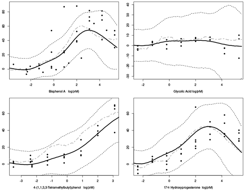
Four posterior predicted dose-response curves (black line) with corresponding 90% equal tail quantiles from the posterior predictive data distribution (dotted lines) for four chemicals in the hold out samples having repeated measurements per dose. Grey dash-dotted line represents the predicted response from the bagged neural network.

Figure 4.

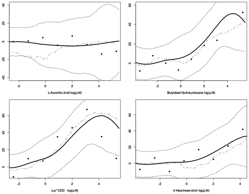
Four posterior predicted dose-response curves (black line) with corresponding 90% equal tail quantiles from the posterior predictive data distribution (dotted lines) for four chemicals in the hold out samples having repeated measurements per dose. Grey dash-dotted line represents the predicted response from the bagged neural network.

In comparison to the other models, the adaptive tensor product approach also had the lowest predicted mean squared error and the predicted mean absolute error for the data in the hold-out sample. Here the model had a predicted mean squared error of 342.1 and mean absolute error of 11.7, as compared with values of 354.7 and 12.4 for neural networks as well as 383.6 and 13.4 for MARS. These results are well in line with the simulation.

One can also compare the ability of the posterior predictive data distribution to predict the observations in the hold out sample. To do this, lower and upper tail cut-points defined by p were estimated from the posterior predictive data distribution. The number of observations below or above the upper cut-point were counted. Assuming the posterior predictive data distribution adequately describes the data, this count is Binomial(2p, n) where n is equal to the number of observations for that chemical. The 90% critical value was computed and compared with the count. This was done for p = 5, 10 and 15%; here, 88, 89, and 90% of the posterior predictive data distributions were at or below the 90% critical value.

6. Conclusions

The proposed approach allows one to model higher dimensional surfaces as a sum of a learned basis, where the effective number of components in the basis adapts to the surface’s complexity. In the simulation and motivating problem, this method is shown to be superior to competing approaches, and, given the design of the experiment, it is shown to require fewer computational resources than GP approaches. Though this approach is demonstrated for high throughput data, it is anticipated it can be used for any multi-dimensional surface.

In terms of the application, this model shows that dose-response curves can be estimated from chemical SAR information, which is a step forward in QSAR modeling. Though such an advance is useful for investigating toxic effects, it can also be used in therapeutic effects. It is conceivable that such an approach can be used in silico to find chemicals that have certain therapeutic effects in certain pathways without eliciting toxic effects in other pathways. Such an approach may be of significant use in drug development as well as chemical toxicity research.

Future research may focus on extending this model to multi-output functional responses. For example, multiple dose-responses may be observed, and, as they target similar pathways, are correlated. In such cases, it may be reasonable to assume their responses are both correlated to each other and related to the secondary input, which is the chemical used in the bioassay. Such an approach may allow for lower level in vitro bioassays, like the ToxCast endpoint studied here, to model higher level in vivo responses.

References

- Banerjee A, Dunson DB, and Tokdar ST (2013). Efficient gaussian process regression for large datasets. Biometrika 100, 75. [DOI] [PMC free article] [PubMed] [Google Scholar]
- Bhattacharya A and Dunson DB (2011). Sparse Bayesian infinite factor models. Biometrika 98, 291–306. [DOI] [PMC free article] [PubMed] [Google Scholar]
- Bonilla EV, Chai KM, and Williams C (2007). Multi-task Gaussian process prediction. In Platt J, Koller D, Singer Y, and Roweiss S, editors, Proc. of the 20th Annual Conference on Neural Information Processing Systems, pages 153–160. Neural Information Processing Systems Conference. [Google Scholar]
- Breiman L (1996). Bagging predictors. Machine Learning 24, 123–140. [Google Scholar]
- Breiman L (2001). Random forests. Machine Learning 45, 5–32. [Google Scholar]
- Brockhaus S, Scheipl F, Hothorn T, and Greven S (2015). The functional linear array model. Statistical Modelling 15, 279–300. [Google Scholar]
- Burden FR (2001). Quantitative structure-activity relationship studies using Gaussian processes. Journal of Chemical Information and Computer Sciences 41, 830–835. [DOI] [PubMed] [Google Scholar]
- Czermiński R, Yasri A, and Hartsough D (2001). Use of support vector machine in pattern classification: Application to QSAR studies. Quantitative Structure-Activity Relationships 20, 227–240. [Google Scholar]
- de Boor C (2001). A practical guide to splines, Revised Edition, volume 27 Springer-Verlag. [Google Scholar]
- Deconinck E, Hancock T, Coomans D, Massart D, and Vander Heyden Y (2005). Classification of drugs in absorption classes using the classification and regression trees (CART) methodology. Journal of Pharmaceutical and Biomedical Analysis 39, 91–103. [DOI] [PubMed] [Google Scholar]
- Delaigle A and Hall P (2013). Classification using censored functional data. Journal of the American Statistical Association 108, 1269–1283. [Google Scholar]
- Devillers J (1996). Neural networks in QSAR and drug design. Academic Press. [Google Scholar]
- Emmert-Streib F, Dehmer M, Varmuza K, and Bonchev D (2012). Statistical modelling of molecular descriptors in QSAR/QSPR. John Wiley & Sons. [Google Scholar]
- Ferraty F and Vieu P (2006). Nonparametric functional data analysis: theory and practice. Springer Science & Business Media. [Google Scholar]
- Friedman JH (1991). Multivariate adaptive regression splines. The Annals of Statistics pages 1–67. [Google Scholar]
- Gramacy RB et al. (2007). tgp: an R package for Bayesian nonstationary, semiparametric nonlinear regression and design by treed Gaussian process models. Journal of Statistical Software 19, 6. [Google Scholar]
- Gramacy RB and Lee HKH (2008). Bayesian treed Gaussian process models with an application to computer modeling. Journal of the American Statistical Association 103, 1119–1130. [Google Scholar]
- Hall P, Poskitt DS, and Presnell B (2001). A functional data-analytic approach to signal discrimination. Technometrics 43, 1–9. [Google Scholar]
- Higdon D (2002). Space and space-time modeling using process convolutions. In Anderson CW, Vic Barnett PC, Chatwin PC, and El-Shaarawi AH, editors, Quantitative methods for current environmental issues, pages 37–54. Springer. [Google Scholar]
- Hong H, Xie Q, Ge W, Qian F, Fang H, Shi L, Su Z, Perkins R, and Tong W (2008). MOLD2, molecular descriptors from 2D structures for chemoinformatics and toxicoinformatics. Journal of Chemical Information and Modeling 48, 1337–1344. [DOI] [PubMed] [Google Scholar]
- Judson RS, Houck KA, Kavlock RJ, Knudsen TB, Martin MT, Mortensen HM, Reif DM, Rotroff DM, Shah I, Richard AM, et al. (2010). In vitro screening of environmental chemicals for targeted testing prioritization: the ToxCast project. Environmental Health Perspectives 118, 485. [DOI] [PMC free article] [PubMed] [Google Scholar]
- Kuhn M, Wing J, Weston S, Williams A, Keefer C, Engelhardt A, Cooper T, Mayer Z, Kenkel B, Benesty M, Lescarbeau R, Ziem A, Scrucca L, Tang Y, Candan C, Hunt T, and the R Core Team. (2016). caret: Classification and regression trainingR package version 6.0-73.
- Low-Kam C, Telesca D, Ji Z, Zhang H, Xia T, Zink JI, Nel AE, et al. (2015). A Bayesian regression tree approach to identify the effect of nanoparticles properties on toxicity profiles. The Annals of Applied Statistics 9, 383–401. [Google Scholar]
- Montagna S, Tokdar ST, Neelon B, and Dunson DB (2012). Bayesian latent factor regression for functional and longitudinal data. Biometrics 68, 1064–1073. [DOI] [PMC free article] [PubMed] [Google Scholar]
- Morris JS (2015). Functional regression. Annual Review of Statistics and Its Application 2, 321–359. [Google Scholar]
- Murphy KP (2012). Machine learning: a probabilistic perspective. MIT press. [Google Scholar]
- Norinder U (2003). Support vector machine models in drug design: applications to drug transport processes and QSAR using simplex optimisations and variable selection. Neurocomputing 55, 337–346. [Google Scholar]
- Polson NG, Scott JG, and Windle J (2013). Bayesian inference for logistic models using Pólya–gamma latent variables. Journal of the American Statistical Association 108, 1339–1349. [Google Scholar]
- Quiñonero-Candela J and Rasmussen CE (2005). A unifying view of sparse approximate Gaussian process regression. Journal of Machine Learning Research 6, 1939–1959. [Google Scholar]
- Ramsay JO (2006). Functional data analysis. Wiley. [Google Scholar]
- Rasmussen CE and Williams CK (2006). Gaussian processes for machine learning. MIT Press. [Google Scholar]
- Roy K, Kar S, and Das RN (2015). Understanding the basics of QSAR for applications in pharmaceutical sciences and risk assessment. Academic Press. [Google Scholar]
- Scheipl F, Staicu A-M, and Greven S (2015). Functional additive mixed models. Journal of Computational and Graphical Statistics 24, 477–501. [DOI] [PMC free article] [PubMed] [Google Scholar]
- Sollich P and Krogh A (1996). Learning with ensembles: How overfitting can be useful. Advances in Neural Information Processing Systems pages 190–196. [Google Scholar]
- Sprechmann P and Sapiro G (2010). Dictionary learning and sparse coding for unsupervised clustering. In 2010 IEEE International Conference on Acoustics Speech and Signal Processing (ICASSP), pages 2042–2045. IEEE. [Google Scholar]
- Weininger D (1988). SMILES, a chemical language and information system: 1. Introduction to methodology and encoding rules. Journal of Chemical Information and Computer Sciences 28, 31–36. [Google Scholar]
- Zhang Q and Li B (2010). Discriminative K-SVD for dictionary learning in face recognition. In 2010 IEEE Conference on Computer Vision and Pattern Recognition (CVPR), pages 2691–2698. IEEE. [Google Scholar]
- Zhou Z-H, Wu J, and Tang W (2002). Ensembling neural networks: many could be better than all. Artificial Intelligence 137, 239–263. [Google Scholar]
Associated Data
This section collects any data citations, data availability statements, or supplementary materials included in this article.