Model-Based Clustering With Data Correction For Removing Artifacts In Gene Expression Data

Abstract

The NIH Library of Integrated Network-based Cellular Signatures (LINCS) contains gene expression data from over a million experiments, using Luminex Bead technology. Only 500 colors are used to measure the expression levels of the 1,000 landmark genes measured, and the data for the resulting pairs of genes are deconvolved. The raw data are sometimes inadequate for reliable deconvolution, leading to artifacts in the final processed data. These include the expression levels of paired genes being flipped or given the same value, and clusters of values that are not at the true expression level. We propose a new method called model-based clustering with data correction (MCDC) that is able to identify and correct these three kinds of artifacts simultaneously. We show that MCDC improves the resulting gene expression data in terms of agreement with external baselines, as well as improving results from subsequent analysis.

1. Introduction

Recent improvements in gene expression measurement technologies, including microarrays (Schena et al., 1995; Lockhart et al., 1996; Ball et al., 2002) and RNAseq (Wang et al., 2009), have greatly increased the amount of data available for analysis. These data offer many opportunities to further biologists' understanding of how cells act in different settings. However, the ability to learn from any method is limited by the quality of the data being used. The quality of data from gene expression experiments is limited by a number of factors, from variability in environmental conditions to uncertainties inherent in the measurement technologies themselves (Liu and Rattray, 2010). The data used for inference have usually gone through a preprocessing pipeline to adjust the data to be more amenable to analysis (Sebastiani et al., 2003). Examples of preprocessing steps include logarithmic transformation of raw fluorescence values and quantile normalization. Although these techniques are often helpful, they can sometimes introduce artifacts into the data (Blocker and Meng, 2013; Lehmann et al., 2013). It is important to identify these additional sources of variation and correct them if possible, or if not, to account for them in the assessment of variability and uncertainty.

Our work is motivated by a gene expression dataset from the NIH Library of Integrated Network-based Cellular Signatures (LINCS) program. One of the aims of the LINCS project is to measure gene expression changes in response to drug and genetic perturbations. In these experiments, cell lines (or cell cultures that can be manipulated in the laboratory) were subjected to different perturbation experiments, in which drugs were applied or genetic makeup was changed. Over 1.4 million experiments have been performed and the expression levels of approximately 1000 genes were measured. Genes were paired in the experimental setup and this led to multiple issues in the processed data, including clustering, switched expression values of the two genes, and assignment of the same expression value to the two genes. We develop a new method to address these issues. The method is an extension of model-based clustering that explicitly incorporates the expression level swaps while simultaneously addressing the other problems in the data. We call it model-based clustering with data correction, or MCDC. We show that our method works well on simulated datasets, and that it improves the gene expression data, both in terms of agreement with an external baseline and in subsequent inference.

Section 2 describes the motivating data for our method. Section 3 outlines our method, MCDC, as well as a practical EM algorithm for implementation. In Section 4 we present a simulation study, showing that our method is able to identify and correct points which have been altered. Section 5 shows how MCDC can be applied to our motivating data to improve the data overall as well as improve subsequent analyses. Section 6 concludes with a discussion.

2. Data

The Library of Integrated Network-based Cellular Signatures (LINCS) program, http://lincsproject.org, is funded by the Big Data to Knowledge (BD2K) Initiative at the National Institutes of Health (NIH) whose aim is to generate genetic and molecular signatures off human cells in response to various perturbations. This program includes gene expression, protein-protein interaction, and cellular imaging data (Vempati et al., 2014). Vidović et al. (2013) used the LINCS data to understand drug action at the systems level, while Shao et al. (2013) used them to study kinase inhibitor induced pathway signatures, and Chen et al. (2015) and Liu et al. (2015) examined the association of chemical compounds with gene expression profile. The LINCS L1000 data has also been combined with chemical structure data to predict adverse drug reactions (Wang et al., 2016).

The LINCS L1000 data is a vast library of gene expression profiles that include over one million experiments covering more than seventy human cell lines. These cell lines are populations of cells descended from an original source cell and having the same genetic makeup, kept alive by growing them in a culture separate from their original source. The L1000 data include experiments using over 20,000 chemical perturbagens, namely drugs added to the cell culture to induce changes in the gene expression profile. In addition, there are genetic perturbation experiments targeting a single gene to control its expression level, either suppressing it (knockdown) or enhancing it (overexpression). The LINCS L1000 data is publicly available for download from http://lincscloud.org and from the Gene Expression Omnibus (GEO) database with accession number GSE70138 http://www.ncbi.nlm.nih.gov/geo/query/acc.cgi?acc=GSE70138. Duan et al. (2014) provide a web application to allow researchers to explore the LINCS L1000 data interactively at http://www.maayanlab.net/LINCS/LCB/.

2.1. Experimental design of the L1000 data

Each individual L1000 experiment measures the expression levels of approximately 1,000 landmark genes in the human genome. The goal of the LINCS project is to capture the cells' response to perturbations. Therefore, the project was designed to include a very large number of experiments, but this came at the cost of measuring only a limited number of selected landmark genes. These landmark genes were selected to cover as much of the variation in cellular gene expression as possible. In each experiment, the selected perturbation was applied and the cells were allowed to culture for a specified period of time before the gene expression levels were measured.

The L1000 experiments were carried out using the Luminex Bead technology (Peck et al., 2006; Dunbar, 2006), in which color-coded microspheres are produced to attach to specific RNA sequences corresponding to a landmark gene and to fluoresce according to the amount of RNA produced as that gene is expressed. To perform a single experiment, a perturbing agent such as a chemical compound is added to the solution. Additionally, around 100 beads are added for each gene to be measured. The beads for measuring a particular gene share a color that can be uniquely identified using lasers. To process an experiment, the beads in the solution are sampled and analyzed to determine which gene they are measuring. Additionally, their fluorescence level is measured to determine the expression level of the gene. With many beads per gene, a good estimate of the overall expression level is obtained.

The L1000 experiments used only 500 bead colors to measure the expression levels of the 1,000 landmark genes. This means that each bead color had to do double duty, accounting for a pair of genes. Thus, when an experiment is processed, a given bead color will have some observations from one gene and the rest from another gene. These gene pairs were selected to have different levels of expression, and the beads for a pair were mixed in approximately a two to one ratio. This means that, ideally, when the beads are sampled, a histogram of fluorescence levels corresponding to gene expression is created with two peaks, one of which has twice the number of observations as the second peak.

2.2. L1000 Data Preprocessing

In order to facilitate statistical analysis of the L1000 data, the raw bead fluorescence measurements were combined and transformed. First, the measurements from many beads of the same color were deconvolved to assign expression values to the appropriate pair of genes. The data then went through multiple normalization steps (Liu et al., 2015; Bolstad et al., 2003). First, a set of genes were identified as being stable across cell lines and perturbations, and these were used to inform a power law transformation of all gene values. The expression values were then quantile-normalized across sets of experiments to make the distribution of expression levels the same for all experiments. These steps are illustrated in Figure 1.

Fig 1.

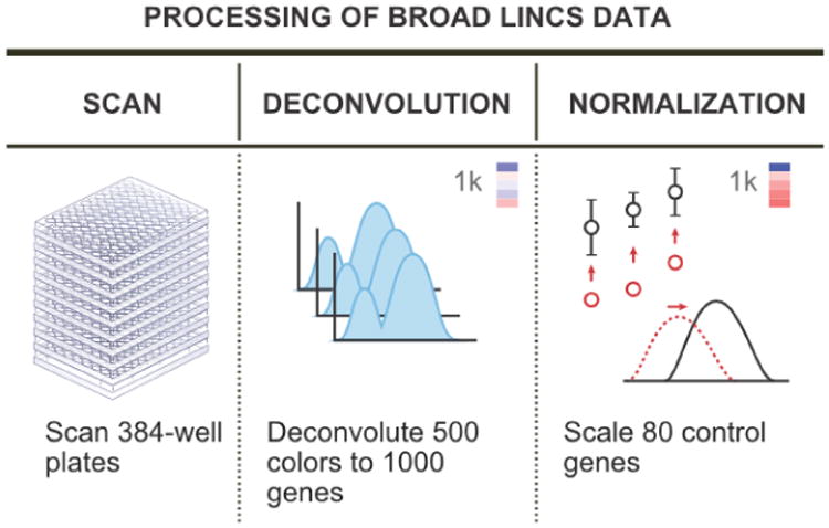
The L1000 data preprocessing pipeline. The raw data are first measured from the beads in the experiments. Next, the data from each color of bead are deconvolved to assign expression values to the two genes which share that bead color. Finally, the data are normalized to yield directly comparable data across experiments. Figure adapted from an image on the Broad Institute LINCS cloud website (http://lincscloud.org/l1000).

Although these data processing steps result in data that are more amenable to statistical analysis, we have found that the deconvolution step in particular introduces artifacts in the data. This can be seen when we look at multiple experiments on the same cell line with the same experimental conditions. If we look at a pair of genes that share a bead color and form a scatterplot of their values across many experiments, we see that these artifacts can take several forms.

First of all, two genes that are paired on the same bead color may not be expressed at levels such that they are easily distinguished. This can lead to both genes being assigned the same value, resulting in a clustering of data directly on the x = y diagonal. Secondly, the deconvolution step, which uses a simple k-means algorithm, can be misled if there are many beads sampled with very low fluorescence values. This, combined with the quantile normalization step, can lead to additional clusters that are not at the true expression value. Finally, the deconvolution step can result in assigning the expression levels of the genes incorrectly. That is, the expression level of gene A of the pair on the same bead color is sometimes assigned to gene B instead, and vice versa. Figure 2 shows examples of the raw bead data of two gene pairs and illustrates the difficulty of the deconvolution step.

Fig 2.

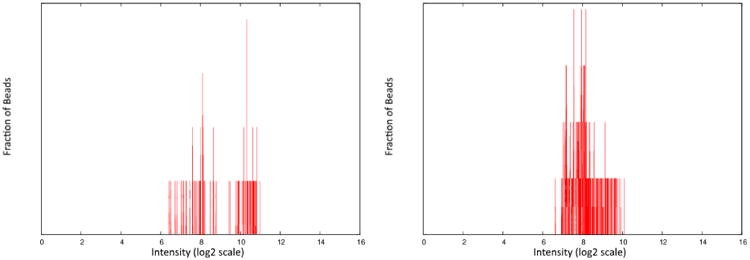
Histograms of raw bead fluorescence values for single bead colors. The left panel shows an example where the two peaks corresponding to the genes sharing the bead color are relatively easy to distinguish. The right panel shows an example where the deconvolution is more difficult. Dotted lines show possible inferred densities for two clusters.

Figure 3 shows examples of these three types of artifact in the L1000 data. The figure shows the expression values for two paired genes, CTLC and IKZF1. Each point shows the values measured in a single experiment. All 630 experiments in this dataset are on the same cell line, A375, and are untreated, used as controls. As such, we would expect a single cloud of observations centered around the point defined by the true expression values of the two genes. Instead, we see several clusters of observations, as well as points lying on or very near the diagonal. Note in particular the two circled sets of points. These appear to be a single cluster in which some of the points were flipped, with the expression values assigned to the wrong genes. If we flip one set of points across the diagonal, it falls directly on the other set.

Fig 3.

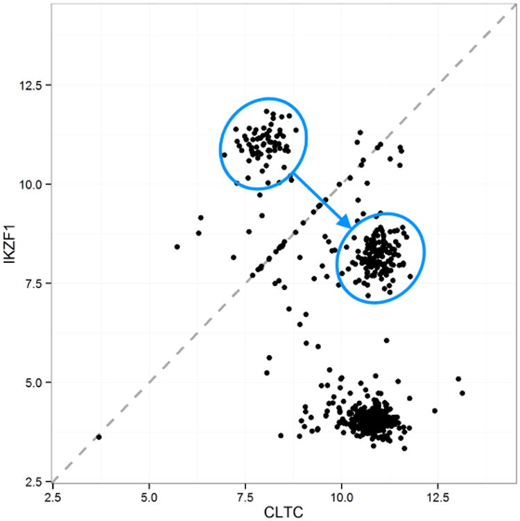
Expression levels on a log-base-2 scale for two paired genes, CLTC and IKZF1, measured on the same bead, in the L1000 data. Each point represents one experiment; there are 630 experiments in all. Data artifacts include points directly on or very near to the diagonal, multiple clusters rather than a single one as may be expected, and flipping between the two circled clusters of points, with the CLTC value incorrectly assigned to IKZF1, and vice versa. The blue arrow shows the effect of data correction using MCDC.

Looking more broadly at the untreated A375 experiments, we find that artifacts such as those in Figure 3 occur across gene pairs. Every pair of genes has at least a few points lying on or near the diagonal, with an average of about 30 per pair. If we compare the number of points on either side of the diagonal, excluding those close to it, we find that half of the gene pairs have at least 10% of the points on the wrong side of the diagonal (the side with fewer points), and a quarter of the pairs have at least 25% on the wrong side. This may be partially explained by gene pairs that have similar expression values, but the gene pairs were initially selected so as to avoid that problem.

3. Method

We propose a method to detect and correct all three kinds of artifact present in the LINCS L1000 data: the multiple clusters introduced by the preprocessing pipeline, the erroneous assignment of the same expression value to paired genes, and the flipping of the expression levels of paired genes. This improves the quality of the data and leads to better downstream analysis. We do this by addressing issues present in the preprocessed data rather than by reprocessing the raw data, as was done by Liu et al. (2015). We adopt this approach because some of the artifacts are likely to persist even if the deconvolution method is improved for individual gene pairs.

Our method is an extension of model-based clustering (Wolfe, 1970; Banfield and Raftery, 1993; McLachlan and Peel, 2000; Fraley and Raftery, 2002), which is a model-based method for finding clusters by fitting a multivariate Gaussian mixture model to the data. It has been found useful in many different contexts, including geochemical analysis (Templ et al., 2008), chemometrics (Fraley and Raftery, 2007), and health studies (Flynt and Daepp, 2015). It is well adapted to estimating the expression levels because sometimes there are small groups of points not in the main cloud around the true value, such as the points on the diagonal in Figure 3. Model-based clustering can identify these groups as clusters and remove or downweight them, thus preventing them from contaminating the estimation of the gene expression levels.

However, while model-based clustering is able to identify the clusters as well as identifying outliers, it does not have a mechanism for identifying particular points as flipped. Here we extend the model-based clustering method to detect and take into account the flipping in the data. More generally, it can be used for data with any invertible transformation applied to a subset of the data. This extension allows us to use an Expectation-Maximization (EM) algorithm commonly used to estimate finite mixture models (Dempster et al., 1977; McLachlan and Krishnan, 1997).

3.1. Model

Suppose we have multivariate data, {x_i : i = 1, …, N}, generated by a finite mixture of G distributions f_k, k = 1, …, G with probabilities τ₁, …, τ_G:

$$f(\mathbf{x})=\sum _{k=1}^G{\tau }_k{f}_k(\mathbf{x}|{\theta }_k).$$

Suppose further that we do not observe x_i, but rather y_i, a possibly transformed version of x_i, where the probability of a data point having been transformed can depend on the mixture component k that x_i is drawn from:

$${\mathbf{y}}_i=\{\begin{array}{cc}{\mathbf{x}}_i& \text{with probability}{\pi }_k,\\ {\mathbf{\text{Tx}}}_i& \text{with probability}(1-{\pi }_k).\end{array}$$

Here, T is any invertible transformation that preserves the domain of x. Often, this may be represented as a matrix, but it may also be a functional transformation (i.e. a component-wise monotonic transformation). In the case of the L1000 data, this is just the 2×2 matrix with zeros on the diagonals and ones on the off-diagonals, switching the two values. Given the transformation T, the distribution of y_i can be written as follows:

$$f({\mathbf{y}}_i|\mathit{\tau },\mathit{\pi },\mathit{\theta })=\sum _{k=1}^G{\tau }_k[{\pi }_k{f}_k({\mathbf{y}}_i|{\theta }_k)+(1-{\pi }_k)f_k({\mathbf{T}}^{-1}{\mathbf{y}}_i|{\theta }_k)].$$

To simplify the notation, define f_ik ≡ f_k(y_i|θ_k) and $f_{ik}^{-}\equiv f_k({\mathbf{T}}^{-1}{\mathbf{y}}_i|{\theta }_k)$. Then the distribution of y_i can be written

$$f(\mathbf{y}|\mathit{\tau },\mathit{\pi },\mathit{\theta })=\prod _{i=1}^n\sum _{k=1}^G{\tau }_k[{\pi }_k{f}_{ik}+(1-{\pi }_k)f_{ik}^{-}].$$

3.2. EM Algorithm

We estimate this model by maximum likelihood using the EM algorithm. We formulate this as a missing data problem where the complete data are {y_i, z_i, ξ_i}. Here, z_i = (z_i1, …, z_iG) and ξ_i are unobserved labels, with

$$z_{ik}=\{\begin{array}{cc}1& \text{if}{\mathbf{y}}_i\text{belongs to group}k,\\ 0& \text{otherwise},\end{array}$$

and

$${\xi }_i=\{\begin{array}{cc}0& \text{if}{\mathbf{y}}_i\text{has been transformed},\\ 1& \text{otherwise}.\end{array}$$

Then the complete-data log-likelihood is

$$l(\mathit{\theta },\mathit{\tau },\mathbf{z},\mathit{\pi },\mathit{\xi }|\mathbf{y})=\sum _{i=1}^n\sum _{k=1}^G{z}_{ik}[{\xi }_{i}log({\pi }_k{\tau }_k{f}_{ik})+(1-{\xi }_i)log((1-{\pi }_k){\tau }_k{f}_{ik}^{-})].$$

We can also write down the joint distribution of z_i and ξ_i given y_i and θ:

$$f({\mathbf{z}}_i,{\mathbf{\xi }}_i|{\mathbf{y}}_i,\mathit{\theta })=\frac{1}{f({\mathbf{y}}_i|\mathit{\tau }\mathit{,}\mathit{\pi },\mathit{\theta })}\prod _{k=1}^G{[{({\tau }_k{\pi }_k{f}_{ik})}^{{\xi }_i}\cdot {({\tau }_k(1-{\pi }_k)f_{ik}^{-})}^{(1-{\xi }_i)}]}^{z_{ik}}.$$ (1)

For the E-step of the algorithm, we need to calculate the expected complete-data log-likelihood, namely

$$\begin{array}{c}Q(\mathit{\theta }|{\mathit{\theta }}^{\ast })=E[l(\mathit{\theta },\mathit{\tau },\mathbf{z},\mathit{\pi },\mathit{\xi }|\mathbf{y})|\mathbf{y},{\mathit{\tau }}^{\ast },{\mathit{\pi }}^{\ast },{\mathit{\theta }}^{\ast }],\\ =\sum _{i=1}^n\sum _{k=1}^{G}E[z_{ik}{\xi }_i|\mathbf{y},{\mathit{\tau }}^{\ast },{\mathit{\pi }}^{\ast },{\mathit{\theta }}^{\ast }]log({\pi }_k{\tau }_k{f}_{ik})+E[z_{ik}(1-{\xi }_i)|\mathbf{y},{\mathit{\tau }}^{\ast },{\mathit{\pi }}^{\ast },{\mathit{\theta }}^{\ast }]log((1-{\pi }_k){\tau }_k{f}_{ik}^{-}).\end{array}$$

From Equation (1), we have

$$\begin{array}{c}E[z_{ik}{\xi }_i|\mathbf{y},{\mathit{\tau }}^{\ast },{\mathit{\pi }}^{\ast },{\mathit{\theta }}^{\ast }]=\frac{{\tau }_k^{\ast }{\pi }_k^{\ast }{f}_{ik}}{f({\mathbf{y}}_i|{\mathit{\tau }}^{\ast },{\mathit{\pi }}^{\ast },{\mathit{\theta }}^{\ast })},\\ E[z_{ik}(1-{\xi }_i)|\mathbf{y},{\mathit{\tau }}^{\ast },{\mathit{\pi }}^{\ast },{\mathit{\theta }}^{\ast }]=\frac{{\tau }_k^{\ast }(1-{\pi }_k^{\ast })f_{ik}^{-}}{f({\mathbf{y}}_i|{\mathit{\tau }}^{\ast },{\mathit{\pi }}^{\ast },{\mathit{\theta }}^{\ast })}.\end{array}$$

We have z_ikξ_i + z_ik(1 – ξ_i) = z_ik and ${\sum }_{k=1}^G{z}_{ik}=1$. This leads to the following updates of the estimates of z_ik and ξ_i, which make up the E-step:

$$\begin{array}{c}{\widehat{z}}_{ik}=\frac{{\tau }_k^{\ast }[{\pi }_k^{\ast }{f}_{ik}+(1-{\pi }_k^{\ast }{f}_{ik}^{-})]}{f(y_i|{\mathit{\tau }}^{\ast },{\mathit{\pi }}^{\ast },{\mathit{\theta }}^{\ast })},\\ {\widehat{\xi }}_i=\frac{{\sum }_{k=1}^G{\tau }_k^{\ast }{\pi }_k^{\ast }{f}_{ik}}{f(y_i|{\mathit{\tau }}^{\ast },{\mathit{\pi }}^{\ast },{\mathit{\theta }}^{\ast })}.\end{array}$$

The M-step is then as follows:

$$\begin{array}{c}{\widehat{\tau }}_k\leftarrow \frac{n_k}{n},\\ {\widehat{\pi }}_k\leftarrow \frac{{\sum }_{i=1}^n{\widehat{z}}_{ik}{\widehat{\xi }}_i}{n_k},\\ {\widehat{\mathit{\mu }}}_k\leftarrow \frac{{\sum }_{i=1}^n{\widehat{z}}_{ik}({\widehat{\xi }}_i{\mathbf{y}}_i+(1-{\widehat{\xi }}_i){\mathbf{T}}^{-1}{\mathbf{y}}_i)}{n_k},\\ n_k\equiv \sum _{i=1}^n{\widehat{z}}_{ik}.\end{array}$$

To get the variance of the clusters, we follow the steps from Celeux and Govaert (1995), modifying the scattering matrix W_k of cluster k as well as the within-cluster scattering matrix W to be

$$\begin{array}{c}{W}_k=\sum _{i=1}^n{\widehat{z}}_{ik}[{\widehat{\xi }}_i({\mathbf{y}}_i-{\widehat{\mathit{\mu }}}_k){({\mathbf{y}}_i-{\widehat{\mathit{\mu }}}_k)}^{\prime }+(1-{\widehat{\xi }}_i)({\mathbf{T}}^{-1}{\mathbf{y}}_i-{\widehat{\mathit{\mu }}}_k){({\mathbf{T}}^{-1}{\mathbf{y}}_i-{\widehat{\mathit{\mu }}}_k)}^{\prime }],\\ W=\sum _{k=1}^G{W}_k.\end{array}$$

These can then be used to calculate Σ_k under different variance models.

We iterate the EM steps until convergence, which leads to a local maximum of the log-likelihood (Wu, 1983). Although this is not guaranteed to be the global maximum, choosing starting values using hierarchical model-based clustering, or doing multiple restarts, have both been shown to lead to good solutions (Fraley and Raftery, 1998; Biernacki et al., 2003).

Our model allows the cluster-specific variance matrices to differ between clusters. We select the best number of clusters by running MCDC with the number of clusters ranging from 1 to some maximum number of clusters (9 in our case) and then comparing the BIC values for the resulting estimated models (Fraley and Raftery, 2002).

For our gene expression data, we estimate the expression levels of a pair of genes as the mean of the largest cluster (the cluster with the most points assigned to it) found using the chosen model. This gives a reasonable estimate - we expect the data points to be distributed about a single true value since the experiments were done under the same conditions and the observations come from a culture of a large number of cells.

4. Simulation Study

We now describe a simulation study in which data with some of the key characteristics of the LINCS L1000 data were simulated. We simulated datasets with no clustering (i.e. one cluster), but where some of the observations were flipped. We also simulated datasets with clustering (two clusters), where some of the observations were flipped.

Finally, we simulated a dataset where no observations were flipped, but instead some observations were rotated and scaled. This is to show that the method can be effective when some of the data are perturbed in ways other than flipping.

4.1. Simulation 1: One Cluster With Flipping

Figure 4 is an example dataset from our first simulation. This simulation represents what we see in the LINCS L1000 data in the best case, with no clustering or diagonal values (i.e. a single cluster), but with some flipping. For the simulation, we generated 100 datasets with 300 points each from the single cluster model with flipping probabilities (1 – π) of 0.05 to 0.45 in increments of 0.05, resulting in 900 simulated data sets in total. We applied MCDC to each simulated dataset and counted the number of times the correct number of clusters (one) was selected as well as the percentage of the points correctly identified as flipped or not. Finally, we looked at the inferred gene means compared to taking the mean of all the observations without applying MCDC. We refer to this as the unaltered mean.

Fig 4.

One Dataset from Simulation 1: One Cluster with Flipping. The fraction of data flipped, 1 – π, is chosen to be 0.05. Left panel: Original data with flipped data points. Right panel: Data after correction by MCDC. MCDC identified and corrected all the flipped points. The grey triangle is the mean of all the data, and the yellow triangle is the mean of the data after correction by MCDC.

The correct number of clusters (i.e. one) was selected for all but one of the 900 datasets, and in the one erroneous dataset out of 900 only a few points were in a second cluster. In 858 of the 900 datasets no errors were made — all the points were correctly identified as being flipped or not flipped. In three datasets, all with the highest probability of flipping, namely 0.45, all the points were misidentified by being flipped to the wrong side, while in one dataset (again with 1 – π = 0.45), a single large cluster with no flipping was identified. In the remaining 38 datasets, one to three points out of 300 were misidentified. All these misidentifications make sense, since we expect rare cases where a point crosses the x = y line as well as cases where more points are flipped when using a flipping probability near 0.5.

Figure 5 and Table 1 show the mean absolute error in inferred mean using MCDC versus the unaltered data. For each flipping probability, we calculated the mean absolute error of the inferred mean from the true mean. MCDC did much better than taking the unaltered mean in all cases, improving on the unaltered data by a factor of 5 to 36, depending on the probability of flipping.

Fig 5.

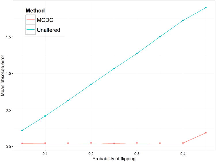
Simulation 1: Mean Absolute Error in Inferred Mean. The blue line is based on using unaltered data, while the red line is based on using the mean of the largest cluster found by MCDC.

Table 1.

Simulation 1: Mean Absolute Error (MAE) in Inferred Mean for Unaltered data and MCDC-corrected Data, as the probability of flipping increases. The MAE ratio is the ratio of mean absolute error using the unaltered data divided by the MAE using the MCDC-corrected data. Values greater than 1 indicate improvement by using MCDC.

Probability of Flipping	Unaltered MAE	MCDC MAE	MAE Ratio
0.05	0.22	0.04	5
0.10	0.42	0.05	9
0.15	0.63	0.05	13
0.20	0.85	0.05	17
0.25	1.07	0.05	24
0.30	1.27	0.05	25
0.35	1.50	0.05	32
0.40	1.73	0.05	36
0.45	1.90	0.19	10

4.2. Simulation 2: Two Clusters with Flipping

For the second simulation, we added a second cluster on the diagonal, as demonstrated in Figure 6. This reflects a common issue we see in the L1000 data. When the data processing pipeline has trouble differentiating between the two gene expression levels, it can end up assigning them both the same value. For these data, we wanted to see how well MCDC identified the “good” points (not the diagonal cluster). Again, we used the mean of the largest cluster as the inferred mean. For the simulation, we generated 100 datasets with 400 points each for the two-cluster model with flipping probabilities (1 – π) from 0.05 to 0.45, and probability τ of a point being in the true cluster from 0.55 to 0.95, in increments of 0.05.

Fig 6.

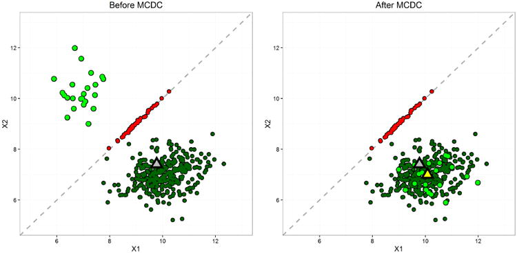
Simulated dataset 2: two clusters after flipping. For this example, 90% of the data fall in the main cluster, and the fraction of points in the main cluster that were flipped, 1 – π, is chosen to be 0.05. MCDC correctly identified the two clusters and the flipped points, as seen in the plot on the left. The grey triangle is the mean of all the data, which is moved from its true position due to the second cluster. The yellow triangle is the mean of the largest cluster found by MCDC and is much closer to the true value.

Figure 7 shows the comparison of mean absolute error in the inferred mean. The MCDC results are better across the board, although we see that as τ decreases, it is more likely to identify the diagonal cluster as the largest one. Figure 8 shows that MCDC does well in identifying which points are flipped. In Figure 9, we see that the correct number of clusters is not generally identified as well as we might like. This may be due to poor initialization of the algorithm and may be corrected with multiple random initializations.

Fig 7.

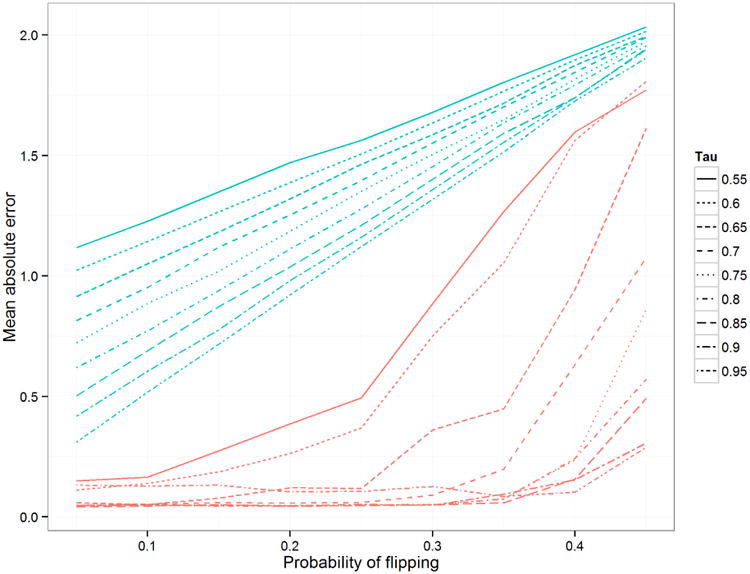
Mean absolute error in inferred mean comparison for simulation 2 when varying τ, the probability that a point comes from the primary cluster. The blue line is using unaltered data, while the red line is using the mean of the largest cluster found by MCDC.

Fig 8.

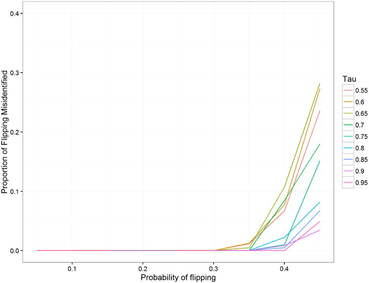
Proportion of points correctly identified as flipped or not flipped for simulation 2 when varying τ, the probability that a point comes from the primary cluster. When there is a high probability of flipping (near 0.5), there may be more points in the flipped cluster, leading to MCDC identifying it as the main cluster and thus misidentifying all points for a particular dataset.

Fig 9.

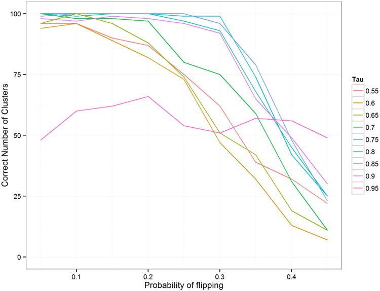
Number of datasets (out of 100) in which 2 clusters was identified as the best result for simulation 2 when varying τ, the probability that a point comes from the primary cluster. When τ was high, MCDC did not always correctly identify the cluster on the diagonal due to the low number of points in that cluster.

4.3. Simulation 3: Three Clusters With Rotation and Scaling

To show that MCDC can be applied to other kinds of data errors than flipping, we also generated a dataset with three clusters where the error process rotates and scales the data points affected. This transformation is not motivated by the L1000 data but rather serves to demonstrate the potential for MCDC to be used in other situations. In this more complex situation we used n = 1000 points split among the three clusters with varying probabilities of transformation. MCDC selected the correct number of clusters and correctly classified all the points. Figure 10 shows the original and MCDC-corrected data. One caveat is that here, as in the flipping situation, the data error process was known to the MCDC algorithm.

Fig 10.

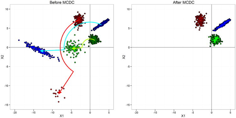
Simulation dataset 3: three clusters with rotation and scaling. A data point was transformed by rotating it 120° counter-clockwise around the origin and then scaling out from the origin by a factor of 2, as seen in the plot on the left. MCDC was able to identify the correct clusters and assign the transformed points back into the appropriate clusters, as on the right.

5. Application to LINCS L1000 Data

We applied MCDC to a portion of the LINCS L1000, namely the data from cell line A375, a human skin malignant melanoma cell line. We chose this cell line because it had good coverage in the L1000 data in terms of the number of different perturbations applied. We considered only the transformation T that switches the expression levels of the paired genes. We looked at improvement of the data in aggregate as well as improvement in a specific inferential setting. For each pair of genes, we ran MCDC with 1 to 9 clusters on 2,044 untreated experiments and chose the optimal number of clusters by BIC. Running this on a laptop with a 2.6GHz Intel i7-6700HQ processor took approximately 47 minutes on a single core for all gene pairs, or under 6 seconds for running MCDC with each of 1 to 9 clusters on a single gene pair. The running time could be improved by running MCDC on the gene pairs in parallel.

Three gene pairs were selected to illustrate the results of applying MCDC to the L1000 data. Figure 11 shows the results of applying MCDC to one gene pair in the untreated experiments in cell line A375. Each point corresponds to a single experiment, and most of the points fall in the same region. However, there is a single point in the top-left corner that appears to be mirrored across the x = y line, and we suspect that this point has had the expression levels of the two genes switched. MCDC corrects this point and we see that it does indeed fall within the main body of points.

Fig 11.

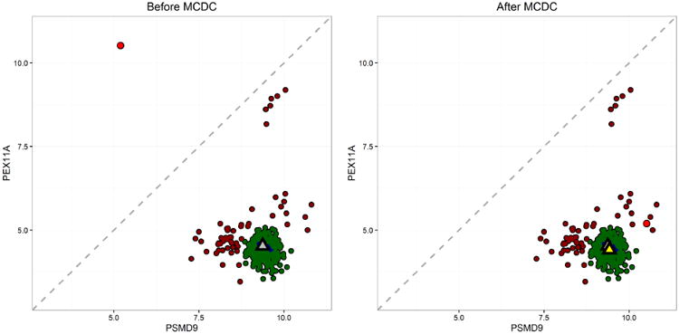
Example 1 showing the results of applying MCDC to L1000 control data. MCDC chooses 3 clusters by BIC. On the left are the data before correction, and on the right are the same data after correction. Triangles indicate inferred mean - gray is the mean of all the data while yellow is the mean of the largest cluster found by MCDC.

Note that here that the best solution by BIC involves three clusters. This means that the distribution of the points may not be strictly normal, but here the components overlap such that they form one contiguous cluster.

Figures 12 and 13 show MCDC applied to additional gene pairs in the same dataset. In each case MCDC succeeded in removing the artifacts in the data. MCDC selects 3 clusters in Figure 12 and 5 clusters in Figure 13. Note in Figure 13 that the inferred mean after MCDC is substantially different than the mean of the full dataset moving it from a location not near any data to one within the largest cluster. Figure 14 shows the distribution of the number of clusters chosen by BIC across all the gene pairs.

Fig 12.

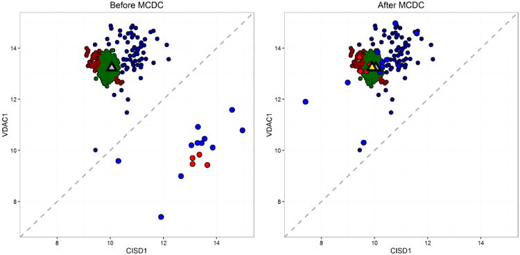
Example 2 showing the results of applying MCDC to L1000 control data. MCDC chooses 3 clusters by BIC. On the left is the data before correction, and on the right is the same data after correction. Triangles indicate inferred mean - gray is the mean of all the data while yellow is the mean of the largest cluster found by MCDC.

Fig 13.

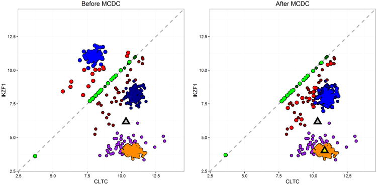
Example 3 showing the results of applying MCDC to L1000 control data. MCDC chooses 5 clusters by BIC. On the left is the data before correction, and on the right is the same data after correction. Triangles indicate inferred mean - gray is the mean of all the data while yellow is the mean of the largest cluster found by MCDC.

Fig 14.

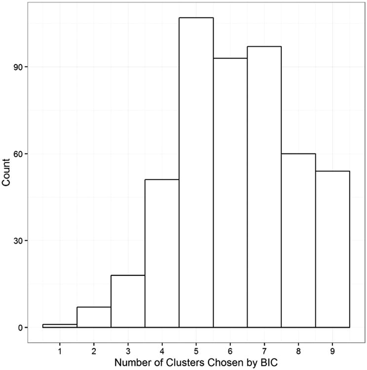
Histogram of the numbers of clusters chosen by BIC for the gene pairs.

5.1. Agreement with External Baseline Data

We wanted to see if MCDC improves the data relative to an external baseline. There are 2,044 untreated experiments in the A375 cell line. These experiments should all yield similar expression levels since they are all done under the same experimental conditions. We can get an estimate of the gene expression level of a particular gene by taking the mean across all the experiments. We refer to this as the unaltered data.

There are two expression level baseline datasets included in the LINCS L1000 metadata for cell line A375, one using RNAseq technology and the other using Affymetrix microarray technology. Each of these datasets was generated using an independent technology and can be compared to the values in the L1000 data. Since the baseline datasets were produced using different technologies, the scales of the expression levels are different from that from the L1000 data. In order to take this difference into account, we looked at the mean squared error (MSE) from a simple linear regression of the baseline data on the inferred gene expression levels from the L1000 data.

We then applied MCDC to see if this improved the estimates of gene expression. To do this, we applied MCDC separately to each pair of genes that were measured using the same bead color. For a gene pair, we ran MCDC on the data from the 2,044 experiments. Doing this for all 500 gene pairs, we ended up with an estimated gene expression level for all of the 1,000 landmark genes. These estimates were also compared to the baseline estimates and we were able to compare the MSEs of the unaltered data with those from the corrected data.

Liu et al. (2015) introduced a new processing pipeline for the LINCS L1000 data in order to address some of the issues they found with the data. They started with the raw data and performed the deconvolution step with a Gaussian mixture model approach rather than the k-means approach used in the original pipeline. This yielded what they refer to as Level 2 data, which they then further normalized and performed quality control on to produce Level 3 data. The Liu Level 2 data can be compared with the Level 3 data from the L1000 pipeline, while the Liu Level 3 data is similar to the Level 4 L1000 data.

As a comparison with MCDC, we looked at the same regression against the Affymetrix and RNAseq baselines using the mean values from the Liu Level 2 data for each gene, again for the A375 untreated experiments. We used the Liu Level 2 data because part of the process of creating the Level 3 data removes the means from the gene data, which is not useful for our purpose. The Liu data included observations from 532 experiments.

Table 2 shows the results of this analysis. Using the corrected data improved the MSE by 8% when using the Affymetrix data and by 7% when using the RNAseq data. The Liu data also improved the MSEs, though not as much as MCDC in the case of the Affymetrix baseline.

Table 2.

MSE of regressing external baseline data on imputed gene means. Comparison of unaltered means, means from the Liu data, and MCDC data. Affymetrix and RNAseq baselines are both from external sources independent of the LINCS L1000 data.

Method	Affymetrix Baseline	RNAseq Baseline
Unaltered	1.91	1.66
Liu	1.87	1.58
MCDC	1.76	1.55

It is also of interest to note that the performance of MCDC in improving gene expression estimates does not depend on the number of clusters inferred. This is shown in Figure 15, where we look at the improvement in the residual for each gene from the regression using the unaltered means versus the regression using the MCDC-corrected estimates. Figure 15 shows the results when using the Affymetrix baseline; the results were similar with the RNAseq baseline. There is not a substantial change in the improvement based on whether a small or large number of clusters is chosen.

Fig 15.

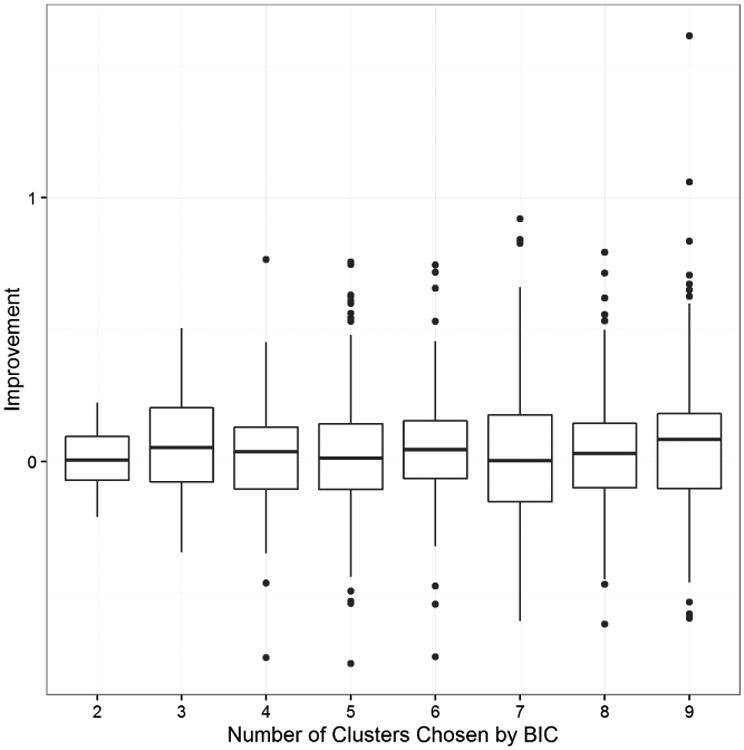
Boxplots showing the improvement in gene expression estimation for each gene versus the Affymetrix baseline, by the number of clusters chosen. Improvement is calculated as the absolute residual from regression using the original data minus the absolute residual from regression using the MCDC estimates. Positive values indicate improvement from using MCDC.

5.2. Gene Regulatory Network Inference

As well as improving the overall estimates of gene expression levels, MCDC identifies particular experiments where the gene pairs are flipped. This improvement in the data leads to improvements in methods that use the data in a more granular way. One common use for gene expression datasets is to infer gene regulatory networks.

Gene regulatory networks describe the connectedness of genes within the cell. Understanding these genetic interactions leads to understanding of how organisms function and develop at a cellular level. Many methods have been developed for inferring these relationships. These include stochastic methods such as mutual information (Basso et al., 2005; Faith et al., 2007; Margolin et al., 2006; Meyer et al., 2007), linear models (Gustafsson et al., 2009; Lo et al., 2012; Menéndez et al., 2010; Young et al., 2014), and Bayesian networks (Kim et al., 2003; Murphy and Mian, 1999; Zou and Conzen, 2005), as well as deterministic methods involving systems of differential equations (Bansal et al., 2006; D'haeseleer et al., 1999).

To assess the improvement from MCDC, we looked at inferring gene regulatory networks from the LINCS L1000 data knockdown experiments, which target a specific gene to suppress its expression level. This target gene is the regulator in these experiments, and the remaining genes are potential targets, giving us a causal pathway by which to infer networks.

We previously developed a simple posterior probability approach using knockdown data to infer edges (Young et al., 2016). To do this, we first standardized the knockdown data using the untreated experiments on the same plate to obtain z-values. We then used a simple linear regression model, regressing each potential target on the knocked down gene. Using Zellner's g-prior (Zellner, 1986), the posterior probability p_ht of there being an edge from the knocked-down gene h to the target gene t is

$$\begin{array}{c}{p}_{ht}=\frac{T_{ht}}{1+T_{ht}},\text{where}\\ T_{ht}=\frac{{\pi }_{ht}}{1-{\pi }_{ht}}exp[(n_h-2)log(1+g)/2-(n_h-1)log(1+g(1-R^2))/2].\end{array}$$ (2)

In (2), R² is the coefficient of determination for the simple linear regression model, g is from Zellner's g-prior, π_ht is the prior probability of an edge between h and t, and n_h is the number of knockdown experiments. For our data, we used π_ht = 0.0005, reflecting the average expected number of regulators, and chose g = √n, a value we have previously found to be reasonable (Young et al., 2014). This approach is fast and allows us to incorporate prior probabilities as well. The final result is a ranked edgelist.

The LINCS L1000 data include multiple knockdown experiments for most of the landmark genes. Most genes have between 9 and 15 replicates with some having as few as 4 or as many as 100. This limits the effectiveness of MCDC for this data, but we were still able to apply it to many of the knockdown datasets.

We used the posterior probability method on the knockdown experiments for cell line A375 to generate a ranked list of potential edges. In order to assess the results, we used a gene-set library compiled from TRANSFAC and JASPAR (Wingender et al., 2000; Sandelin et al., 2004) and accessed from Enrichr at http://amp.pharm.mssm.edu/Enrichr/ (Chen et al., 2013a). This is a list of transcription factors, namely genes that are known to control the expression levels of other genes. Each transcription factor has a list of target genes, yielding an assessment edgelist.

The TRANSFAC and JASPAR (T&J) edgelist is not a complete list since not all gene relationships are captured in the T&J library. This is in part because the T&J data focus on transcription factors, but also because the true regulatory networks are not fully known. The T&J edgelist includes edges for 37 transcription factors also found among the LINCS landmark genes. This includes 4,193 regulator-target pairs out of 43,290 potential edges for which we computed posterior probabilities.

To see the benefit from using MCDC, we applied the posterior probability method using the unaltered data and compared the results with using the same posterior probability method on the data after it had been corrected using MCDC. This results in two ranked lists of gene pairs with associated posterior probabilities. We compare these with the T&J assessment dataset by taking all edges with a posterior probability over a specified cutoff and creating two-by-two tables showing how well the truncated edgelists overlap with the T&J edgelist.

Table 3 shows the two-by-two tables generated at posterior probability cutoffs of 0.5 and 0.95. We also report approximate p-values by using the probability of getting at least the number of true positives found using a binomial(n, p) distribution, where n is the number of pairs in the inferred list and p is the probability of selecting a true edge from the total number of possible edges. From the table, we can see that the p-value is better for the corrected data at both probability cutoffs. The corrected data include more edges at both cutoffs but maintain a similar precision, defined as the proportion of edges which are true edges.

Table 3.

Two by two tables for cell line A375 using knockdown experiments for finding edges, compared to TRANSFAC and JASPAR from Enrichr. When using the unaltered data and looking at edges with posterior probability of 0.5 or greater, 41 of the 302 candidate edges are found in TRANSFAC and JASPAR, and 14 of the 81 candidate edges at a cutoff of 0.95 are true edges. Similarly, when using the MCDC-corrected data, 63 of the 463 candidate edges at a cutoff of 0.5 are true edges and 20 of the 119 at a cutoff of 0.95 are true edges. Approximate binomial p-values are included.

		T&J
		cutoff: 0.5		cutoff: 0.95
		Yes	No	Yes	No
Unaltered	Yes	41	261	14	67
	No	4152	38836	4179	39030
		p-value: 0.02		p-value: 0.02
MCDC	Yes	63	400	20	99
	No	4130	38697	4173	38998
		p-value: 0.004		p-value: 0.01

Another way of looking at the results is via the precision-recall curve (Raghavan et al., 1989). Precision and recall are both calculated by truncating our ranked list of edges and looking only at the edges in the truncated list. The precision is the proportion of the edges in the truncated list which are true edges. Recall is defined as the proportion of all true edges which are in the truncated list. The precision-recall curve takes a ranked list of edges from a procedure and shows how the precision varies as more edges are included from the list. High precision at low recall indicates that the procedure is good at identifying true edges at the highest probability. This is important in many cases, particularly genetic studies, because it gives researchers good information on where to focus their efforts in subsequent studies.

Figure 16 compares the precision-recall curves for the unaltered and corrected data at the very top of the edgelist. The dashed line shows what would be expected by randomly ordering the edges; anything above that line is an improvement. Both methods give improved results, but the corrected data yield much better results for the very top edges returned. This is of particular importance for further research because having high confidence in the top edges allows the biologist to develop further experiments to focus on these edges in additional, more targeted experiments. In this respect, data correction with MCDC provides substantial improvement.

Fig 16.

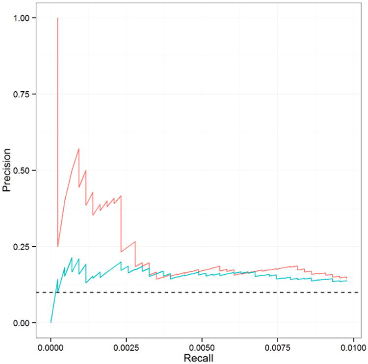
Precision-recall curve comparing edgelists from unaltered (blue line) and MCDC-corrected (red line) data on knock down data.

We can see this by looking at the inferred edges, ranked so that the first edge has the highest posterior probability, the second has the second highest, and so one. Table 4 is constructed by ranking the edgelist from the posterior probability method on a particular dataset. Thus the first edge in the list is the one with the highest posterior probability, the second edge has the next highest posterior probability, and so on. We then look at each edge and see if it is also found in the T&J assessment edgelist. The rank in the table indicates the position at with the n-th edge in T&J was found in the ranked edgelist. It can be seen that the edge with the highest posterior probability using the MCDC-corrected data is in T&J, as are the edges with the 5th, 6th, 7th and 10th highest posterior probabilities. Only one of the top 10 edges from the unaltered data is a true edge, namely the one with the 7th highest posterior probability, while, in contrast, five of the top ten edges from the MCDC-corrected data are true edges.

Table 4.

Comparison of the rank of the first 5 edges found that match the TRANSFAC and JASPAR edgelist. Edges ranked by posterior probability. MCDC-corrected data produces found edges at higher ranks than the uncorrected data. See text for explanation of how the table was constructed.

Found Edge	Unaltered Rank	MCDC Rank
1	7	1
2	11	5
3	14	6
4	19	7
5	26	10

We also applied the posterior probability method to the Liu Level 3 data. In this case, the Level 3 data is appropriate since it is more comparable to our z-value transformation, and quality control has been performed to improve the data. We used the same prior and choice of g as for the other datasets. Due to the quality control step employed by Liu, there were fewer experiments available and only 24,377 testable edges had posterior probabilities. Of these, 2,746 were in the T&J assessment dataset. None of the edges had a posterior probability over 0.95, and only two had a posterior probability of at least 0.5. Neither of these edges was in the T&J dataset. When we looked at the edges as ranked by posterior probability, we found that the edge with the 12th-highest posterior probability, at 0.04, was the first which was also found in T&J. The lack of high posterior probability edges and positive results using the Liu Leve 3 data is due in part to the quality control step used, which resulted in fewer observations for each knockdown data set.

6. Discussion

When working with any data, understanding the unique aspects of how it was generated and processed can be helpful in developing models and methods, leading to improved inference. This is particularly true with genomic data. There are often many steps of data transformation and normalization between the raw measured data and what is used by the researcher in drawing conclusions (Binder and Preibisch, 2008). When these steps are not known or understood, assumptions about sources of error can be misinformed and lead to degraded performance in inference. Price et al. (2006) identified population stratification of allele frequency in disease studies, while Gomez-Alvarez et al. (2009) found that a particular sequencing technique resulted in many artificial replicates. Lehmann et al. (2013) showed that quantile normalization of microarray data introduced a phase shift into time-series in strains of cyanobacteria, changing night-expressed genes into day-expressed genes and vice versa. Stokes et al. (2007) developed a tool to identify and remove artifacts in genomic data. Batch effects have been identified as a significant source of systematic error that can be corrected (Leek et al., 2010; Chen et al., 2011; Sun et al., 2011). Identifying these sources of error is crucial, and in some cases can lead to much improved results.

We have shown how understanding the data-processing pipeline of the LINCS L1000 data allowed us to identify the introduction of a particular error, namely the flipping of expression values for gene pairs. This led to the development of MCDC, which is able to identify and correct these flipping errors. We were able to apply MCDC to improve the L1000 data in aggregate, as measured against external standards. This improvement of the data also led to improved inference of regulatory relationships between the genes, in particular for the edges ranked highest. Moreover, the use of the EM algorithm for optimization makes MCDC fast and useful for large datasets.

We showed that MCDC compared favorably to the data from Liu et al. (2015) in our assessments, but it is important to note that our approach is orthogonal to theirs. As an example of this, Figure 17 shows the Liu Level 2 data for a gene pair in the untreated A375 data. We see that there is evidence that this data could benefit from MCDC as well, prior to the processing that creates the Level 3 data.

Fig 17.

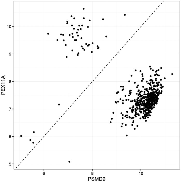
Expression levels for two paired genes in the untreated experiments for cell line A375 from the Liu Level 2 data (532 experiments), demonstrating that MCDC could potentially be useful in this processing pipeline as well as the original L1000 pipeline.

MCDC is an extension of model-based clustering, which has been used extensively in other analyses of genetic data, including image analysis of microarrays (Li et al., 2005) and sequence analysis (Verbist et al., 2015). One of the most common uses of model-based clustering in genetics is in finding meaningful groups among gene expression profiles across multiple experiments under different experimental conditions (cell sources, phases, applied drugs, etc.) (Siegmund et al., 2004; Jiang et al., 2004). This includes methods using Gaussian mixture models (Yeung et al., 2001), infinite mixture models (Medvedovic and Sivaganesan, 2002) and Bayesian hierarchical clustering (Cooke et al., 2011). Our use of MCDC as a step in improving data quality is complementary to these analysis methods. An implementation of our method will be made available as an R package, mcdc, on CRAN.

We showed in our simulation experiments that MCDC is able to accurately identify the data points which have been altered and thus improve the quality of the data. It is not limited to flipping, as seen in the LINCS data, but is able to handle any dataset where a subset of the data points have been altered in a known way. For the L1000 data, the transformation is informed by understanding the way the data is generated and pre-processed. In cases where there are multiple possibilities for T, it may be possible to run MCDC with each candidate transformation and compare the results to identify the one most compatible with the data.

References

- Ball CA, Sherlock G, Parkinson H, Rocca-Sera P, Brooksbank C, Causton HC, Cavalieri D, Gaasterland T, Hingamp P, Holstege F, Ringwald M, Spellman P, Stoeckert CJ, Stewart JE, Taylor R, Brazma A, Quackenbush J. Standards for microarray data. Science. 2002;298:539–539. doi: 10.1126/science.298.5593.539b. [DOI] [PubMed] [Google Scholar]
- Banfield JD, Raftery AE. Model-based Gaussian and non-Gaussian clustering. Biometrics. 1993;49:803–821. [Google Scholar]
- Bansal M, Della Gatta G, Di Bernardo D. Inference of gene regulatory networks and compound mode of action from time course gene expression profiles. Bioinformatics. 2006;22:815–822. doi: 10.1093/bioinformatics/btl003. [DOI] [PubMed] [Google Scholar]
- Basso K, Margolin AA, Stolovitzky G, Klein U, Dalla-Favera R, Califano A. Reverse engineering of regulatory networks in human B cells. Nature Genetics. 2005;37:382–390. doi: 10.1038/ng1532. [DOI] [PubMed] [Google Scholar]
- Biernacki C, Celeux G, Govaert G. Assessing a mixture model for clustering with the integrated completed likelihood. IEEE Transactions on Pattern Analysis and Machine Intelligence. 2000;22:719–725. [Google Scholar]
- Biernacki C, Celeux G, Govaert G. Choosing starting values for the EM algorithm for getting the highest likelihood in multivariate Gaussian mixture models. Computational Statistics and Data Analysis. 2003;41:561–575. [Google Scholar]
- Binder H, Preibisch S. “Hook”-calibration of Genechip-microarrays: Theory and algorithm. Algorithms for Molecular Biology. 2008;3:1–25. doi: 10.1186/1748-7188-3-12. [DOI] [PMC free article] [PubMed] [Google Scholar]
- Blocker AW, Meng XL. The potential and perils of preprocessing: Building new foundations. Bernoulli. 2013;19:1176–1211. [Google Scholar]
- Bolstad BM, Irizarry RA, Åstrand M, Speed TP. A comparison of normalization methods for high density oligonucleotide array data based on variance and bias. Bioinformatics. 2003;19:185–193. doi: 10.1093/bioinformatics/19.2.185. [DOI] [PubMed] [Google Scholar]
- Campbell JG, Fraley C, Stanford D, Murtagh F, Raftery AE. Model-based methods for textile fault detection. International Journal of Imaging Systems and Technology. 1999;10:339–346. [Google Scholar]
- Celeux G, Govaert G. Gaussian parsimonious clustering models. Pattern Recognition. 1995;28:781–793. [Google Scholar]
- Chen B, Greenside P, Paik H, Sirota M, Hadley D, Butte A. Relating chemical structure to cellular response: An integrative analysis of gene expression, bioactivity, and structural data across 11,000 compounds. CPT: Pharmacometrics & Systems Pharmacology. 2015;4:576–584. doi: 10.1002/psp4.12009. [DOI] [PMC free article] [PubMed] [Google Scholar]
- Chen C, Grennan K, Badner J, Zhang D, Gershon E, Jin L, Liu C. Removing batch effects in analysis of expression microarray data: an evaluation of six batch adjustment methods. PloS one. 2011;6:e17238. doi: 10.1371/journal.pone.0017238. [DOI] [PMC free article] [PubMed] [Google Scholar]
- Chen EY, Tan CM, Kou Y, Duan Q, Wang Z, Meirelles GV, Clark NR, Ma'ayan A. Enrichr: interactive and collaborative HTML5 gene list enrichment analysis tool. BMC Bioinformatics. 2013a;14 doi: 10.1186/1471-2105-14-128. article 128. [DOI] [PMC free article] [PubMed] [Google Scholar]
- Chen J, Hu Z, Phatak M, Reichard J, Freudenberg JM, Sivaganesan S, Medvedovic M. Genome-wide signatures of transcription factor activity: connecting transcription factors, disease, and small molecules. PLoS Comput Biol. 2013b;9 doi: 10.1371/journal.pcbi.1003198. article e1003198. [DOI] [PMC free article] [PubMed] [Google Scholar]
- Cooke EJ, Savage RS, Kirk PD, Darkins R, Wild DL. Bayesian hierarchical clustering for microarray time series data with replicates and outlier measurements. BMC Bioinformatics. 2011;12 doi: 10.1186/1471-2105-12-399. article 399. [DOI] [PMC free article] [PubMed] [Google Scholar]
- Crick F. Central dogma of molecular biology. Nature. 1970;227:561–563. doi: 10.1038/227561a0. [DOI] [PubMed] [Google Scholar]
- Dempster AP, Laird NM, Rubin DB. Maximum likelihood for incomplete data via the EM algorithm (with discussion) Journal of the Royal Statistical Society, Series B. 1977;39:1–38. [Google Scholar]
- D'haeseleer P, Wen X, Fuhrman S, Somogyi R. Pacific Symposium on Biocomputing. Vol. 4. World Scientific; 1999. Linear modeling of mRNA expression levels during CNS development and injury; pp. 41–52. [DOI] [PubMed] [Google Scholar]
- Duan Q, Flynn C, Niepel M, Hafner M, Muhlich JL, Fernandez NF, Rouillard AD, Tan CM, Chen EY, Golub TR, Sorger PK, Subramanian A, Ma'ayan A. LINCS Canvas Browser: interactive web app to query, browse and interrogate LINCS L1000 gene expression signatures. Nucleic Acids Research. 2014 doi: 10.1093/nar/gku476. page article gku476. [DOI] [PMC free article] [PubMed] [Google Scholar]
- Dunbar SA. Applications of Luminex® xMAP™technology for rapid, high-throughput multiplexed nucleic acid detection. Clinica Chimica Acta. 2006;363:71–82. doi: 10.1016/j.cccn.2005.06.023. [DOI] [PMC free article] [PubMed] [Google Scholar]
- Ellefsen KJ, Smith DB, Horton JD. A modified procedure for mixture-model clustering of regional geochemical data. Applied Geochemistry. 2014;51:315–326. [Google Scholar]
- Faith JJ, Hayete B, Thaden JT, Mogno I, Wierzbowski J, Cottarel G, Kasif S, Collins JJ, Gardner TS. Large-scale mapping and validation of Escherichia coli transcriptional regulation from a compendium of expression profiles. PLoS Biology. 2007;5 doi: 10.1371/journal.pbio.0050008. article e8. [DOI] [PMC free article] [PubMed] [Google Scholar]
- Flynt A, Daepp MI. Diet-related chronic disease in the northeastern United States: a model-based clustering approach. International Journal of Health Geographics. 2015;14:1–14. doi: 10.1186/s12942-015-0017-5. [DOI] [PMC free article] [PubMed] [Google Scholar]
- Fraley C, Raftery AE. How many clusters? Which clustering method? Answers via model-based cluster analysis. Computer Journal. 1998;41:578–588. [Google Scholar]
- Fraley C, Raftery AE. Model-based clustering, discriminant analysis, and density estimation. Journal of the American Statistical Association. 2002;97:611–631. [Google Scholar]
- Fraley C, Raftery AE. Model-based methods of classification: Using the mclust software in chemometrics. Journal of Statistical Software. 2007;18:1–13. [Google Scholar]
- Gomez-Alvarez V, Teal TK, Schmidt TM. Systematic artifacts in metagenomes from complex microbial communities. The ISME Journal. 2009;3:1314–1317. doi: 10.1038/ismej.2009.72. [DOI] [PubMed] [Google Scholar]
- Gustafsson M, Hörnquist M, Lundström J, Björkegren J, Tegnér J. Reverse engineering of gene networks with LASSO and nonlinear basis functions. Annals of the New York Academy of Sciences. 2009;1158:265–275. doi: 10.1111/j.1749-6632.2008.03764.x. [DOI] [PubMed] [Google Scholar]
- Ioannidis JP, Khoury MJ. Improving validation practices in ”omics” research. Science. 2011;334:1230–1232. doi: 10.1126/science.1211811. [DOI] [PMC free article] [PubMed] [Google Scholar]
- Jiang D, Tang C, Zhang A. Cluster analysis for gene expression data: A survey. IEE Transactions on Knowledge and Data Engineering. 2004;16:1370–1386. [Google Scholar]
- Kazor K, Hering AS. Assessing the performance of model-based clustering methods in multivariate time series with application to identifying regional wind regimes. Journal of Agricultural, Biological, and Environmental Statistics. 2015;20:192–217. [Google Scholar]
- Kim KH, Yun ST, Park SS, Joo Y, Kim TS. Model-based clustering of hydrochemical data to demarcate natural versus human impacts on bedrock groundwater quality in rural areas, South Korea. Journal of Hydrology. 2014;519:626–636. [Google Scholar]
- Kim SY, Imoto S, Miyano S. Inferring gene networks from time series microarray data using dynamic Bayesian networks. Briefings in Bioinformatics. 2003;4:228–235. doi: 10.1093/bib/4.3.228. [DOI] [PubMed] [Google Scholar]
- Leek JT, Johnson WE, Parker HS, Jaffe AE, Storey JD. The sva package for removing batch effects and other unwanted variation in high-throughput experiments. Bioinformatics. 2012;28:882–883. doi: 10.1093/bioinformatics/bts034. [DOI] [PMC free article] [PubMed] [Google Scholar]
- Leek JT, Scharpf RB, Bravo HC, Simcha D, Langmead B, Johnson WE, Geman D, Baggerly K, Irizarry RA. Tackling the widespread and critical impact of batch effects in high-throughput data. Nature Reviews Genetics. 2010;11:733–739. doi: 10.1038/nrg2825. [DOI] [PMC free article] [PubMed] [Google Scholar]
- Lehmann R, Machné R, Georg J, Benary M, Axmann IM, Steuer R. How cyanobacteria pose new problems to old methods: challenges in microarray time series analysis. BMC Bioinformatics. 2013;14 doi: 10.1186/1471-2105-14-133. article 133. [DOI] [PMC free article] [PubMed] [Google Scholar]
- Li Q, Fraley C, Bumgarner RE, Yeung KY, Raftery AE. Donuts, scratches and blanks: robust model-based segmentation of microarray images. Bioinformatics. 2005;21:2875–2882. doi: 10.1093/bioinformatics/bti447. [DOI] [PubMed] [Google Scholar]
- Liu C, Su J, Yang F, Wei K, Ma J, Zhou X. Compound signature detection on LINCS L1000 big data. Molecular BioSystems. 2015;11:714–722. doi: 10.1039/c4mb00677a. [DOI] [PMC free article] [PubMed] [Google Scholar]
- Liu X, Rattray M. Including probe-level measurement error in robust mixture clustering of replicated microarray gene expression. Statistical Applications in Genetics and Molecular Biology. 2010;9 doi: 10.2202/1544-6115.1600. article 42. [DOI] [PubMed] [Google Scholar]
- Lo K, Raftery AE, Dombek KM, Zhu J, Schadt EE, Bumgarner RE, Yeung KY. Integrating external biological knowledge in the construction of regulatory networks from time-series expression data. BMC Systems Biology. 2012;6 doi: 10.1186/1752-0509-6-101. article 101. [DOI] [PMC free article] [PubMed] [Google Scholar]
- Lockhart DJ, Dong H, Byrne MC, Follettie MT, Gallo MV, Chee MS, Mittmann M, Wang C, Kobayashi M, Horton H, Brown EL. Expression monitoring by hybridization to high-density oligonucleotide arrays. Nature biotechnology. 1996;14:1675–1680. doi: 10.1038/nbt1296-1675. [DOI] [PubMed] [Google Scholar]
- Margolin AA, Nemenman I, Basso K, Wiggins C, Stolovitzky G, Favera RD, Califano A. ARACNE: an algorithm for the reconstruction of gene regulatory networks in a mammalian cellular context. BMC Bioinformatics. 2006;7 doi: 10.1186/1471-2105-7-S1-S7. article S7. [DOI] [PMC free article] [PubMed] [Google Scholar]
- McLachlan GJ, Krishnan T. The EM Algorithm and Extensions. Wiley; 1997. [Google Scholar]
- McLachlan GJ, Peel D. Finite Mixture Models. Wiley; 2000. [Google Scholar]
- Medvedovic M, Sivaganesan S. Bayesian infinite mixture model based clustering of gene expression profiles. Bioinformatics. 2002;18:1194–1206. doi: 10.1093/bioinformatics/18.9.1194. [DOI] [PubMed] [Google Scholar]
- Menéndez P, Kourmpetis YA, ter Braak CJ, van Eeuwijk FA. Gene regulatory networks from multifactorial perturbations using Graphical Lasso: application to the DREAM4 challenge. PLoS One. 2010;5 doi: 10.1371/journal.pone.0014147. article e14147. [DOI] [PMC free article] [PubMed] [Google Scholar]
- Meyer PE, Kontos K, Lafitte F, Bontempi G. Information-theoretic inference of large transcriptional regulatory networks. EURASIP Journal on Bioinformatics and Systems Biology. 2007;2007:8–8. doi: 10.1155/2007/79879. [DOI] [PMC free article] [PubMed] [Google Scholar]
- Murphy K, Mian S. Technical report, Technical report, Computer Science Division. University of California; Berkeley, CA: 1999. Modelling gene expression data using dynamic Bayesian networks. [Google Scholar]
- Peck D, Crawford ED, Ross KN, Stegmaier K, Golub TR, Lamb J. A method for high-throughput gene expression signature analysis. Genome Biology. 2006;7 doi: 10.1186/gb-2006-7-7-r61. article R61. [DOI] [PMC free article] [PubMed] [Google Scholar]
- Price AL, Patterson NJ, Plenge RM, Weinblatt ME, Shadick NA, Reich D. Principal components analysis corrects for stratification in genome-wide association studies. Nature Genetics. 2006;38:904–909. doi: 10.1038/ng1847. [DOI] [PubMed] [Google Scholar]
- Raghavan V, Bollman P, Jung GS. A critical investigation of recall and precision as measures of retrieval system performance. ACM Transactions on Information Systems. 1989;7:205–220. [Google Scholar]
- Sandelin A, Alkema W, Engström P, Wasserman WW, Lenhard B. JASPAR: an open-access database for eukaryotic transcription factor binding profiles. Nucleic Acids Research. 2004;32:D91–D94. doi: 10.1093/nar/gkh012. [DOI] [PMC free article] [PubMed] [Google Scholar]
- Schena M, Shalon D, Davis RW, Brown PO. Quantitative monitoring of gene expression patterns with a complementary DNA microarray. Science. 1995;270:467. doi: 10.1126/science.270.5235.467. [DOI] [PubMed] [Google Scholar]
- Sebastiani P, Gussoni E, Kohane IS, Ramoni MF. Statistical challenges in functional genomics. Statistical Science. 2003;18:33–60. [Google Scholar]
- Shao H, Peng T, Ji Z, Su J, Zhou X. Systematically studying kinase inhibitor induced signaling network signatures by integrating both therapeutic and side effects. PLoS One. 2013;8 doi: 10.1371/journal.pone.0080832. article e80832. [DOI] [PMC free article] [PubMed] [Google Scholar]
- Siegmund KD, Laird PW, Laird-Offringa IA. A comparison of cluster analysis methods using DNA methylation data. Bioinformatics. 2004;20:1896–1904. doi: 10.1093/bioinformatics/bth176. [DOI] [PubMed] [Google Scholar]
- Stokes TH, Moffitt RA, Phan JH, Wang MD. Chip artifact CORRECTion (caCOR-RECT): a bioinformatics system for quality assurance of genomics and proteomics array data. Annals of Biomedical Engineering. 2007;35:1068–1080. doi: 10.1007/s10439-007-9313-y. [DOI] [PubMed] [Google Scholar]
- Sun Z, Wu Y, White WM, Donkena KV, Klein CJ, Garovic VD, Therneau TM, Kocher JPA. Batch effect correction for genome-wide methylation data with Illumina Infinium platform. BMC Medical Genomics. 2011;4 doi: 10.1186/1755-8794-4-84. article 84. [DOI] [PMC free article] [PubMed] [Google Scholar]
- Templ M, Filzmoser P, Reimann C. Cluster analysis applied to regional geochemical data: problems and possibilities. Applied Geochemistry. 2008;23:2198–2213. [Google Scholar]
- Vempati UD, Chung C, Mader C, Koleti A, Datar N, Vidović D, Wrobel D, Erickson S, Muhlich JL, Berriz G, Benes CH, Subramanian A, Pillai A, Shamu CE, Schürer SC. Metadata standard and data exchange specifications to describe, model, and integrate complex and diverse high-throughput screening data from the Library of Integrated Network-based Cellular Signatures (LINCS) Journal of Biomolecular Screening. 2014;19:803–816. doi: 10.1177/1087057114522514. [DOI] [PMC free article] [PubMed] [Google Scholar]
- Verbist B, Clement L, Reumers J, Thys K, Vapirev A, Talloen W, Wetzels Y, Meys J, Aerssens J, Bijnens L, Thas O. ViVaMBC: estimating viral sequence variation in complex populations from illumina deep-sequencing data using model-based clustering. BMC Bioinformatics. 2015;16 doi: 10.1186/s12859-015-0458-7. article 59. [DOI] [PMC free article] [PubMed] [Google Scholar]
- Vidović D, Koleti A, Schürer SC. Large-scale integration of small molecule-induced genome-wide transcriptional responses, kinome-wide binding affinities and cell-growth inhibition profiles reveal global trends characterizing systems-level drug action. Frontiers in Genetics. 2013;5:342–342. doi: 10.3389/fgene.2014.00342. [DOI] [PMC free article] [PubMed] [Google Scholar]
- Wang Z, Clark NR, Ma'ayan A. Drug induced adverse events prediction with the LINCS L1000 data. Bioinformatics. 2016 doi: 10.1093/bioinformatics/btw168. page btw168. [DOI] [PMC free article] [PubMed] [Google Scholar]
- Wang Z, Gerstein M, Snyder M. RNA-Seq: a revolutionary tool for transcriptomics. Nature Reviews Genetics. 2009;10:57–63. doi: 10.1038/nrg2484. [DOI] [PMC free article] [PubMed] [Google Scholar]
- Wingender E, Chen X, Hehl R, Karas H, Liebich I, Matys V, Meinhardt T, Prüß M, Reuter I, Schacherer F. TRANSFAC: an integrated system for gene expression regulation. Nucleic Acids Research. 2000;28:316–319. doi: 10.1093/nar/28.1.316. [DOI] [PMC free article] [PubMed] [Google Scholar]
- Wolfe JH. Pattern clustering by multivariate mixture analysis. Multivariate Behavioral Research. 1970;5:329–350. doi: 10.1207/s15327906mbr0503_6. [DOI] [PubMed] [Google Scholar]
- Wu CFJ. On convergence properties of the EM algorithm. Annals of Statistics. 1983;11:95–103. [Google Scholar]
- Yeung KY, Fraley C, Murua A, Raftery AE, Ruzzo WL. Model-based clustering and data transformations for gene expression data. Bioinformatics. 2001;17:977–987. doi: 10.1093/bioinformatics/17.10.977. [DOI] [PubMed] [Google Scholar]
- Young WC, Raftery AE, Yeung KY. Fast Bayesian inference for gene regulatory networks using ScanBMA. BMC Systems Biology. 2014;8 doi: 10.1186/1752-0509-8-47. article 47. [DOI] [PMC free article] [PubMed] [Google Scholar]
- Young WC, Yeung KY, Raftery AE. A posterior probability approach for gene regulatory network inference in genetic perturbation data. Mathematical Biosciences and Engineering. 2016 doi: 10.3934/mbe.2016041. page in press. [DOI] [PubMed] [Google Scholar]
- Zellner A. On assessing prior distributions and Bayesian regression analysis with g-prior distributions. Bayesian Inference and Decision Techniques: Essays in Honor of Bruno De Finetti. 1986;6:233–243. [Google Scholar]
- Zou M, Conzen SD. A new dynamic Bayesian network (DBN) approach for identifying gene regulatory networks from time course microarray data. Bioinformatics. 2005;21:71–79. doi: 10.1093/bioinformatics/bth463. [DOI] [PubMed] [Google Scholar]