

Abstract
Shapes change during development because tissues, organs, and various anatomical features differ in onset, rate, and duration of growth. Allometry is the study of the consequences of differences in the growth of body parts on morphology, although the field of allometry has been surprisingly little concerned with understanding the causes of differential growth. The power-law equation y = axb, commonly used to describe allometries, is fundamentally an empirical equation whose biological foundation has been little studied. Huxley showed that the power-law equation can be derived if one assumes that body parts grow with exponential kinetics, for exactly the same amount of time. In life, however, the growth of body parts is almost always sigmoidal, and few, if any, grow for exactly the same amount of time during ontogeny. Here, we explore the shapes of allometries that result from real growth patterns and analyze them with new allometric equations derived from sigmoidal growth kinetics. We use an extensive ontogenetic dataset of the growth of internal organs in the rat from birth to adulthood, and show that they grow with Gompertz sigmoid kinetics. Gompertz growth parameters of body and internal organs accurately predict the shapes of their allometries, and that nonlinear regression on allometric data can accurately estimate the underlying kinetics of growth. We also use these data to discuss the developmental relationship between static and ontogenetic allometries. We show that small changes in growth kinetics can produce large and apparently qualitatively different allometries. Large evolutionary changes in allometry can be produced by small and simple changes in growth kinetics, and we show how understanding the development of traits can greatly simplify the interpretation of how they evolved.
Introduction
As animals grow from embryo to adult, their shape changes due to differences in the timing and relative growth of their various parts. Size and shape are the defining characteristics of species, and morphological evolution, at least within a Phylum, is due almost entirely to changes in body size and in the relative sizes of body parts. In most species, there is a certain amount of variation in body size of adults, and this variation is often associated with a disproportional variation in the relative dimensions of body parts, so that as a result shape varies with overall variation in size.
At some ultimate level, variation in size comes about through variation in genes and environment. Heritabilities of body size typically vary around 0.5 (Falconer and Mackay 1996), suggesting that genetic variance and environmental variance contribute in approximately equal measure to the variance of body size. At a more proximate level, variation in size is due to variation in the physiological and developmental processes that affect the rate and duration of growth.
If variation in size is due to environment, the resulting allometry constitutes phenotypic plasticity. Well-known cases in which variation in size is entirely due to environmental effects are found in the castes of social insects and in the horns of scarab beetles (Wilson 1971; Feener et al. 1988; Wheeler 1991; Emlen 1996; Emlen and Nijhout 1999; Moczek and Emlen 2000; Moczek 2002; Moczek and Nijhout 2003).
If many independent factors affect variation in body size one would expect size to have either a normal distribution if the effects are additive, or perhaps more commonly, a log-normal distribution if the effects are multiplicative. Variation in size can also be due to systematic effects of the environment. This is the case in many polyphenisms in which an environmental stimulus, such as temperature, photoperiod, nutrition, or pheromones induce a change in the secretion of the hormones that regulate growth and size and result in alternative phenotypes that can differ substantially in size (Emlen and Nijhout 1999, 2001; Nijhout 2003).
The analysis and quantification of scaling relationships of body parts with variation in body size has been dominated by applications of Huxley's allometric equation: y = αxβ (Huxley 1932), where x and y are the dimensions of two body parts (x is often some proxy for body size), and the two parameters describe how part y varies with variation in part x. Different authors have used different symbols for the parameters of this equation. Here, we will call α the scaling factors, and β the allometric coefficient (Nijhout 2011). The allometric equation is fundamentally an empirical equation whose use is justified largely by the fact that many scaling relationships can be fit rather well with such a power equation. Indeed, even when the data have a nonlinear distribution it is customary to either find the best-fitting power-law equation or transform the data, so that a better fit is obtained. In attempting to find a biological foundation for this empirical equation, Huxley (1932) showed that the allometric equation can be derived rather simply if one assumes that the two structures to be compared grow exponentially. Then, if [formula ics068um1] it follows that [formula ics068um2] which has a solution that can be written as [formula ics068um3] This is the allometric equation, where the scaling factor c is a constant of integration (and is the value of y when x = 1), and the allometric coefficient is the ratio of the two growth exponents, b/a. Although for this view, the meaning of the allometric coefficient is clear, there has been uncertainty and disagreement about the biological meaning of the scaling coefficient (Huxley and Teissier 1936; White and Gould 1965; Gayon 2000). Clearly, it is a measure of how the two variables scale, but it is not clear what aspects of growth it represents. Huxley's equation can be linearized by the log transform, yielding the equation [formula ics068um4] The graph of this equation is a straight line with slope β. This is an attractive form of the equation because it allows one to use linear regression (on log-transformed data) to estimate parameters α and β. Unfortunately, the apparent linearity has caused many authors to call parameter α the “y intercept,” perhaps not recognizing that on a log scale, there is no such thing. Changes in parameter α cause a parallel displacement of the allometric curve (in the logarithmic domain), indicating a change in the relative magnitudes of the parts at all sizes (White and Gould 1965; LaBarbera 1989; Nijhout 2011).
There are several problems with the interpretation of the Huxley equation. First, as mentioned above, it provides no clear biological interpretation of the scaling factor. Second, the Huxley equation fails to account for differences in the duration of growth of the two features. The implicit assumption is that the two grow for exactly the same amount of time. This is biologically unreasonable since we know that, in addition to growing at different rates, many structures begin and end their growth at different times in ontogeny. Third, although the study of allometry is concerned with the effects of variation in size, the Huxley equation says nothing about how variation in overall size comes about. It could be due to variation in the rate of growth, in the duration of growth, or in the initial sizes of the parts. The actual cause of variation in size can affect both the shape of the allometry (Shingleton et al. 2009) and the form of the allometric equation (Nijhout 2011, and see below). Fourth, and perhaps most importantly, the assumption that bodies and body parts grow exponentially and then suddenly stop is patently unrealistic. Most growth is sigmoidal, with a slow and gradual start and an equally slow and gradual termination as the final size is approached.
Nijhout (2011) has shown that it is possible to derive allometric equations that overcome each of the four problems outlined above, including derivations of the allometric equations that result from realistic sigmoidal growth with either logistic or Gompertz kinetics. Here, we explore the use of some of those equations on real data sets and show that use of these new allometric equations gives deeper insights into how growth kinetics affect allometries and how evolution of growth patterns alter the shape of the allometry.
The equations
Instead of solving the joint differential equations, for two growing structures, as outlined above, it is also possible to first solve each growth equation to obtain size as a function of time for each structure and then by algebraic substitution of variables solve one as a function of the other. The details of this derivation are in Nijhout (2011). Here, we show the forms of the resulting allometric equations. For ease of orientation, we designate one structure as y (e.g., body size) and the other as yy and use duplicate letter symbols for the parameters of the second structure to indicate correspondence with those of the first structure. For instance, if the equation for structure #1 is y = a * t then the equation for structure #2 will be yy = aa * tt.
Exponential growth
First, we will examine exponential growth, as Huxley did, and then we will look at sigmoid growth, focusing on Gompertz kinetics; for derivation of logistic allometry see Nijhout (2011). The solution of the exponential growth equation dy/dy = b * t is y = a * eb*t, where b is the growth exponent and a is the initial size (at t = 0). For structure #2, the equation is yy = aa * ebb*tt. The joint solution of these two equations is [formula ics068m1] This is the Huxley allometry equation that now includes the duration of growth of the two structures (t and tt) and shows that the scaling factor (α in Huxley's equation and the term [formula ics068i1] in the above equation) actually contains information about the initial sizes of the structure as well as their growth constants and the duration of growth. Thus, unlike the case of Huxley's derivation in which the scaling factor α is biologically meaningless, the a and aa terms in this derivation refer to the initial sizes of the structures. Note that if the duration of growth of both structures is the same (t = tt) the equation simplifies to [formula ics068um5] which confirms that the allometric coefficient is the ratio of the two growth constants (bb/b). This new derivation thus illustrates the biological origin of the scaling factor, and shows that differences in the duration of development of two body parts appear both in the scaling factor and as a multiplier of the allometric coefficient. Note that in this derivation the exponential growth constants affect both the scaling factor and the allometric coefficient, something that is not obvious from Huxley's equation. Thus, the equation explains why a change in the growth rate of either structure alters both the elevation and slope of the allometry.
It is sometimes convenient to write the parameters of the second structure as a multiple of the value of the first [e.g., aa = c * a (where c > 0)]. In the equations below, we will use the following conventions: bb = k * b, aa = f * a, tt = s * t, cc = d * c. Thus, s is the factor by which the duration of growth of structure #2 is longer than (or shorter than) that of structure #1, and so forth.
Using these conventions, it is possible to derive equations that make specific assumptions about how variation in size comes about (Nijhout 2011). Thus, one can derive the allometry equation by eliminating time (t), which yields: [formula ics068m2] In this formulation, a, aa, b, and bb are fixed parameters and only t and tt are free to vary (the time difference between the two structures is still represented as s, see above) and implies that variation in size is due to variation in development time. This is basically the Huxley equation, which, on this view, implicitly assumes that variation in size comes about through variation in development time. Solving the allometric equation by eliminating the growth rate yields the following allometric equation: [formula ics068m3] Here, the growth rate is a free variable (only the factor k by which the two growth rates differ remains) and this equation thus implicitly assumes that variation in size is due to variation in growth rate.
Both equations are allometric equations that assume exponential growth and thus equivalent in usefulness to the Huxley equation. They simply make different assumptions about which of the parameters of the exponential growth equations are fixed and which are eliminated and thus free to vary and cause variation in overall size. Many structures almost certainly grow with exponential kinetic during some portion of their ontogeny, and the preceding set of equations can be used to describe allometry when such kinetics apply.
Sigmoidal growth
The full growth trajectory of most structures is typically sigmoidal. There are many kinds of sigmoid equations that might be used to represent sigmoidal growth, but in practice two of these dominate: Logistic growth, most commonly used in population biology and ecology, and Gompertz growth, more commonly used in cell biology and developmental biology (Laird 1964; German and Meyers 1989; Miller and German 1999; Stewart and German 1999; Reichling and German 2000; Lammers and German 2002). Both equations assume that early growth is exponential, but differ in how growth is limited as size increases. The logistic equation is due to Verhulst (1838) and is written dy/dt = ay − by2, showing that when y is small growth is exponential and as y increases the squared term begins to dominate and growth slows. The biological mechanism that causes the squared term is not obvious.
The Gompertz equation is the solution of a pair of equations. The first one describes standard exponential growth and the second describes an exponential decline of the growth exponent of the first equation. It is typically thought that the second equation describes a process that limits growth due to a progressively decreasing efficiency of supply of a factor required for growth (e.g., oxygen, a key nutrient, or a growth factor) as the structure becomes larger (Laird 1964; Edelstein-Keshet 2005). The Gompertz equations are [formula ics068um6] which have the solution: [formula ics068um7] where b is the exponential growth-rate constant at t = 0, c is the exponential rate of damping of the growth rate, and a is the maximum value of y when t = large (and e−ct = 0).
If two structures grow with Gompertz kinetics as follows: [formula ics068um8] and [formula ics068um9] this leads to the following allometric relationship among them: (3a) [formula ics068m4] recalling the definitions of k, f, d, and s given above. This equation can also be written as [formula ics068m5] if we assume that variation in size comes about through variation in development time, or as [formula ics068m6] if variation in size comes about through variation in the decline of the growth rate.
The allometric equations that emerge from sigmoidal growth kinetics are neither as simple nor as pretty as the equations that emerge from exponential growth. Neither do they invite simplistic interpretations about the nature and causes of the scaling relationships among body parts.
Implementation
We next examine the application of this improved view of allometry to real data, using the data set on rats’ developmental described by Stewart and German (1999). This data set is composed of the masses of tissues and internal organs over a 200-day period, from birth to adult. Figure 1 illustrates growth of the body of males, and the growth of four internal organs that have very different growth trajectories, durations of growth, and final sizes. All growth trajectories are sigmoidal and thus fail to conform to the assumptions that would generate Huxley's equation. The growth trajectories are well approximated by the Gompertz equation (Stewart and German 1999). Gompertz regressions are shown in Fig. 1 and the corresponding parameter values are shown in Table 1.
Fig. 1.
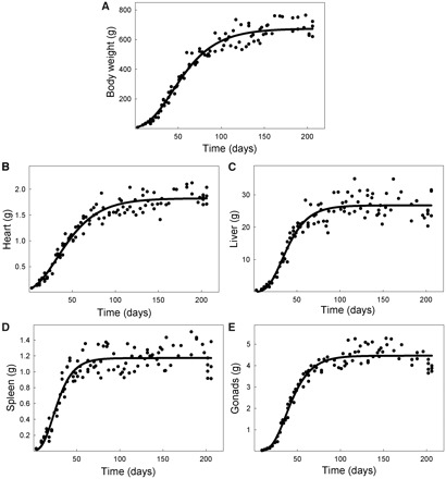
Growth trajectories of body and internal organs of male rats. Fitted curves are nonlinear Gompertz regressions. All plots use the same time axis. Parameters of the regressions are in Table 1. Data from Stewart and German (1999).
Table 1.
Parameters for Gompertz growth of various organs in male rats
| Organ | a | b | c | r 2 |
|---|---|---|---|---|
| Body | 675 | 4.58 | 0.035 | 0.965 |
| Heart | 1.82 | 3.44 | 0.038 | 0.939 |
| Liver | 26.7 | 7.22 | 0.061 | 0.907 |
| Spleen | 1.17 | 5.82 | 0.078 | 0.861 |
| Gonads | 4.46 | 9.70 | 0.062 | 0.959 |
We next used these growth parameters to derive the allometric curves using Equation (3). The allometries are shown in blue in Fig. 2 and in which we superimpose the calculated allometric curves over the raw data. In addition, we estimated the allometric parameters from the raw allometric data (using the nonlinear analysis tools in JMP-Pro 9.0.0; SAS Institute, Cary, NC, USA). The estimated curves are shown in red in Fig. 2 and the estimated parameter values are shown in Table 2. The allometries estimated by nonlinear regression closely fit those derived from the growth data, indicating that nonlinear regression methods can provide suitable estimates of the allometric relationships and of the underlying growth parameters. Figure 3 shows these allometries plotted on double logarithmic axes, which show that with one exception, the allometries are nonlinear, even after log-transformation.
Fig. 2.
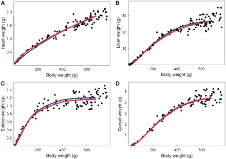
Ontogenetic allometries of body and internal organs in male rats based on the data in Fig. 1. Blue lines: Allometries derived from growth kinetics according to Equation (3b). Red lines: Allometries based on parameters estimated by nonlinear regression (Table 2).
Table 2.
Allometric parameters estimated from data on growth (Table 1), and estimated by nonlinear regression using Equation (3c) with t = tt.
| Allometry | Source | a | aa | b | bb | d |
|---|---|---|---|---|---|---|
| Body/heart | ||||||
| Growth | 675 | 1.82 | 4.58 | 3.44 | 1.07 | |
| Regression | 675 | 1.85 | 6.72 | 4.57 | 1.00 | |
| Body/liver | ||||||
| Growth | 675 | 26.7 | 4.58 | 5.82 | 1.72 | |
| Regression | 675 | 26.2 | 4.03 | 4.99 | 1.56 | |
| Body/spleen | ||||||
| Growth | 675 | 1.17 | 4.58 | 5.82 | 2.22 | |
| Regression | 670 | 1.15 | 3.53 | 2.75 | 2.06 | |
| Body/gonads | ||||||
| Growth | 675 | 4.46 | 4.58 | 9.70 | 1.67 | |
| Regression | 680 | 4.40 | 4.60 | 8.86 | 1.72 |
Fig. 3.
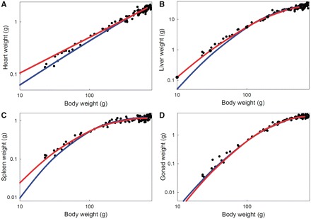
Double logarithmic plots of the allometries shown in Fig. 2.
Ontogenetic and static allometries
The allometries illustrated in Fig. 2 are ontogenetic allometries, because they follow the change in proportions over developmental time as the animal grows larger. Static allometries are allometric relationships among body parts at a given stage of development. In most studies, the stage of interest is the adult, but it could be any stage with definable characteristics. In mammals, this could be a stage such as birth, age at weaning, or age at first reproduction. In arthropods, the stage could be the hatchling, a specific larval stage, the pupa, or the adult.
Most studies use Huxley's equation to describe static allometry. Huxley's equation is derived from the growth kinetics of body parts and is an equation for ontogenetic allometry, so the implicit assumption is that static allometry is due to individual differences in the growth trajectory up to that stage in development. As, we argued above, Huxley's equation implicitly assumes that time is a free variable, so the implicit assumption of such studies is that static allometry is due to individual differences in the duration of growth until that stage.
In a system in which all parts grow simultaneously and continuously, as the one we explore here, it is difficult to define a “stage” based on morphometric traits. Even defining the adult stage is difficult, as rats become sexually mature at about 60 days, but continue to grow, albeit at an ever-decreasing rate, until well after 200 days. Two simple possibilities can be considered: A developmental stage could be equivalent to development time, or it could be the time at which a given organ, say the gonad, reaches a particular size. In either case, the static allometry would be the same as the ontogenetic allometry. Without an independent marker of stage, attempts to define a static allometry that is different from an ontogenetic allometry will be incorrect.
In some systems, a developmental stage can be defined in a way that is independent of development time or of the size of a particular structure. The adult stage of an insect is a good example. Adults do not grow or change form, and individual variation in the size and shape of adults is due to differences in the growth trajectories and the durations of growth of their various body parts. For instance, wings and bodies of holometabolous insects have independent growth trajectories and development times to a discrete final size that depends on both genetic and environmental factors (Nijhout and Grunert 2010). In such cases, the static allometry is not the same as the ontogenetic allometry. Instead, the static allometry can be deduced from individual differences in the growth trajectories and development times of the structures that are being compared. Such static allometries are the collection of endpoints of ontogenetic trajectories, and the equations that describe them do not resemble those of ontogenetic allometries (Nijhout and Wheeler 1996; Shingleton et al. 2008).
Phenotypic plasticity and allometry
There are two ways in which an environmental factor can alter an allometry. First, a factor such as temperature or nutrition could have a direct effect on the growth rate (or on the initiation or termination of growth), and this would alter both the ontogenetic and the static allometries among body parts. Second, an environmental factor can have an indirect effect by reprogramming development, for instance by altering the secretion of developmental hormones or growth factors or altering the expression of their receptors. Such effects can be tissue-specific. Good examples of this can be found in the allometries associated with insect polyphenisms, in which the relative growth of specific body parts is reprogrammed during metamorphosis and results in the disproportionate development of heads and appendages in ants (Feener et al. 1988; Wheeler 1991; Nijhout and Wheeler 1996), or in beetles’ horns (Emlen and Nijhout 2000; Moczek and Emlen 2000; Moczek and Nijhout 2002; Emlen and Allen 2003). Such plastic allometries (sensuSchlichting and Piggliucci [1998])are often nonlinear. The explanation for such nonlinearity in holometabolous insects is a bit more complicated than that outlined in the previous sections of this article, because the appendages of the adult begin their growth during metamorphosis, after the body has stopped growing (Nijhout and Emlen 1998; Nijhout and Grunert 2010). Thus, appendages grow in bodies of different sizes, and the size they attain is controlled by their growth rate in that environment (Nijhout and Wheeler 1996; Nijhout and Grunert 2010). In Manduca sexta, for instance, the wings grow slower and for a briefer period of time in a small body than in a large one (Nijhout and Grunert 2010), and limitation of the time available for growth has been implicated in the nonlinear wing-body scaling at large body sizes (Tobler and Nijhout 2010). The yearly growth of antlers in deer is another example of structures that grow in proportion to (a pre-existing) body size, and as deer grow larger from year to year, so do their new antlers (Schroder 1983; Weladji et al. 2005).
Linear and nonlinear allometries
Figure 4 shows a set of allometries that can be produced by Equation (3) using different sets of parameter values. Evidently, sigmoidal growth kinetics can produce quite diverse nonlinear allometries. Insofar, as growth trajectories are typically sigmoidal one would expect allometries to be fundamentally nonlinear. Note, however, that the size scale of variation in y in Fig. 4 ranges from 1 to 100. This is a large range that is typically only encountered in ontogenetic allometries. Static allometries usually deal with variation in size by a factor of 2 or less, and this would be represented by small segments of the curves in Fig. 4. Such small segments are often linear, or nearly so.
Fig. 4.
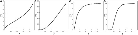
A set of nonlinear allometries (based on Equation [3b]) that can be produced by Gompertz growth. For simplicity, in all four plots, a and aa are fixed at 100, and t = tt. The other parameter values are (A) b = 30, bb = 8, c = 2, cc = 1; (B)b = 0.1, bb = 0.1, c = 1, cc = 1.2; (C) b = 2, bb = 0.5, c = 1, cc = 2.5; (D) b = 2, bb = 3, c = 0.5, cc = 2.
Two questions naturally arise from this observation. First, is the (near) linearity we typically find in static allometries accidental or does evolution favor combinations of growth parameters and body sizes that lead to (nearly) linear allometries? Second, how does one pick the right equation to fit to the observed data when the relationship looks nearly linear?
The first question suggests a new approach to studying the evolution of allometries. It seems reasonable to assume that natural selection would favor growth parameters that do not produce highly aberrant shapes at the extremes of a natural variation in body size, which implies that growth parameters and size ranges are likely to be selected to produce nearly linear allometries over the range of natural variation of size. It is an open question whether the severely nonlinear allometries one finds in many sexually selected traits (Emlen and Nijhout 2000) arose from the evolution of parameter values that produce just such an allometry, or whether they are more complex and require the reprogramming of growth kinetic parameters at certain body sizes (Wheeler 1991).
The answer to the second question depends rather on what kind of information one wishes to extract from the morphometric data. The study of allometry is often tackled as an exercise in curve fitting, and if the primary aim is to draw a well-fitting curve then one can use linear regression, or find the fit to a power equation or a polynomial equation and settle on the one that gives the largest coefficient of determination. Although such empirical equations allow one to compare allometries and determine if they differ statistically from one another, they are, unfortunately, biologically meaningless. If the aim is to understand the biology that gave rise to the allometry, or how differences in allometries are related to differences in the underlying growth patterns, or how the evolution of allometries is defined by (or constrained by) the evolution of growth patterns, then it is rather important to use biologically informative equations. The choice of equation then depends on the kinetics of growth and on the mechanism that causes variation in size. Most growth in biological systems is approximately Gompertz, so Equation (3) will generally be the most appropriate for ontogenetic allometries.
The evolution of allometries
One of the principal contributions that developmental biology can make to the study of evolution is to elucidate and explain the underlying mechanisms that give rise to traits, and thus provide the causal link between genotype and phenotype. Insofar as phenotypic evolution of morphology occurs primarily by changes in the sizes and proportions of body parts, understanding the developmental causes of size, variation in size, and proportional scaling helps us to understand how the evolution of form is due to the evolution of growth patterns. The study of scaling and allometry has had to rely on an inadequate causal mapping, and investigators have used a diversity of equations ranging from Huxley's power law to polynomials to “fit” scaling relationships without much concern for the underlying biology that gave rise to that relationship. We have shown here that allometric equations and the values of parameters can be derived from realistic sigmoid growth kinetics. Conversely, the underlying sigmoid-growth kinetic parameters can be deduced from the nonlinear allometry. In addition, this new set of allometric equations can be used to analyze what portions of a growth trajectory changed during evolution of the phenotype.
An example of how this could work is shown in Fig. 5. In Fig. 5A and D, we illustrate growth trajectories for a pair of structures, and the resulting allometric relationships. In Fig. 5B and E, we change one growth parameter, the damping exponent of structure yy, which causes it to reach its final size earlier than before and dramatically alters the shape of the allometry. In Fig. 5C and F, we change the growth exponent of structure y, which causes it to reach maximal size earlier than before with a very different effect on the shape of the allometry. Attempting to understand the evolution of these allometries by fitting and comparing polynomials, or by doing piecewise regressions on the inherently nonlinear data would likely yield rather convoluted explanations that obscure the fact that they come about by very simple changes in the growth kinetics of one of the structures. Here, understanding development is essential in understanding morphological evolution.
Fig. 5.
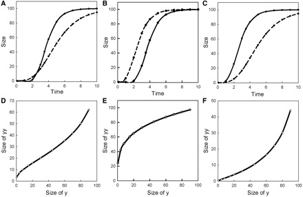
Growth trajectories of two structures, y (solid line) and yy (dashed line), growing with Gompertz kinetics (A, B, C) and the resulting allometric relationships among them (D, E, F). For simplicity, in all plots, a and aa are fixed at 100, and t = tt. The other parameter values are (A and D) b = 30, bb = 8, c = 2, cc = 1; (B and E) as in (A) except cc = 2; (C and F) as in (A) except b = 10.
Funding
This work was supported by grants IOS-0744952 and EF-1038593 from the National Science Foundation.
Acknowledgments
We thank Viviane Callier, Inder Jalli, Rick Dilling, and two anonymous reviewers for constructive critical comments.
References
- Edelstein-Keshet L. Mathematical models in biology. New York: Random House; 2005. [Google Scholar]
- Emlen DJ. Artificial selection on horn length-body size allometry in the horned beetle Onthophagus acuminatus (Coleoptera: Scarabaeidae) Evolution. 1996;50:1219–30. doi: 10.1111/j.1558-5646.1996.tb02362.x. [DOI] [PubMed] [Google Scholar]
- Emlen DJ, Allen CE. Genotype to phenotype: Physiological control of trait size and scaling in insects. Integr Comp Biol. 2003;43:617–34. doi: 10.1093/icb/43.5.617. [DOI] [PubMed] [Google Scholar]
- Emlen DJ, Nijhout HF. Hormonal control of male horn length dimorphism in the dung beetle Onthophagus taurus (Coleoptera : Scarabaeidae) J Insect Physiol. 1999;45:45–53. doi: 10.1016/s0022-1910(98)00096-1. [DOI] [PubMed] [Google Scholar]
- Emlen DJ, Nijhout HF. The development and evolution of exaggerated morphologies in insects. Annu Rev Entomol. 2000;5:661–708. doi: 10.1146/annurev.ento.45.1.661. [DOI] [PubMed] [Google Scholar]
- Emlen DJ, Nijhout HF. Hormonal control of male horn length dimorphism in Onthophagus taurus (Coleoptera: Scarabaeidae): a second critical period of sensitivity to juvenile hormone. J Insect Physiol. 2001;47:1045–54. doi: 10.1016/s0022-1910(01)00084-1. [DOI] [PubMed] [Google Scholar]
- Falconer DS, Mackay TFC. Introduction to quantitative genetics. Harlow: Addison Wesley Longman; 1996. [Google Scholar]
- Feener DH, Jr, Lighton JRB, Bartholomew GA. Curvilinear allometry, energetics and foraging ecology: a comparison of leaf-cutting ants and army ants. Funct Ecol. 1988;2:509–20. [Google Scholar]
- Gayon J. History of the concept of allometry. Am Zool. 2000;40:748–58. [Google Scholar]
- German RZ, Meyers LL. The role of size and time in ontogenetic allometry: II. An empirical study of human growth. Growth Dev Aging. 1989;53:107–15. [PubMed] [Google Scholar]
- Huxley JS. Problems of relative growth. London: Methuen; 1932. [Google Scholar]
- Huxley JS, Teissier G. Terminology of relative growth rates. Nature. 1936;137:780–1. [Google Scholar]
- LaBarbera M. Analyzing body size as a factor in ecology and evolution. Annu Rev Ecol Syst. 1989;20:97–117. [Google Scholar]
- Laird AK. Dynamics of tumor growth. Br J Cancer. 1964;18:490–502. doi: 10.1038/bjc.1964.55. [DOI] [PMC free article] [PubMed] [Google Scholar]
- Lammers AR, German RZ. Ontogenetic allometry in the locomotor skeleton of specialized half-bounding mammals. J Zool. 2002;258:485–95. [Google Scholar]
- Miller JP, German RZ. Protein malnutrition affects the growth trajectories of the craniofacial skeleton in rats. J Nutr. 1999;129:2061–9. doi: 10.1093/jn/129.11.2061. [DOI] [PubMed] [Google Scholar]
- Moczek AP. Allometric plasticity in a polyphenic beetle. Ecol Entomol. 2002;27:58–67. [Google Scholar]
- Moczek AP, Emlen DJ. Male horn dimorphism in the scarab beetle, Onthophagus taurus: do alternative reproductive tactics favour alternative phenotypes? Anim Behav. 2000;59:459–66. doi: 10.1006/anbe.1999.1342. [DOI] [PubMed] [Google Scholar]
- Moczek AP, Nijhout HF. Developmental mechanisms of threshold evolution in a polyphenic beetle. Evol Dev. 2002;4:252–64. doi: 10.1046/j.1525-142x.2002.02014.x. [DOI] [PubMed] [Google Scholar]
- Moczek AP, Nijhout HF. Rapid evolution of a polyphenic threshold. Evol Dev. 2003;5:259–268. doi: 10.1046/j.1525-142x.2003.03033.x. [DOI] [PubMed] [Google Scholar]
- Nijhout HF. Development and evolution of adaptive polyphenisms. Evol Dev. 2003;5:9–18. doi: 10.1046/j.1525-142x.2003.03003.x. [DOI] [PubMed] [Google Scholar]
- Nijhout HF. Dependence of morphometric allometries on the growth kinetics of body parts. J Theor Biol. 2011;288:35–43. doi: 10.1016/j.jtbi.2011.08.008. [DOI] [PubMed] [Google Scholar]
- Nijhout HF, Emlen DJ. Competition among body parts in the development and evolution of insect morphology. Proc Natl Acad Sci USA. 1998;95:3685–9. doi: 10.1073/pnas.95.7.3685. [DOI] [PMC free article] [PubMed] [Google Scholar]
- Nijhout HF, Grunert LW. The cellular and physiological mechanism of wing-body scaling in Manduca sexta. Science. 2010;330:1693–5. doi: 10.1126/science.1197292. [DOI] [PubMed] [Google Scholar]
- Nijhout HF, Wheeler DE. Growth models of complex allometries in holometabolous insects. Am Nat. 1996;148:40–56. [Google Scholar]
- Reichling TD, German RZ. Bones, muscles and visceral organs of protein-malnourished rats (Rattus norvegicus) grow more slowly but for longer durations to reach normal final size. J Nutr. 2000;130:2326–32. doi: 10.1093/jn/130.9.2326. [DOI] [PubMed] [Google Scholar]
- Schlichting CD, Pigliucci M. Phenotypic evolution: a reaction norm perspective. Sunderland (MA): Sinauer Inc; 1998. [Google Scholar]
- Schroder J. Antler and body weight allometry in red deer: a comparison of statistical estimators. J Biometr. 1983;25:669–80. [Google Scholar]
- Shingleton AW, Mirth CK, Bates PW. Developmental model of static allometry in holometabolous insects. Proc R Soc Biol Sci Ser B. 2008;275:1875–85. doi: 10.1098/rspb.2008.0227. [DOI] [PMC free article] [PubMed] [Google Scholar]
- Shingleton AW, Estep CM, Driscoll MV, Dworkin I. Many ways to be small: different environmental regulators of size generate distinct scaling relationships in Drosophila melanogaster. Proc R Soc B Biol Sci. 2009;276:2625–33. doi: 10.1098/rspb.2008.1796. [DOI] [PMC free article] [PubMed] [Google Scholar]
- Stewart SA, German RZ. Sexual dimorphism and ontogenetic allometry of soft tissues in Rattus norvegicus. J Morphol. 1999;242:57–66. doi: 10.1002/(SICI)1097-4687(199910)242:1<57::AID-JMOR4>3.0.CO;2-5. [DOI] [PubMed] [Google Scholar]
- Tobler A, Nijhout HF. Developmental constraints on the evolution of wing-body allometry in Manduca sexta. Evol Dev. 2010;12:592–600. doi: 10.1111/j.1525-142X.2010.00444.x. [DOI] [PubMed] [Google Scholar]
- Verhulst P. Notice sur la loi que la population suit dans son accroissement. Corr Math Phys. 1838;10:113–7. [Google Scholar]
- Weladji R, Holand Ø, Steinheim G, Colman J, Gjøstein H, Kosmo A. Sexual dimorphism and intercorhort variation in reindeer calf antler length is associated with density and weather. Oecologia. 2005;145:549–55. doi: 10.1007/s00442-005-0155-8. [DOI] [PubMed] [Google Scholar]
- Wheeler DE. The developmental basis of worker caste polymorphism in ants. Am Nat. 1991;138:1218–38. [Google Scholar]
- White JF, Gould SJ. Interpretation of the coefficient in the allometric equation. Am Nat. 1965;99:5. [Google Scholar]
- Wilson E. The insect societies. Cambridge: Harvard University Press; 1971. [Google Scholar]