

Abstract
The blood-oxygen-level-dependent (BOLD) signal in functional MRI (fMRI) measures neuronal activation indirectly. Previous studies have found aperiodic, systemic low-frequency oscillations (sLFOs, ~0.1Hz) in BOLD signals from resting-state (RS) fMRI, which reflects the non-neuronal cerebral perfusion information. In this study, we investigated the possibility of extracting vascular information from the sLFOs in RS BOLD fMRI, which could provide complementary information to the neuronal activations. Two features of BOLD signals were exploited. First, time delays between the sLFOs of big blood vessels and brain voxels were calculated to determine cerebral circulation times and blood arrival times. Second, voxel-wise standard deviations (SD) of LFOs were calculated to represent the blood densities. We explored those features on the publicly available Myconnectome dataset (a two-year study of an individual subject (Male)), which contains 45 RS scans acquired after the subject had coffee, and 45 coffee-free RS scans, acquired on different days. Our results showed that shorter time delays and smaller SDs were detected in caffeinated scans. This is consistent with the vasoconstriction effects of caffeine, which leads to increased blood flow velocity. We also compared our results with previous findings on neuronal networks from the same dataset. Our finding showed that brain regions with the significant vascular effect of caffeine coincide with those with significant neuronal effect, indicating close interaction. This study provides methods to assess the physiological information from RS fMRI. Together with the neuronal information, we can study simultaneously the underlying correlations and interactions between vascular and neuronal networks, especially in pharmacological studies.
Keywords: Magnetic resonance imaging, cerebral blood flow, cerebral cortex, blood vessels
Graphical Abstract
The fMRI BOLD signals were influenced by the vasoconstriction effects of caffeine. The vasoconstriction effects of caffeine decreased the vascular density (small standard deviations) and increased the speed of blood flow (short time delays).
1. Introduction
Blood-oxygen-level-dependent (BOLD) contrast in functional magnetic resonance imaging (fMRI) has been widely applied to investigate brain activity (Bandettini et al. 1992; Ogawa et al. 1992). However, BOLD fMRI does not measure neuronal activation directly. It reflects neuronal activation through the neurovascular coupling. In addition to neuronal activity, physiological processes which make alterations in cerebral blood flow (CBF), cerebral blood volume (CBV) and cerebral blood oxygen consumption (CMRO2) can also affect BOLD signals (Buxton et al. 2004; D’Esposito et al. 2003; Hoge et al. 1999). Thus, some features of BOLD signals can be used to assess systemic physiology. This additional physiological information does not require extra scans. More importantly, it can offer concurrent and complement physiological information to the neuronal activation. The combined information can shed light on the interactions between neuronal activation and non-neuronal physiological processes.
Among all the features of resting-state (RS) BOLD signals, it has been demonstrated that the time delay and amplitude of low-frequency fluctuations (ALFFs) can be used to assess the cerebral blood velocity and cerebral blood density respectively (Tong 2010; Vigneau-Roy et al. 2014). Systemic low-frequency oscillations (sLFOs) are the physiological RS BOLD signals with the frequency range from 0.01 to 0.1Hz, which overlaps with the frequency range of RS BOLD signals (i.e. neuronal). However, the RS BOLD signals are more regional, leading to different RS networks with corresponding RS BOLD signals. On the other hand, sLFOs were traveling global signals with likely extracerebral origins (Hocke et al. 2016), which might be related to CO2 fluctuation in the blood, vasomotion, Mayer wave, etc (Golestani et al. 2016; Julien 2006; Wise et al. 2004). The reason that they are called “systemic” is that the same sLFOs, which are found in RS BOLD signals in the brain (especially large veins), can be detected concurrently by optical method at peripheral sites (fingertip and toe) as slow changes in oxy- and deoxyhemoglobin concentration with time delays (Tong et al. 2013). This study demonstrated that the sLFO is a blood-borne oscillation which travels to different parts of the body with blood. Recently, we were able to identify these sLFOs in large arteries and veins (i.e. the internal carotid artery (ICA), superior sagittal sinus (SSS) and internal jugular vein) in the neck from the resting state (RS) Myconnectome data (Tong et al. 2018). Time delays of approximately 7 seconds were found between these two highly correlated signals, which is consistent with the cerebral circulation time (CCT) normally measured by ultrasound (Strangman et al. 2002). Another feature is ALFFs (ALFF was determined by standard deviation (SD) of LFO time series), which also provides physiological cerebral vascular properties, such as cerebral blood volume, vascular density, etc (Yan et al. 2011). The ALFFs has been shown to contain a vascular component related to hypercapnic index (Kannurpatti et al. 2008). Vigneau-Roy et al. 2014 illustrated that the ALFFs of RS BOLD signals were related to vascular density (Vigneau-Roy et al. 2014). The LFO amplitude has also been used to indicate vasoconstriction (Rack-Gomer et al. 2009).
In this study, we exploited these parameters to derive the non-neuronal physiological parameters from RS fMRI studies and combine the results with the neuronal findings.
Caffeine, as an adenosine A2 receptor antagonist, has both neuronal and cerebral vascular effect. For neuronal effects, it is well-known that caffeine can increase the alertness level (Hindmarch et al. 2000). It has also been found that visual BOLD response is faster after ingestion of caffeine (Behzadi and Liu 2006; Liau et al. 2008; Liu et al. 2004). Many studies on caffeine effects in the brain focus on these neuronal activities, e.g. investigating brain network connectivity (Rack-Gomer et al. 2009; Tal et al. 2013; Wu et al. 2014). However, caffeine also has profound vascular effects. After 250 mg caffeine intake, the resulting vasoconstriction can decrease the CBF about 27% (Addicott et al. 2009; Griffeth et al. 2011; Mathew and Wilson 1985). These global vascular effects also alter RS BOLD signals as we discussed previously. So far, few fMRI studies have sought to understand caffeine’s vascular effect on RS fMRI, and more importantly, understand the interaction with neuronal activations. In this work, we will study vascular effects of caffeine using 1) time delays between sLFOs to map cerebral circulation time and cerebral blood arrival; 2) LFOs’ SDs to infer the blood density or the size of large cerebral blood vessel. The results will be compared with those from brain network analyses (published separately) and paint a thorough picture of the effects of caffeine.
2. Method
2.1. Data selection
The publicly available Myconnectome dataset (http://myconnectome.org/wp) was chosen to investigate the cerebral vascular effects of caffeine. This dataset is about a two-year study of an individual subject (Male, aged 45). We included the RS scans from session 13 to session 104 (no RS scan in session 52 and session 90), and excluded the pilot sessions and follow-up sessions. There are a number of advantages to using this dataset: (1) the Myconnectome dataset recruited only one single subject, which eliminates between-subject variation. (2) The data contains 90 high-quality resting-state fMRI scans, with the equal number of caffeinated scans (scans were taken 90 minutes after caffeine ingestion) and un-caffeinated scans (i.e. 45 each). (3) Structural images included T1 and T2 weighted scans with high spatial resolution, which made identification of large blood vessels (arteries and veins) easier.
2.2. Image acquisition
Detailed scan parameters can be found in Poldrack et. al 2015. In short, most of the 10 minute resting-state fMRI scans with eyes closed were acquired using multi-band EPI sequence (TR=1.16 s, TE=30 ms, flip angle=63 degrees (the Ernst angle for grey matter), voxel size=2.4 × 2.4 × 2 mm, distance factor=20(percentage sign), 68 slices, oriented 30 degrees back from AC/PC, 96 × 96 matrix, 230 mm FOV, MB factor=4, 10:00 scan length) (Poldrack et al. 2015).
2.3. Data processing
Figure 1 shows the flow chart of data processing. Data were processed using FSL (FMRIB Expert Analysis Tool, v6.01, http://www.fmrib.ox.ac.uk/fsl, Oxford University, UK (Jenkinson et al. 2012)) and a locally developed Matlab program (MATLAB 2017a, The MathWorks Inc., Natick, MA, 2000). RS fMRI scans were preprocessed with following steps recommended by Power et al., 2014. This included: 1) motion correction (FSL mcflirt), 2) linear detrending (MATLAB detrend; ‘linear’), 3) Nuisance signals removal (six motion parameters and their derivatives estimated by mcflirt) using general linear model (FSL fsl_glm), 4) spatial smoothing with a Full-Width Half-Maximum of 5mm isotropic Gaussian kernel (Power et al. 2014).
Figure 1.

The flowchart presents the procedure of data processing. First, ninety resting-state scans were sorted into caffeinated and uncaffeinated groups. Second, vascular information was extracted from scans separately, which included 1) Time delays between systemic low-frequency oscillations (sLFOs, 0.01Hz-0.1Hz) of superior sagittal sinus (SSS) and brain voxels, 2) Cerebral circulation time (CCT) was measured by time delay between sLFOs of SSS and internal carotid artery (ICA), 3) LFOs amplitude in brain voxels were measured. Lastly, the above vascular effect of caffeine was compared with the neuronal effect of caffeine from previous research.
2.4. Vascular measures
We assessed the caffeinated/uncaffeinated difference in the following parameters: 1) CCT from the time delays between sLFOs in fMRI signals from ICA and SSS; 2) delay maps (i.e. cerebral blood arrival map) obtained by calculating the voxel-wise time delays between sLFOs in fMRI signals from each voxel and SSS; 3) cerebral blood density from the voxel-wise SDs (ALFFs) of LFO in fMRI signals. Lastly, we compared our results with previous research of RS networks connectivity on the same dataset. (Poldrack et al. 2015)
2.4.1. Cerebral circulation
In order to calculate the delays of the sLFOs between ICA and SSS in caffeinated and uncaffeinated scans, we applied the same method in Tong et al. 2018 to extract the fMRI signals in these large blood vessels. In short, left and right ICAs and SSS were identified from structural images (T1- and T2- weighted images) (Tong et al. 2018). Time series within these identified blood vessels were extracted and averaged (FSL fslmeants) from the resting state fMRI (after registering high-resolution vessel masks onto the low-resolution fMRI images). To calculate the time delays between the sLFOs of two vessels, we conducted the following steps. 1) A band-pass zero-lag Butterworth filter (0.01-0.1Hz) was applied to the time series from SSS, global signal (GS) and ICA to extract the sLFOs, which were then oversampled to increase the temporal resolution (from 1.16s to 0.116 s). 2) The principal component analysis was then applied on the signals from left and right ICAs to obtain the principal signal of the low-frequency component to improve the signal-to-noise ratio. 3) Time delays between the sLFOs from GS, ICA, and SSS were calculated using cross-correlation (xcorr in Matlab), which found the absolute maximum cross-correlation coefficient (MCCC) between the signals within a ±15s window. The MCCC threshold was set at 0.28, which was the significance threshold based on previous research (Hocke et al. 2016). In addition, voxel-wise delay maps were generated based on the method developed previously (Tong and Frederick 2014). In short, the time delay between every voxel’s RS BOLD signal and the SSS signal was calculated to represent the blood arrival time at that voxel. The delays calculated between large vessels, as well as the whole brain delay maps, were later compared between caffeinated and uncaffeinated scans to expose the caffeine effects on the circulation.
2.4.2. Cerebral blood density (volume)
Previous research reported that the ALFFs in the RS BOLD signal were positively correlated with blood density in the voxel (Vigneau-Roy et al. 2014). Here, we calculated the SD in RS BOLD signal to represent the cerebral blood density (volume). Voxel-wise SD maps were calculated with the following steps: First, a band-pass zero-lag Butterworth filter (0.01-0.1Hz) was applied to the time series of each voxel in the brain. Second, SDs of the low-frequency time series were calculated in each voxel. Finally, the SD differences (in percentage) between caffeinated and uncaffeinated scans were obtained by the subtraction.
2.4.3. Statistical analysis
The distributions differences of time delays between GS, ICA, and SSS in caffeinated and uncaffeinated scans were tested by the Kolmogorov—Smirnov test (Daniel 1990).
To assess the statistical significance of the difference between caffeinated and uncaffeinated scans, we conducted the randomization procedure. In detail, 90 delay maps (or SD maps) were randomly placed into two groups (45 each). Each group would have roughly same numbers of caffeinated scans as well as uncaffeinated scans. The averaged delay maps (or SD maps) were calculated from each group and the subtraction between these two groups was obtained. Since there is no difference in the subtraction (because equal numbers of caffeinated and uncaffeinated scans are included in each group), the subtraction result should be close to 0 and its distribution could be used to extract the threshold of the null hypothesis to assess the real effect. The processes of generating random groups and the subtraction between these groups were repeated for 10000 trials. The threshold was selected as P < 0.01 or P > 0.99 (P indicated the probability of having spurious results), from the averaged distribution of the subtractions. Also, we applied two-sample t-test to further validate the differences in the delay and SD maps between caffeinated and uncaffeinated scans (SPM (https://www.fil.ion.ucl.ac.uk/spm/)). The resulting SPM[T] map was thresholded at p < 0.05, corrected for multiple comparisons using the false discovery rate (FDR)-criterion (Genovese et al. 2002).
3. Results
3.1. Comparison of caffeinated and uncaffeinated results
3.1.1. Cerebral circulation time (CCT) difference
Figure 2 shows the time delay differences between SSS and GS, GS and ICA, ICA and GS. Time delays are significantly shorter between SSS and ICA in the caffeinated scans (5.03±0.617s) than those from the uncaffeinated scans (5.96±0.659s) (p < 0.001), indicating the shorter CCTs in caffeinated scans. This result is consistent with the following observations: 1) time delays are significantly shorter between SSS and GS in the caffeinated scans (2.15±0.237s) than the uncaffeinated scans (2.74±0.303s) (p < 0.001). 2) time delays are significantly shorter between GS and ICA in caffeinated scans (2.87±0.767s) than uncaffeinated scans (3.38±0.783s) (p < 0.05);
Figure 2.
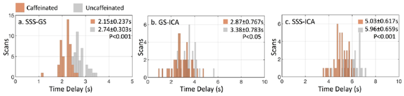
Comparison of time delay distribution between 45 caffeinated RS scans (brown) and 45 uncaffeinated RS scans (gray). Time delays were calculated between (a) SSS and GS, (b) GS and ICA and (c) SSS and ICA. Results with absolute maximum cross-correlation coefficient less than 0.28 were excluded to avoid spurious correlations. Time delay distributions between caffeinated and uncaffeinated scans were compared by Kolmogorov-Smirnov test.
3.1.2. Delay map difference
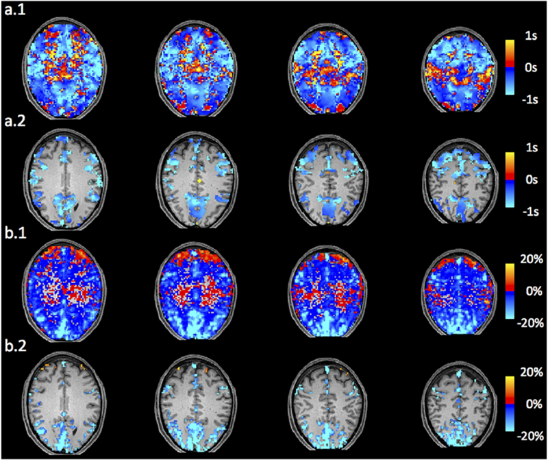
Figure 3.a shows the average delay map from 90 RS scans (from a single subject). It demonstrates that the delay map calculated from this data largely matches the cerebral blood circulation. Red indicates the early arrival of the sLFOs (i.e. blood), while blue denotes late arrival. Since the voxel-wise delay value was calculated between the sLFO from each voxel and the SSS, the arrival times were relevant to that of SSS. Figure 3.a shows that the brain is dominated by “Red”, indicating that blood reached most of the voxels before it arrived at SSS (which is expected, as the SSS is a major blood drainage vessel from the brain). Interestingly, the ICAs were automatically identified as the regions where blood arrives very early (see the arrows in Figure 3.a). This phenomenon confirmed that sLFOs indeed were “pumped” into the brain through arteries, such as ICAs. The detailed discussion about the sLFOs in ICA can be found in our previous publication (Tong et al. 2018). The fact that the delay map can automatically locate ICA out of RS fMRI data with correct delay values showed the robustness of the sLFO in fMRI signal as well as our method. Delay map difference obtained by subtracting the delay map of 45 caffeinated scans from that of 45 uncaffeinated scans is shown in Figure 3.b. It shows that the subtracting result of the delay maps is dominated by “Blue”, indicating that blood flow speed increased in most of the brain regions under the effect of caffeine.
Figure 3.

(a) Averaged delay map from 90 RS scans. Time delays were calculated between sLFOs of SSS and all the voxels in the brain. The red-yellow color showed later arrival time of blood and blue color showed earlier arrival time with reference to SSS. (b) The difference between caffeinated and uncaffeinated delay maps. Blue-lightblue color showed time delays between the voxels and SSS were shorter in the caffeinated scans than the uncaffeinated scans.
Figure 4.a shows the distribution of randomized subtraction (from 10000 random combinations) in blue and the that of real caffeinated vs. uncaffeinated subtraction in red (see 2.4.3). From the distribution of randomized subtraction in Figure 4.a, we found the results were clustered tightly around 0, which was expected due to no caffeine effects in the randomized data. However, the distribution of real caffeinated vs. uncaffeinated subtraction was much broader. This further indicates that the differences calculated between caffeinated and uncaffeinated scans are significant. We obtained the thresholds on delay differences to be > 0.037s or < −0.042s (P < 0.01), which were used on Figure 5.a.1 and upper panel of Figure 8 to produce statistically significant delay maps differences. Also, Figure 5.a.2 showed that the delay differences between caffeinated and uncaffeinated scans were significant (i.e. two-sample t-test) at a low statistical threshold (p < 0.05, FDR corrected).
Figure 4.
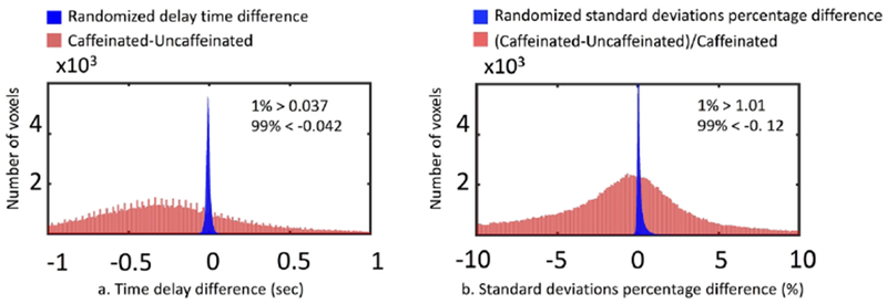
Original results of time delay difference (a) and SD difference (b) between caffeinated and uncaffeinated scans were presented as red distribution. Randomization results of time delay difference (a) and SD difference (b) between caffeinated and uncaffeinated scans were presented as blue distribution.
Figure 5.
(a.1) Randomization corrected subtraction of delay map (caffeinated-uncaffeinated) . (a.2) Subtraction of delay map corrected by FDR (p<0.05) (caffeinated-uncaffeinated). (b.1) SD percentage difference ((caffeinated-uncaffeinated)/caffeinated). (b.2) Randomization corrected SD percentage difference corrected by FDR (p<0.05) ((caffeinated-uncaffeinated)/caffeinated).
Figure 8.
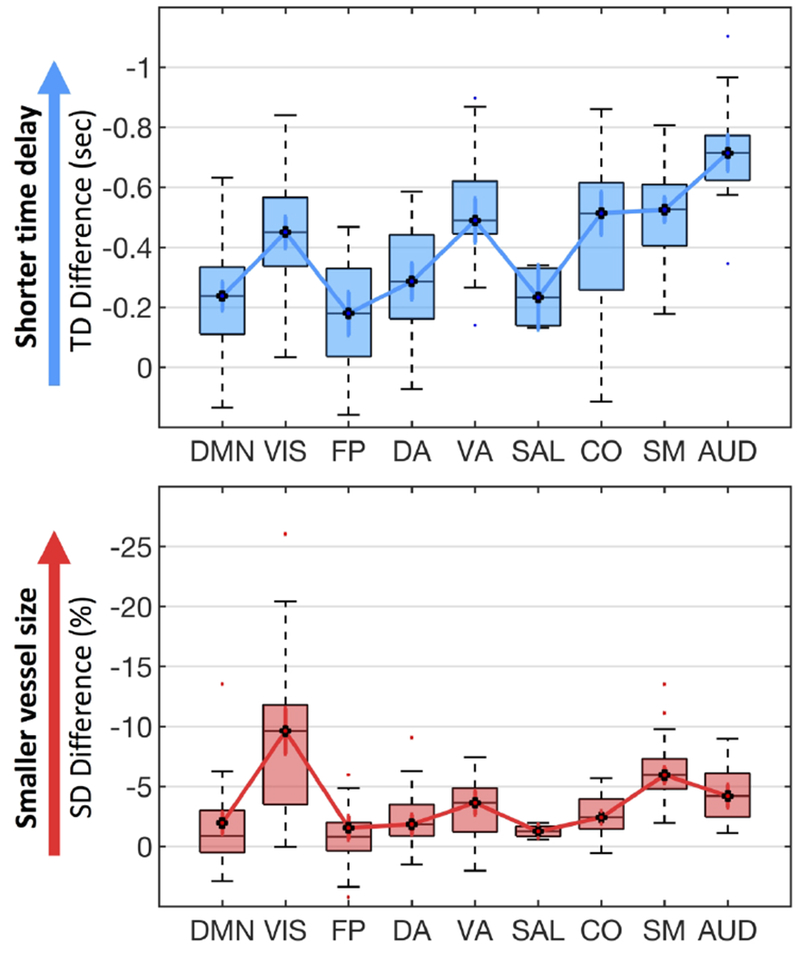
Vascular effect of caffeine on 9 RS networks. The significant time delay differences (upper blue panel) and SD differences (lower red panel) between caffeinated and uncaffeinated scans were showed for 9 RS networks. (DMN: default mode network, VIS: visual network, FP: fronto-parietal network, DA: dorsal attention network, VA: ventral attention network, SAL: salience network, CO: cingulo-opercular network, SM: somatomotor network, AUD: auditory network).
3.1.3. Standard deviation difference
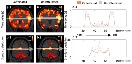
Figure 6.a shows that voxels with higher LFO amplitude (i.e. SD) in yellow, projected onto the subject’s own structural scan (T2-weighted image). The yellow regions overlapped precisely with the visible blood vessels (marked by squares in T2-weighted image Figure 6.b). This is in accordance with the findings in Vigneau-Roy et al. 2014, which reported that the ALFFs of RS BOLD signal were positively correlated with blood density in the voxel (Vigneau-Roy et al. 2014). We used this feature to assess blood vessel changes due to caffeine effect. The rows/columns of voxels (shown by arrows) in Figure 7.a(1-2) pass through areas with high blood density (or large blood vessels). The corresponding profile (of RS BOLD signals’ SDs along the white arrow) is shown in Figure 7.b(1-2), which presented the averaged results of uncaffeinated scans and caffeinated scans. From Figure 7.a(1-2), visible decreases in the yellow pattern were found in caffeinated results, which is confirmed by Figure 7.b(1-2). It shows the intensity profile of the SDs of LFOs was “constricted” and decreased after coffee. This observation could be interpreted as vasoconstriction due to the caffeine. To assess the vessel constriction effect in the whole brain, we compared the SD difference in percentage ((caffeinate – uncaffeinated)/(caffeinated)) between caffeinated and uncaffeinated scans. To assess the result in the statistical point of view, we also conducted the “randomization” procedure used before, with similar findings (shown in Figure 4.b). The distribution of real caffeinated vs. uncaffeinated subtraction was much broader than the results from randomized subtractions, indicating the difference calculated between caffeinated vs. uncaffeinated is not spurious but robust. We obtained the thresholds on percentage SD difference to be > 1.01% or < −0.12% (P < 0.01), which were applied on Figure 5.b.1 and lower panel of Figure 8 to produce the map of statistically significant SD differences. Also, Figure 5.b.2 showed that the SD differences between caffeinated and uncaffeinated scans were significant (i.e. two-sample t-test) at a low statistical threshold (p < 0.05, FDR corrected).
Figure 6.
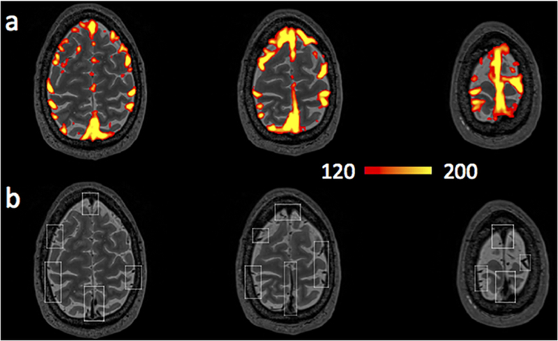
(a) Averaged SD map from 90 RS scans. (b) T2-weighted image. Brain region with high sLFO amplitude matched the locations of big blood vessels (marked by squares in (b)).
Figure 7.
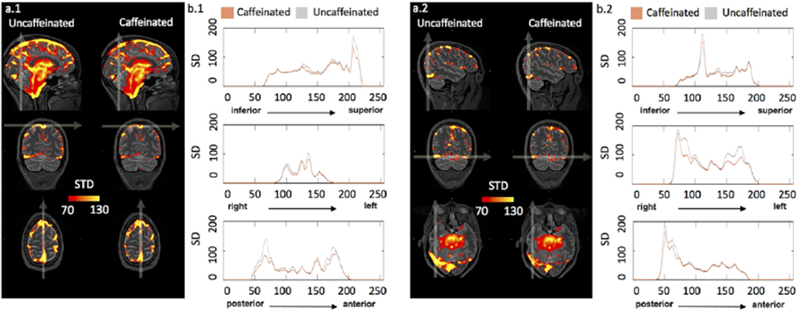
(a1-2) show the average SD maps of caffeinated and uncaffeinated scans at different MNI coordinates. (b1-2) were SD intensity profiles, which reflected the corresponding SD values along the white arrow in both averaged uncaffeinated (gray) and caffeinated scans (brown) from (a1-2),respectively.
3.2. Neuronal and vascular effects
As we know, caffeine has both vascular and neural effects. It is of great interest to understand the spatial correlation between vascular and neuronal effect (from previous studies). In detail, we conducted following steps: First, significant whole brain time delay differences (Figure 5.a) and SD percentage differences (Figure 5.b) were parcellated according to nine functionally coherent RS networks (Gordon et al. 2014). These well-known RS networks have been studied with the Myconnectome dataset previously to assess the neuronal effect of caffeine (Laumann et al. 2015; Poldrack et al. 2015). Subsequently, the average of time delay differences and SD percentage differences were obtained from each network. The results were showed in Figure 8. Negative values of blue boxplot indicated shorter time delays, while negative values of red boxplot showed smaller vessel size after caffeine intake.
In Figure 8, significantly shorter time delays and smaller SDs can be found in all nine RS networks in caffeinated scans. Top four RS networks with the highest time delay differences (i.e. auditory, somatomotor, visual and, ventral attention networks), are also the top four networks with the highest SD percentage differences. Moreover, we found high linear correlation between relative fluctuations (represented by black dotted linked by solid lines in Figure 8.) in averaged differences of time delays and SDs among different networks (r= 0.6, p= 0.09, high p-value reflected few data points). This feature indicates that network-specific flow velocity changes well correlated with the vessel size changes under the influence of caffeine.
Interestingly, Poldrack et al. found significantly lower connectivity within and between somatomotor, dorsal attention and visual networks in caffeinated scans. Moreover, similar decreasing connectivity was found within motor cortex after caffeine intake (Rack-Gomer et al. 2009). These RS networks (i.e. motor, visual) with decreasing connectivity were the same networks which have the largest time delays and SDs changes after caffeine intake (except dorsal attention network). It shows that caffeine has profound vascular effects (e.g. vessel constriction) in the brain regions where neuronal connectivities were also weakened. This is the first study to expose simultaneously the vascular and neuronal effect of a drug from the same resting state fMRI data. The interaction between regional perfusion and neuronal activity, exposed by the method, are crucial for the understanding of the effects of drugs, brain diseases, etc. More qualitative studies large populations are needed to fully explore the effects.
4. Discussion
4.1. Caffeinated scans have the faster speed of blood flow
Figure 2 showed statistically significant shorter time delays of sLFOs between SSS and ICA, in caffeinated scans than in uncaffeinated scans (~0.9s), which could be interpreted as decreases of CCTs. However, studies from positron emission tomography (PET) and arterial spin labeling (ASL) reported that decreasing CBF was detected after caffeine ingestion (Addicott et al. 2009; Cameron et al. 1990; Rack-Gomer et al. 2009; Wong et al. 2012). Decreasing CBF would, on the surface, seem to imply an increase of the CCT. This seems to contradict the finding in this study. One possible explanation may lay in the fact that CCT is not necessarily inversely correlated with CBF. CCT reflects the time for a bolus or red blood cells to travel from the ICA to the SSS (speed). However, CBF is measured in the amount of blood (ml) passing through a certain mass of tissue (100g) in unit time (e.g. min). If vessel size stays the same, an increase in CBF will decrease CCT. However, in the situation of caffeine, pressure induced by vessels constriction (coupled with elevated cerebral blood (James 2004)) leads to the increased blood flow speed (see section 4.2 in the discussion). However, the effects of vessel constriction on CBF are twofold: 1) elevated blood speed will increase CBF; 2) vessel constriction will decrease CBF. Since the latter effect is dominant (~r2, r is vessel diameter), vessel constriction will lead to a decrease in CBF. This model explains how caffeine related vessel constriction can increase the blood flow speed inside the vessels, (leading to shorter CCT) while decreasing the CBF. Nevertheless, caffeinated study using transcranial Doppler to measure the velocity of the middle cerebral artery (MCA) after 250mg of caffeine ingestion showed the significant reduction of the velocity by 13% and reduction of MCA diameter by 4.3% (Lunt et al. 2004). This does not contradict our model (see in next paragraph) since the RS BOLD signals we studied (e.g. SSS and global mean) are mostly vein signals. The perfusion parameters we derived, including time delay and SD, are biased/more sensitive towards the venules and veins. Therefore, we think the velocity change and vessel constriction measured by RS BOLD signals mostly happens in the capillary, venules, and veins (see discussion in 4.3).
Delay map differences between uncaffeinated scans and caffeinated scans are shown in Figure 5.a. The regions in red are the areas where the time delays are shortened referred to SSS (i.e. increase cerebral blood flow speed). Figure 5.a showed that in most of the brain the cerebral blood flow speed did increase mildly (within 1s) after caffeine intake. However, there are also regions where cerebral blood flow speed reduced (blue regions: longer time delays referred to SSS, especially in Figure 5.a). These regions are concentrated in the lower part of the brain overlapping with MCA. This observation matched the previous publication of transcranial doppler studies of caffeine (Lunt et al. 2004).
4.2. Caffeinated scans have lower LFO amplitude
It has been known that areas of high SDs in RS fMRI correspond very well with large vessels in the flow-weighted image (Kim et al. 1994). It was even suggested to use these SD maps to identify the location of large vessels. A recent study has investigated the link between regional variations of vascular density (VAD) and the ALFFs of RS BOLD signals. They found the positive correlation between the VAD (from the venous vascular tree in susceptibility-weighted imaging) and the ALFFs. These findings were similar to the results showed in Figure 6. As result, vessel constriction will decrease the VAD signal, which results in smaller ALFFs. We can see in Figure 7 that the SD profile curves are narrower and shorter in the caffeinated scans, which indicated that the effect of caffeine is largely vessel constriction. This is more obvious in the case of large veins. In the top left graphs of Figure 7, SSS were identified with RS BOLD signals of high SD. Its diameter became smaller after caffeine intake. The profile curves (shown on the right) confirmed the observation, which was consistent with the previous findings of the reduction of BOLD amplitude after caffeine intake (Mulderink et al. 2002; Rack-Gomer et al. 2009)). Moreover, a similar effect was also found in the global LFO (Wong et al. 2012). To validate the global effect of caffeine, the SD of global LFO was also calculated in this study. As result in supplement material Figure S1, we compared SDs of global LFO between uncaffeinated scans and caffeinated scans. The result indicated that the SDs of LFOs were significantly larger in uncaffeinated scans than in caffeinated state (p<0.001), which was consistent with previous findings (Wong et al. 2012).
Whole brain SD difference between uncaffeinated scans and caffeinated scans was showed in Figure 5.b. Red-yellow regions indicated the vessel constriction after caffeine intake, while the blue-light-blue regions showed the opposite effects. We can see that vessel constrictions are commonly found in the regions of high blood density (e.g. gray matter), while the opposite was found in the white matter and lower part of the brain. Our results are consistent with previous ASL findings, which reported that decreasing CBF were widespread in the grey matter after caffeine intake (Buch et al. 2017; Merola et al. 2017). Compared to the delay map difference shown in Figure 5.a, we found that the regions of vessel constriction after caffeine intake overlap largely with the regions where the blood flow speed increases. This result is consistent with our model proposed in 4.1. In 4.3, we will further discuss the spatial correlations of these two vascular effects.
4.3. Possible confounds
4.3.1. Caffeine effect
In this study, we want to understand the effects of caffeine on the vasculature. However, they are three limitations. First, our study was on a single subject. The studies with more subjects are needed to validate the findings. Second, in the original Myconnectome study, for the scans that subject drank the coffee previously, he also had breakfast. For those scans the subject did not drink coffee, the subject did not have breakfast (for the reason of blood draw). Therefore, there is a risk that our results are confounded with the effect of food intake. These confounding effects include calories intake, salt intake, etc. However, it was found that food intake made no significant changes in arterial blood pressure, CBF or cerebral oxygen consumption (Rowe et al. 1959). Thus, we believe that our findings were largely caused by the vasoconstriction effect of caffeine. In our own future studies, we will eliminate these confounding effects.
A second confound is that the subject reported that there was a 90-minute lapse (from the private email exchange with the author) between the coffee-drinking and the scan. This might be considered too long for caffeine effect to be sustained. However, researchers have found that profound caffeine effects are still detectable 90 minutes after caffeine intake (Mathew and Wilson 1985).
Finally, the amount of caffeine intake before caffeinated scans was 2 shots of espresso (from the private email exchange with the author). According to previous research, 2 shots of espresso contain roughly 140 mg caffeine (McCusker et al. 2003). We were concerned about the moderate amount (~140 mg) of caffeine consumed in this study. However, other studies have shown that relative MR flow signals decreases were similar between 100 mg and 200 mg caffeine intake (Sedlacik et al. 2008). Therefore, we believe that the main effect we studied is from caffeine.
4.3.2. Motion:
In order to assess the caffeine-related motion artifact, we extracted the framewise displacement difference for each scan (calculated by using fsl_motion_outliers). We then compared the standard deviation of frame difference between caffeinated and uncaffeinated scans using two-sample t-test. The result (see in Figure S2) showed no significance between these two conditions (p > 0.05), indicating our result was not likely influenced by caffeine-related motion artifact.
5. Conclusion
To the best of our knowledge, this is the first study using dynamic features of sLFOs to extract physiological perfusion information from RS fMRI drug studies (i.e. caffeine). We have illustrated that caffeine decreases the vessels size (i.e. the lower dynamic SD of LFO) and increased the blood flow speed in those vessels (i.e. the shorter time delays), using only fMRI data. These findings were supported by the spatial overlapping of these two vasoconstriction effects of caffeine. Furthermore, we found these vascular effects are also spatially correlated with the neuronal effect of caffeine obtained from previous studies. In conclusion, we demonstrate that vascular features can be extracted from fMRI data which may offer valuable complementary information to the neuronal activation. This is extremely useful in drug studies, where vascular and neuronal effects are intertwined and understanding the individual effect as well as the interactions is crucial. In the future, we will apply our method to assess the vascular information from drug-related fMRI studies and compared it with the neuronal activations quantitatively.
6. Data accessibility
The publicly available Myconnectome dataset can be found on http://myconnectome.org/wp. The corresponding codes used in section 2.4.1 can be found on the following website (https://github.com/TonglabPurdue/Systematic-low-frequency-oscillation-in-fMRI/tree/master/Delay_Map_fMRI).
Supplementary Material
Significance.
The blood-oxygen-level-dependent (BOLD) signal in functional MRI (fMRI) can be also affected by non-neuronal cerebral perfusion fluctuation. We developed a method to extract perfusion information from resting-state BOLD data without extra scans. Using this method, we studied the vascular effects of caffeine from resting state data and found caffeine would increase cerebral blood velocity as result of vasoconstriction. Our method offers concurrent free perfusion information in addition to the functional information, which can expose the interactions between perfusion and neural activity.
7. Acknowledgements
We would like to thank Dr. Russell Poldrack for creating and sharing the Myconnectome dataset. We would also like to thank Drs. Thomas T. Liu, Joaquin Goñi, Vitaliy L. Rayz, and anonymous reviewers for useful discussion on caffeine effects. The work was supported by the National Institutes of Health under Grant Nos. K25 DA031769 (Y.T.) and R01 NS097512 (B.deB.F).
Footnotes
8. Conflict of interest
The authors have no conflict of interest to declare.
References
- Addicott MA, Yang LL, Peiffer AM, Burnett LR, Burdette JH, Chen MY, Hayasaka S, Kraft RA, Maldjian JA, Laurienti PJ. 2009. The effect of daily caffeine use on cerebral blood flow: how much caffeine can we tolerate? Human brain mapping 30(10):3102–3114. [DOI] [PMC free article] [PubMed] [Google Scholar]
- Bandettini PA, Wong EC, Hinks RS, Tikofsky RS, Hyde JS. 1992. Time course EPI of human brain function during task activation. Magnetic resonance in medicine 25(2):390–397. [DOI] [PubMed] [Google Scholar]
- Behzadi Y, Liu TT. 2006. Caffeine reduces the initial dip in the visual BOLD response at 3 T. Neuroimage 32(1):9–15. [DOI] [PubMed] [Google Scholar]
- Buch S, Ye Y, Haacke EM. 2017. Quantifying the changes in oxygen extraction fraction and cerebral activity caused by caffeine and acetazolamide. Journal of Cerebral Blood Flow & Metabolism 37(3):825–836. [DOI] [PMC free article] [PubMed] [Google Scholar]
- Buxton RB, Uludağ K, Dubowitz DJ, Liu TT. 2004. Modeling the hemodynamic response to brain activation. Neuroimage 23:S220–S233. [DOI] [PubMed] [Google Scholar]
- Cameron OG, Modell JG, Hariharan M. 1990. Caffeine and human cerebral blood flow: a positron emission tomography study. Life sciences 47(13):1141–1146. [DOI] [PubMed] [Google Scholar]
- D’Esposito M, Deouell LY, Gazzaley A. 2003. Alterations in the BOLD fMRI signal with ageing and disease: a challenge for neuroimaging. Nature Reviews Neuroscience 4(11):863. [DOI] [PubMed] [Google Scholar]
- Daniel WW. 1990. Kolmogorov—Smirnov one-sample test. Applied Nonparametric Statistics:319–330. [Google Scholar]
- Genovese CR, Lazar NA, Nichols T. 2002. Thresholding of statistical maps in functional neuroimaging using the false discovery rate. Neuroimage 15(4):870–878. [DOI] [PubMed] [Google Scholar]
- Golestani AM, Kwinta JB, Strother SC, Khatamian YB, Chen JJ. 2016. The association between cerebrovascular reactivity and resting-state fMRI functional connectivity in healthy adults: The influence of basal carbon dioxide. Neuroimage 132:301–313. [DOI] [PMC free article] [PubMed] [Google Scholar]
- Gordon EM, Laumann TO, Adeyemo B, Huckins JF, Kelley WM, Petersen SE. 2014. Generation and evaluation of a cortical area parcellation from resting-state correlations. Cerebral cortex 26(l):288–303. [DOI] [PMC free article] [PubMed] [Google Scholar]
- Griffeth VE, Perthen JE, Buxton RB. 2011. Prospects for quantitative fMRI: investigating the effects of caffeine on baseline oxygen metabolism and the response to a visual stimulus in humans. Neuroimage 57(3):809–816. [DOI] [PMC free article] [PubMed] [Google Scholar]
- Hindmarch I, Rigney U, Stanley N, Quinlan P, Rycroft J, Lane J. 2000. A naturalistic investigation of the effects of day-long consumption of tea, coffee and water on alertness, sleep onset and sleep quality. Psychopharmacology 149(3):203–216. [DOI] [PubMed] [Google Scholar]
- Hocke LM, Tong Y, Lindsey KP, de B Frederick B. 2016. Comparison of peripheral near-infrared spectroscopy low-frequency oscillations to other denoising methods in resting state functional MRI with ultrahigh temporal resolution. Magnetic resonance in medicine 76(6):1697–1707. [DOI] [PMC free article] [PubMed] [Google Scholar]
- Hoge RD, Atkinson J, Gill B, Crelier GR, Marrett S, Pike GB. 1999. Investigation of BOLD signal dependence on cerebral blood flow and oxygen consumption: the deoxyhemoglobin dilution model. Magnetic resonance in medicine 42(5):849–863. [DOI] [PubMed] [Google Scholar]
- James JE. 2004. Critical review of dietary caffeine and blood pressure: a relationship that should be taken more seriously. Psychosomatic medicine 66(1):63–71. [DOI] [PubMed] [Google Scholar]
- Jenkinson M, Beckmann CF, Behrens TE, Woolrich MW, Smith SM. 2012. Fsl. Neuroimage 62(2):782–790. [DOI] [PubMed] [Google Scholar]
- Julien C 2006. The enigma of Mayer waves: facts and models. Cardiovascular research 70(1):12–21. [DOI] [PubMed] [Google Scholar]
- Kannurpatti SS, Biswal BB, Kim YR, Rosen BR. 2008. Spatio-temporal characteristics of low-frequency BOLD signal fluctuations in isoflurane-anesthetized rat brain. Neuroimage 40(4):1738–1747. [DOI] [PMC free article] [PubMed] [Google Scholar]
- Kim SG, Hendrich K, Hu X, Merkle H, Ugurbil K. 1994. Potential pitfalls of functional MRI using conventional gradient-recalled echo techniques. NMR in Biomedicine 7(l-2):69–74. [DOI] [PubMed] [Google Scholar]
- Laumann TO, Gordon EM, Adeyemo B, Snyder AZ, Joo SJ, Chen M-Y, Gilmore AW, McDermott KB, Nelson SM, Dosenbach NU. 2015. Functional system and areal organization of a highly sampled individual human brain. Neuron 87(3):657–670. [DOI] [PMC free article] [PubMed] [Google Scholar]
- Liau J, Perthen JE, Liu TT. 2008. Caffeine reduces the activation extent and contrast-to-noise ratio of the functional cerebral blood flow response but not the BOLD response. Neuroimage 42(1):296–305. [DOI] [PMC free article] [PubMed] [Google Scholar]
- Liu TT, Behzadi Y, Restom K, Uludag K, Lu K, Buracas GT, Dubowitz DJ, Buxton RB. 2004. Caffeine alters the temporal dynamics of the visual BOLD response. Neuroimage 23(4):1402–1413. [DOI] [PubMed] [Google Scholar]
- Lunt M, Ragab S, Birch A, Schley D, Jenkinson D. 2004. Comparison of caffeine-induced changes in cerebral blood flow and middle cerebral artery blood velocity shows that caffeine reduces middle cerebral artery diameter. Physiological measurement 25(2):467. [DOI] [PubMed] [Google Scholar]
- Mathew RJ, Wilson WH. 1985. Caffeine induced changes in cerebral circulation. Stroke 16(5):814–817. [DOI] [PubMed] [Google Scholar]
- McCusker RR, Goldberger BA, Cone EJ. 2003. Caffeine content of specialty coffees. Journal of analytical toxicology 27(7):520–522. [DOI] [PubMed] [Google Scholar]
- Merola A, Germuska MA, Warnert EA, Richmond L, Helme D, Khot S, Murphy K, Rogers PJ, Hall JE, Wise RG. 2017. Mapping the pharmacological modulation of brain oxygen metabolism: The effects of caffeine on absolute CMRO2 measured using dual calibrated fMRI. NeuroImage 155:331–343. [DOI] [PMC free article] [PubMed] [Google Scholar]
- Mulderink TA, Gitelman DR, Mesulam M-M, Parrish TB. 2002. On the use of caffeine as a contrast booster for BOLD fMRI studies. Neuroimage 15(1):37–44. [DOI] [PubMed] [Google Scholar]
- Ogawa S, Tank DW, Menon R, Ellermann JM, Kim SG, Merkle H, Ugurbil K. 1992. Intrinsic signal changes accompanying sensory stimulation: functional brain mapping with magnetic resonance imaging. Proceedings of the National Academy of Sciences 89(13):5951–5955. [DOI] [PMC free article] [PubMed] [Google Scholar]
- Poldrack RA, Laumann TO, Koyejo O, Gregory B, Hover A, Chen M-Y, Gorgolewski KJ, Luci J, Joo SJ, Boyd RL. 2015. Long-term neural and physiological phenotyping of a single human. Nature communications 6:8885. [DOI] [PMC free article] [PubMed] [Google Scholar]
- Power JD, Mitra A, Laumann TO, Snyder AZ, Schlaggar BL, Petersen SE. 2014. Methods to detect, characterize, and remove motion artifact in resting state fMRI. Neuroimage 84:320–341. [DOI] [PMC free article] [PubMed] [Google Scholar]
- Rack-Gomer AL, Liau J, Liu TT. 2009. Caffeine reduces resting-state BOLD functional connectivity in the motor cortex. Neuroimage 46(1):56–63. [DOI] [PMC free article] [PubMed] [Google Scholar]
- Rowe GG, Maxwell GM, Castillo CA, Freeman D, Crumpton CW. 1959. A study in man of cerebral blood flow and cerebral glucose, lactate and pyruvate metabolism before and after eating. The Journal of clinical investigation 38(12):2154–2158. [DOI] [PMC free article] [PubMed] [Google Scholar]
- Sedlacik J, Helm K, Rauscher A, Stadler J, Mentzel H-J, Reichenbach JR. 2008. Investigations on the effect of caffeine on cerebral venous vessel contrast by using susceptibility-weighted imaging (SWI) at 1.5, 3 and 7 T. Neuroimage 40(1):11–18. [DOI] [PubMed] [Google Scholar]
- Strangman G, Culver JP, Thompson JH, Boas DA. 2002. A quantitative comparison of simultaneous BOLD fMRI and NIRS recordings during functional brain activation. Neuroimage 17(2):719–731. [PubMed] [Google Scholar]
- Tal O, Diwakar M, Wong C-W, Olafsson V, Lee R, Huang M-X, Liu TT. 2013. Caffeine-induced global reductions in resting-state BOLD connectivity reflect widespread decreases in MEG connectivity. Frontiers in human neuroscience 7. [DOI] [PMC free article] [PubMed] [Google Scholar]
- Tong Y 2010. Time lag dependent multimodal processing of concurrent fMRI and near-infrared spectroscopy (NIRS) data suggests a global circulatory origin for low-frequency oscillation signals in human brain. Neuroimage 53(2):553–564. [DOI] [PMC free article] [PubMed] [Google Scholar]
- Tong Y, Frederick Bd. 2014. Tracking cerebral blood flow in BOLD fMRI using recursively generated regressors. Human brain mapping 35(11):5471–5485. [DOI] [PMC free article] [PubMed] [Google Scholar]
- Tong Y, Hocke LM, Nickerson LD, Licata SC, Lindsey KP. 2013. Evaluating the effects of systemic low frequency oscillations measured in the periphery on the independent component analysis results of resting state networks. Neuroimage 76:202–215. [DOI] [PMC free article] [PubMed] [Google Scholar]
- Tong Y, Yao J, Chen JJ, Frederick Bd. 2018. The resting-state fMRI arterial signal predicts differential blood transit time through the brain. Journal of Cerebral Blood Flow & Metabolism :0271678X17753329. [DOI] [PMC free article] [PubMed] [Google Scholar]
- Vigneau-Roy N, Bernier M, Descoteaux M, Whittingstall K. 2014. Regional variations in vascular density correlate with resting-state and task-evoked blood oxygen level-dependent signal amplitude. Human brain mapping 35(5):1906–1920. [DOI] [PMC free article] [PubMed] [Google Scholar]
- Wise RG, Ide K, Poulin MJ, Tracey I. 2004. Resting fluctuations in arterial carbon dioxide induce significant low frequency variations in BOLD signal. Neuroimage 21(4):1652–1664. [DOI] [PubMed] [Google Scholar]
- Wong CW, Olafsson V, Tal O, Liu TT. 2012. Anti-correlated networks, global signal regression, and the effects of caffeine in resting-state functional MRI. Neuroimage 63(l):356–364. [DOI] [PMC free article] [PubMed] [Google Scholar]
- Wu WC, Lien SH, Chang JH, Yang SC. 2014. Caffeine alters resting-state functional connectivity measured by blood oxygenation level-dependent MRI. NMR in biomedicine 27(4):444–452. [DOI] [PMC free article] [PubMed] [Google Scholar]
- Yan L, Zhuo Y, Wang B, Wang DJ. 2011. Suppl 1: Loss of Coherence of Low Frequency Fluctuations of BOLD FMRI in Visual Cortex of Healthy Aged Subjects. The open neuroimaging journal 5:105. [DOI] [PMC free article] [PubMed] [Google Scholar]
Associated Data
This section collects any data citations, data availability statements, or supplementary materials included in this article.
Supplementary Materials
Data Availability Statement
The publicly available Myconnectome dataset can be found on http://myconnectome.org/wp. The corresponding codes used in section 2.4.1 can be found on the following website (https://github.com/TonglabPurdue/Systematic-low-frequency-oscillation-in-fMRI/tree/master/Delay_Map_fMRI).