

Abstract
Purpose
To improve dose reporting of CT scans, patient‐specific organ doses are highly desired. However, estimating the dose distribution in a fast and accurate manner remains challenging, despite advances in Monte Carlo methods. In this work, we present an alternative method that deterministically solves the linear Boltzmann transport equation (LBTE), which governs the behavior of x‐ray photon transport through an object.
Methods
Our deterministic solver for CT dose (Acuros CTD) is based on the same approach used to estimate scatter in projection images of a CT scan (Acuros CTS). A deterministic method is used to compute photon fluence within the object, which is then converted to deposited energy by multiplying by known, material‐specific conversion factors.
To benchmark Acuros CTD, we used the AAPM Task Group 195 test for CT dose, which models an axial, fan beam scan (10 mm thick beam) and calculates energy deposited in each organ of an anthropomorphic phantom. We also validated our own Monte Carlo implementation of Geant4 to use as a reference to compare Acuros against for other common geometries like an axial, cone beam scan (160 mm thick beam) and a helical scan (40 mm thick beam with table motion for a pitch of 1).
Results
For the fan beam scan, Acuros CTD accurately estimated organ dose, with a maximum error of 2.7% and RMSE of 1.4% when excluding organs with <0.1% of the total energy deposited. The cone beam and helical scans yielded similar levels of accuracy compared to Geant4. Increasing the number of source positions beyond 18 or decreasing the voxel size below 5 × 5 × 5 mm3 provided marginal improvement to the accuracy for the cone beam scan but came at the expense of increased run time. Across the different scan geometries, run time of Acuros CTD ranged from 8 to 23 s.
Conclusions
In this digital phantom study, a deterministic LBTE solver was capable of fast and accurate organ dose estimates.
Keywords: CT dose, deterministic solver, discrete ordinates, Monte Carlo, organ dose
1. Introduction
While CT imaging provides numerous diagnostic benefits, it is the largest annual source of medical radiation exposure.1 Concerns about CT radiation risk2, 3, 4 and recent overdosing incidents5 have prompted national campaigns to raise awareness of CT radiation dose, reduce radiation levels, and mandate radiation dose reporting.6, 7, 8, 9 These dose reporting efforts have had positive effects on protocol standardization.10 However, the dose metrics used in these reports were originally designed for scanner quality assurance and were not intended to represent patient dose.11, 12
The radiation dose absorbed by patients undergoing CT scans cannot be directly measured but is instead estimated through phantom measurements or through simulations that model photon transport. Monte Carlo simulations, which stochastically model the transport of photons, are typically used to estimate the distribution of radiation dose deposited in an object. Dose deposition maps and organ doses estimated via Monte Carlo simulations have been widely used to quantify radiation dose,13, 14, 15, 16, 17 evaluate CT dose reduction techniques,18, 19, 20, 21 and to optimize CT scan parameters.22, 23 Monte Carlo simulations are traditionally slow, though recent advancements in acceleration and GPU implementation have greatly reduced run times.24, 25, 26, 27 Rapid estimation of the deposited dose distribution may enable patient‐specific CT dosimetry, which could facilitate more accurate dose reporting and patient‐specific CT protocol optimization.
Monte Carlo methods use stochastic simulations to implicitly solve the linear Boltzmann Transport Equation (LBTE), which is the equation that governs the transport of particles through an object. Deterministically solving the LBTE is an alternative method for estimating radiation dose maps.28, 29 In radiation oncology, a deterministic BTE solver is commercially available for MV therapy30, 31 (Acuros® XB, Varian Medical Systems, Palo Alto, CA, USA) and brachytherapy planning (Acuros BV, Varian Medical Systems, Palo Alto, CA, USA),32, 33 and has been shown to produce similar accuracy to Monte Carlo with greatly reduced computation times. A recent study demonstrated a version of the deterministic algorithm for estimating scatter in kV projections (Acuros CTS, Varian Medical Systems, Palo Alto, CA, USA).34, 35 While the focus of this previous study was scatter estimation, the same underlying methods can be used to calculate maps of radiation dose deposition.
Radiation dose simulation software must be validated prior to use.36 While versions of the Acuros software have been validated for the higher energies used in radiation therapy, additional validation is needed for diagnostic imaging due to the different energy range and simplifying assumptions like not modeling electron transport. The purpose of this study is to benchmark the radiation doses estimated by the Acuros CTD software using the CT test case and reference values provided in the AAPM Task Group 195 Report.36 The accuracy of the organ dose estimates is also compared to a Monte Carlo simulation (Geant4 v9.637) for three CT scanner geometries.
2. Materials and methods
2.A. Acuros CTD overview
The steady state LBTE governs how photons behave as they propagate through an object. Previously reported work includes a complete description of the LBTE and our numerical methods for solving it,34 and other general references are found here: Ref. 38, 39. To summarize, the LBTE is written as:
| (1) |
where
-
‐
is the angular fluence, which quantifies the tracks of particles about position with energy E traveling along the direction
-
‐
is a source of photons to the LBTE. The photon source describes the number of photons inserted into position with energy E traveling along direction . The maximum energy of all sources in the system is .
-
‐
is the linear directional scatter coefficient that describes the fraction of photons having energy traveling along direction that scatter into a new direction with a new energy E. is an intrinsic property of the material(s) being modeled and can be thought of as a total cross section that encompasses all Compton and Rayleigh scattering events.
-
‐
is the linear attenuation coefficient of the material(s) being modeled and accounts for all scattering and absorption events.
The solution of the LBTE, , enables us to calculate the energy deposited at each location, , as follows:
| (2) |
where is the mass density and is the mass energy‐absorption coefficient, which is again an intrinsic property of the material(s) being modeled. The angular fluence is integrated over all directions, then multiplied by the mass energy‐absorption coefficient and energy, integrated over all energies, and scaled by the mass density. For diagnostic imaging energies, electrons travel a negligible distance and deposit their energy locally so that kerma and absorbed dose are assumed to be equivalent.40
Analytically solving the LBTE is only possible for a small set of simple problems. Therefore, we apply computational methods to solve the LBTE, by discretizing the problem in space, energy, and angle. Acuros CTD solves the LBTE using the same core algorithms as Acuros CTS. The spatial domain is divided into voxels indexed by , the energy domain into energy groups g, and angular domain into directions m via the discrete ordinates method. The energy deposited in each voxel is then:
| (3) |
where is the voxel volume, is the mass density of each voxel, is a conversion factor (the energy‐weighted mass energy‐absorption coefficient) for each voxel and energy group, are quadrature weights associated with each direction, and is the discrete solution of the LBTE. Note that , where we have intentionally written the uncollided fluence and collided fluence separately since these may be calculated at different spatial resolutions. Primary dose is a result of the uncollided fluence, and secondary (or scattered) dose is a result of the collided fluence. As illustrated in Fig. 1, the uncollided fluence is calculated by ray tracing from the x‐ray source (or sources, if there are multiple sources), whose intensity is described for each energy group and angular direction (i.e., to describe the spectral and spatial distribution). Since this is done analytically, it is an efficient operation and can be done at higher spatial resolution. However, the collided fluence must be solved numerically and is typically done at a lower spatial resolution. We first generate the first‐collision scattering source within the object, whose fluence is then propagated through the object. This process is iterated upon to obtain higher order collisions and the total collided fluence. Each external source contributes to the first‐collision scattering source, so we ray trace the uncollided fluence from each external source into the object and accumulate the first scattering interaction. Since the LBTE is a linear system, the total collided fluence is the sum of the collided fluence from the individual source positions. Thus, solving the LBTE is only done once after generating the first‐collision scattering source, regardless of the number of source positions. Although the fluence distribution is computed at a lower spatial resolution, we upsample it to the native spatial resolution of the volume using trilinear interpolation before applying the mass density and conversion factors. We refer to Acuros CTD simply as Acuros in the remainder of the manuscript.
Figure 1.
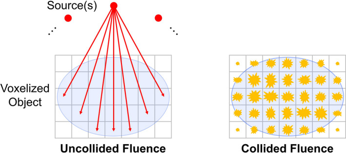
The uncollided fluence at each voxel is determined by ray tracing from the source. If there are multiple sources, it is the sum of all sources. The collided fluence is the solution of the LBTE and represents the secondary (scattered) fluence. [Color figure can be viewed at wileyonlinelibrary.com]
2.B. Phantom study
Our digital phantom study was based on the AAPM Task Group 195 (TG 195): Monte Carlo reference data for imaging research. In particular, Case 5 simulates the dose from a CT scan to a voxelized phantom, which is based on the XCAT phantom.41 The phantom is 320 × 500 × 260 mm3, where each 1 × 1 × 1 mm3 voxel is assigned to one of 20 labels, of which 17 are organs. Each label is assigned a material, whose composition and mass density are defined.
The CT scanner geometry has a 600 mm source–isocenter distance, and the isotropic point source is collimated to a fan beam of width 500 mm and thickness t at isocenter. We reproduced the case of a continuous source distribution along a 360° circular path (axial scan) and the 120 kV spectrum given by TG 195 (Fig. 2).
Figure 2.
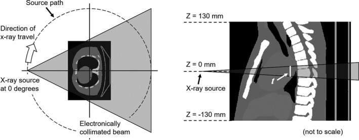
Overview of CT dose simulation with a voxelized phantom, as described in Ref. 36.Not drawn to scale.
The energy deposited per source photon was scored in all voxels and summed for each organ. We used the mean of the four Monte Carlo packages evaluated by TG 195 as the reference value.
2.B.1. Axial fan beam scan
In the TG 195 study, the beam thickness was t = 10 mm and rotated in the Z = 0 mm plane with no table motion, so we refer to this as an axial fan beam scan. By modern standards, this is a relatively thin fan beam. Therefore, we explored two additional geometries, as described next.
2.B.2. Axial cone beam scan
We enlarged the beam to t = 160 mm to model an axial cone beam CT (CBCT) geometry, again with rotation in the Z = 0 mm plane and no table motion. In addition to CBCT systems, such large geometries are increasingly common in diagnostic CT as scanners move toward larger volumetric coverage. All other aspects of the simulation were kept the same.
2.B.3. Helical scan
To model a helical scan, the beam thickness was set to t = 40 mm, and the source was translated from Z = −80 mm to Z = +80 mm, while completing four rotations starting and ending at the zero‐degree position. This simulated a CT acquisition with linear table motion for a helical pitch of 1. All other aspects of the simulation were kept the same.
2.C. Geant4 implementation
We sought to validate our own implementation of Monte Carlo dose calculation against the TG 195 fan beam results. Once validated, our Monte Carlo results could serve as the reference for the cone beam and helical geometries. We used Geant4 (v9.6)37 to randomly sample the spectrum and ray angle for each launched photon and track the energy deposited, using the Livermore physics model, a range cut of 0.1 mm, and the original phantom materials and resolution (1 × 1 × 1 mm3). The fan beam and cone beam simulations used 1 × 10¹⁰ photons and the helical simulation used 4 × 10¹⁰ photons to obtain results with low statistical uncertainty (<1% uncertainty in energy deposited in all organs, and ≪ 1% in organs other than the adrenals and thyroid 36). Geant4 simulations were conducted with an in‐house distributed network of computers (HTCondor, University of Wisconsin, Madison, WI, USA) without any acceleration or variance reduction.
2.D. Acuros implementation
The phantom was cropped laterally by 30 mm on each side to 320 × 440 × 260 mm3 to reduce the volume size, which resulted in a minor amount of truncation in the shoulders. The nonbone materials were decomposed into representative amounts of adipose (ICRP 1975)42 and water that best matched the attenuation properties of the original materials. Bone was added as a third material. Like the original XCAT description, all bone regions are represented by a dense, homogeneous, cortical bone‐like material. This simplified the implementation by reducing the number of unique materials to three. As adipose has a lower effective atomic number (Z eff ) and water has a higher Z eff than most of the nonbone materials, we felt that this approach was supported by the same theory supporting dual‐energy imaging.43, 44
For the fan beam simulation, we used 8 × 8 × 1 mm3 voxels. The 1 mm longitudinal dimension was used to capture the narrow fan beam, while the larger 8 × 8 mm2 in‐plane dimension reduced the number of voxels. The volume was evenly divided by this downsampling factor to 40 × 55 × 260 voxels, and each downsampled voxel was assigned the average material content of its region.
For the cone beam and helical simulations, we used isotropic 5 × 5 × 5 mm3 voxels since the beam was much thicker. This resulted in 64 × 88 × 52 voxels. Unless otherwise stated, we maintained the same voxel size for the uncollided and collided fluences, which allowed the uncollided fluence to seed the first‐scattering source of the collided fluence.
Acuros requires discrete source positions, so we used 18 uniformly spaced source positions per rotation or every 20°. For the helical scan, this resulted in 4 × 18 + 1 = 73 source positions, with the extra one due to having one at the start and stop positions. We also separately studied the impact of the number of source positions and voxel size selection for the cone beam simulation.
Acuros was run on a standard workstation, with the core algorithms written in the CUDA programming language (CUDA 8.0, Nvidia, Santa Clara, CA, USA) and run on a single GPU (GeForce GTX 1080, Nvidia, Santa Clara, CA, USA).
3. Results
3.A. Axial fan beam scan
The spatial distribution of energy deposited for the axial fan‐beam scan is shown in Fig. 3, where the Geant4 and Acuros results are visually identical. In the axial view, the energy distribution is roughly radially symmetric due to the continuous, circular source path, with the exception of the patient posterior shielded by the couch. The narrow fan beam is evident in the coronal and sagittal views, and the secondary dose deposited throughout the volume appears faintly. The difference image shows some disagreement, particularly at the interface between air/tissue and tissue/bone. Acuros tends to underestimate the energy deposited on the entrance side of these interfaces since the calculated fluence is done with relatively large voxels (8 × 8 mm2 in the axial plane) and does not fully resolve the distinct gradient in fluence.
Figure 3.
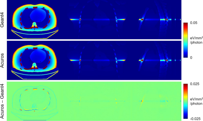
Energy deposited in axial fan beam scan simulation. The top row shows Geant4 results, the middle row shows Acuros, and the bottom row shows the difference. From left to right, the central axial, coronal, and sagittal slices are shown. The jet colormap spans [0 0.05] eV/mm3/photon for the first two rows and [−0.025 0.025] eV/mm3/photon for the last row. [Color figure can be viewed at wileyonlinelibrary.com]
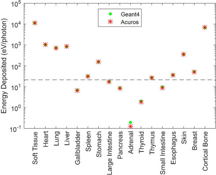
Figure 4 compares the energy deposited in each organ, as reported by TG 195, and as determined from our Geant4 and Acuros simulations. The “soft tissue” and “cortical bone” regions absorb the most energy, in part due to their large size. For bone, this is additionally due to its higher density and higher Z eff . Organs such as the heart, lung, and skin are within the primary beam, while the liver and stomach are not but are large enough to absorb a fair amount of secondary dose. Distant and small organs, such as the adrenals, absorb many orders of magnitude less energy than those in the primary beam. Compared to the TG 195 results, our Geant4 implementation had a max error of 1.4% and root‐mean‐squared error (RMSE) of 0.7% across all organs. Our Acuros solution yielded a max error of 4.8% and RMSE of 2.2% across all organs. However, if we exclude organs that absorb <0.1% of the total energy absorbed, the maximum error decreased to 2.7% and RMSE decreased to 1.4%. The Geant4 results show excellent agreement with TG 195, validating our implementation and enabling us to apply it as the gold standard for other simulations. The good agreement of Acuros across all nonbone organs suggests that the adipose/water material representation was reasonable. Although the Acuros errors were slightly higher than Geant4 due to discretization, the solution was computed in only 15 s. Conversely, the Geant4 results took 687 CPU‐hours to run 1 × 10¹⁰ photons.
Figure 4.
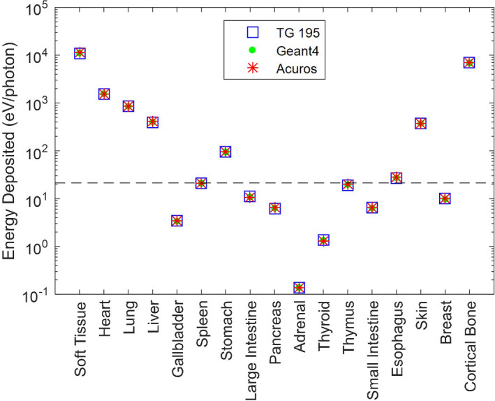
Energy deposited in each organ for the axial fan beam scan simulation. The Geant4 and Acuros results are superimposed on the TG 195 results. Note the log scale of the y‐axis. Organs below the dashed line absorb <0.1% of the total energy absorbed. [Color figure can be viewed at wileyonlinelibrary.com]
3.B. Axial cone beam scan
The Geant4 and Acuros energy deposition maps are shown in Fig. 5 and again exhibit good qualitative agreement. The large cone beam is evident in the coronal and sagittal slices, with secondary dose outside of the beam evident as well. Some stochastic noise can be seen in the Geant4 solution, whereas the Acuros solution does not have any noise. In the sagittal view, there are small visual differences in the spine, which may be due to the challenging combination of thick cortical bone (entire spine is composed of cortical bone, which has higher mass density and Z eff than soft tissue) and discretization effects. The difference image shows good agreement in the soft tissue but some disagreement in the bone, with Acuros slightly overestimating in the ribs and underestimating in the vertebral bodies. The difference at the air/tissue and tissue/bone interfaces is not as distinct as in the fan beam scan, likely due to the smaller voxel size in the axial plane (5 × 5 mm2).
Figure 5.
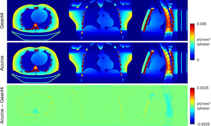
Energy deposited in axial cone beam scan simulation. The jet colormap spans [0 0.005] eV/mm3/photon for the top two rows and [−0.0025 0.0025] eV/mm3/photon for the bottom row. [Color figure can be viewed at wileyonlinelibrary.com]
Nonetheless, using the Geant4 solution as the reference, the Acuros energy deposited per organ (excluding organs with <0.1% of the total energy) had a max error of 2.2% and RMSE of 1.2% (Fig. 6). The adrenals had the largest relative error at 35.9%, likely due to being a small organ far away from the primary beam. However, the error on an absolute scale was 0.066 eV/photon, which is more than five orders of magnitude below the total energy deposited (2.127 × 10⁴ eV/photon). With the isotropic 5 mm voxels, there were fewer voxels overall than the fan beam computation, resulting in a run time of 8 s.
Figure 6.
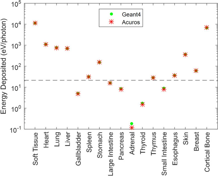
Energy deposited in each organ for the axial cone beam scan simulation. Note the log scale of the y‐axis. Organs below the dashed line absorb <0.1% of the total energy absorbed. [Color figure can be viewed at wileyonlinelibrary.com]
The impact of parameter selection on run time and RMSE is shown in Fig. 7. In Fig. 7(a), the number of uniformly spaced source angles was varied while keeping the voxel size fixed (5 mm isotropic). The run time increased linearly with the number of sources due to the linear increase in ray tracing effort for the uncollided fluence. The RMSE dropped dramatically after five sources and leveled off after around 12 sources. Therefore, 18 sources appeared to be a reasonable selection. In Fig. 7(b), the number of sources was fixed at 18, while voxel size varied. Run time decreased as the voxel size increased (and the number of voxels decreased), while the RMSE increased nearly linearly after 4 mm voxel size. The upper limit on the number of voxels (and the lower limit of voxel size) was constrained by memory requirements, with a 4 mm minimum isotropic voxel size for the collided fluence. Thus, the uncollided fluence for 2 mm isotropic voxels was computed separately. We also kept the longitudinal voxel size to a maximum of 5 mm. Overall, 2–5 mm isotropic voxels appear to be a reasonable selection, depending on the desired run time and accuracy, and subject to memory constraints.
Figure 7.
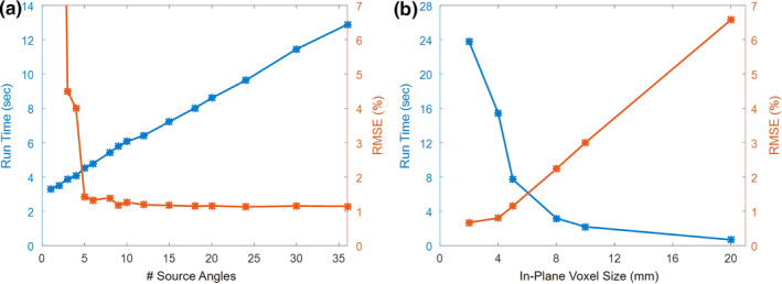
Impact of parameter selection on run time and RMSE. (a) Number of uniformly spaced source angles, using 5 mm isotropic voxels. (b) In‐plane voxel size, using 18 sources. The longitudinal voxel size was kept to a maximum of 5 mm. [Color figure can be viewed at wileyonlinelibrary.com]
3.C. Helical scan
The energy deposited in the phantom by the helical scan is shown in Fig. 8, with excellent agreement between Geant4 and Acuros. The large pitch of the helical pattern and nonuniform dose distribution within the scan range is evident. The difference image shows small disagreement in the soft tissue, for example, some residual helical pattern is evident in the coronal slice due to discretization of the edge of the 40 mm thick beam. The energy deposited in the ribs tends to be overestimated, while it is underestimated in the vertebral bodies. Overall, the quantitative agreement was similar to the cone‐beam scan comparison. Compared to Geant4, Acuros had a max error of 2.3% and RMSE of 1.5%, again excluding organs with <0.1% total energy (Fig. 9). Acuros did take a longer computation time of 23 s due to the increased ray tracing from the 4× increase in the number of sources modeled.
Figure 8.
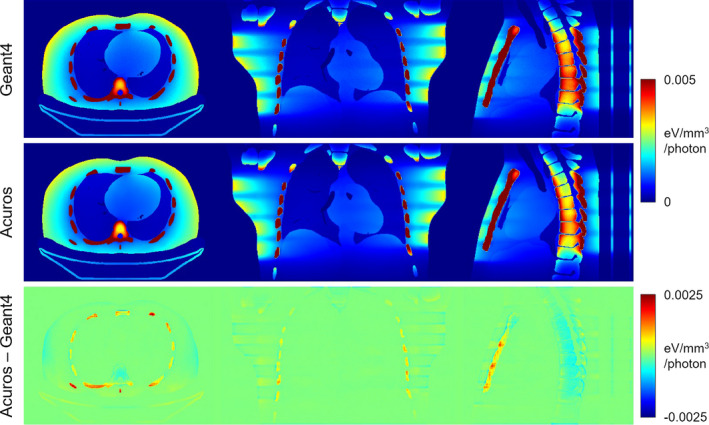
Energy deposited in helical scan simulation. The jet colormap spans [0 0.005] eV/mm3/photon for the top two rows and [−0.0025 0.0025] eV/mm3/photon for the bottom row. [Color figure can be viewed at wileyonlinelibrary.com]
Figure 9.
Energy deposited in each organ for the helical scan simulation. Note the log scale of the y‐axis. Organs below the dashed line absorb <0.1% of the total energy absorbed. [Color figure can be viewed at wileyonlinelibrary.com]
4. Discussion
Using a deterministic solver of the LBTE, such as Acuros, is a new approach to calculating CT dose and potential alternative to Monte Carlo methods. The work in Ref. 29 describes a similar deterministic approach to estimate dose in a uniform CTDI phantom in 21 min. Our work has demonstrated that organ dose calculation in a complex, heterogenous phantom is possible on the order of tens of seconds.
AAPM TG 195 provided a useful benchmark for validating our Geant4 implementation, and although it was designed for Monte Carlo testing, was invaluable for understanding performance of our deterministic method. The fan beam geometry used in TG 195 is a challenging case for Acuros since it required very thin voxels to model the narrow fan beam, leading to a large number of voxels in the longitudinal direction to model the entire volume. The implementation in Acuros CTD uses the same voxel size across the entire volume, but an implementation with adaptive voxel sizes, such as in Acuros XB, could reduce the total number of voxels by using smaller voxels where the fluence is rapidly changing and larger voxels where the fluence is gradually changing.
We observed small voxel‐specific differences near high‐contrast interfaces (i.e., air/tissue or tissue/bone) or within dense, highly attenuating objects (i.e., inside large regions of cortical bone). However, when reporting the total organ energy, some of these differences averaged out, leading to errors less than a few percent. Our analysis mostly excluded small, distant organs (threshold set as <0.1% total energy deposited), where the relative errors tended to be larger even though the absolute errors were small. Should these organs or voxel‐level accuracy be important, the results could be improved by using smaller voxels or finer discretization in other domains. Unlike Monte Carlo, there is no stochastic noise in the solution.
Representation of the phantom materials by a mixture of adipose, water, and bone in our Acuros simulations led to good overall agreement in this study. However, such a representation should be validated against real human tissues or tissue‐equivalent materials in a complex, heterogeneous object. Additionally, patient scans often have contrast media (e.g., iodine, barium) or metal implants, which should be accounted for by using additional materials in Acuros.
We also examined cone beam and helical geometries that are more representative of modern scanners than the TG 195 fan beam geometry. With the larger beams and larger volumetric coverage, we found that 18 source positions per rotation and isotropic 5 mm voxels gave good results for Acuros. The computation time increases with the number of source positions but remains low overall due to the GPU implementation and scales well with the number of sources since the collided fluence is only solved once. Although TG 195 uses an isotropic source collimated to the detector that is uniformly distributed around the object, our Acuros implementation allows each source to be described individually. This enables the modeling of spatial variation (e.g., bowtie or heel effect), variation in intensity between positions (e.g., tube current modulation), and variation in shape between positions (e.g., dynamic collimation). We plan to model these more realistic aspects of scanner behavior and perform validation against physical measurements of a scanned object (e.g., measured dose in a phantom) in future work.
Although we reported run times for our Monte Carlo simulations, these were used to establish reference values with low uncertainty rather than optimized for run time and are not intended for direct comparison with our Acuros run times. Further studies are needed to investigate potential applications of this rapid dose estimation software, as well as to investigate whether there are benefits compared to state‐of‐the‐art Monte Carlo approaches, such as in run time or precision. We plan future work to combine the rapid dose maps generated by Acuros CTD with autosegmentation software to produce automated patient‐specific dose reports.45
5. Conclusion
This study benchmarked the Acuros CTD software for CT organ dose estimation using TG 195. Acuros produced organ dose estimates with maximum error of 2.7% and RMSE below 1.5%, with run time on the order of tens of seconds.
Acknowledgments
This work was supported by NIH U01EB023822. AW, AM, TW, and JSL are or were employees of Varian Medical Systems.
References
- 1. Kase K, No R. 160: Ionizing Radiation Exposure of the Population of the United States. Bethesda, MD: NCRP; 2009. [Google Scholar]
- 2. Brenner DJ, Elliston CD, Hall EJ, Berdon WE. Estimated risks of radiation‐induced fatal cancer from pediatric CT. Am J Roentgenol. 2001;176:289–296. [DOI] [PubMed] [Google Scholar]
- 3. Brenner DJ, Hall EJ. Computed tomography–an increasing source of radiation exposure. N Engl J Med. 2007;357:2277–2284. [DOI] [PubMed] [Google Scholar]
- 4. Einstein AJ, Henzlova MJ, Rajagopalan S. Estimating risk of cancer associated with radiation exposure from 64‐slice computed tomography coronary angiography. JAMA. 2007;298:317. [DOI] [PubMed] [Google Scholar]
- 5. Wintermark M, Lev MH. FDA investigates the safety of brain perfusion CT. Am J Neuroradiol. 2010;31:2–3. [DOI] [PMC free article] [PubMed] [Google Scholar]
- 6. Goske MJ, Applegate KE, Boylan J, et al. Image GentlySM: a national education and communication campaign in radiology using the science of social marketing. J Am Coll Radiol. 2008;5:1200–1205. [DOI] [PubMed] [Google Scholar]
- 7. Sidhu M, Goske M, Coley B, et al. Image gently, step lightly: increasing radiation dose awareness in pediatric interventional radiology. Pediatr Radiol. 2009;39:1135–1138. [DOI] [PubMed] [Google Scholar]
- 8. Morin RL, Coombs LP, Chatfield MB. ACR dose index registry. J Am Coll Radiol. 2011;8:288–29. [DOI] [PubMed] [Google Scholar]
- 9. The Joint Commission . Diagnostic Imaging Requirements. Oakbrook Terrace, IL: The Joint Commission; 2015:1–6. [Google Scholar]
- 10. Bhargavan‐Chatfield M, Morin RL. The ACR computed tomography dose index registry: the 5 million examination update. J Am Coll Radiol. 2013;10:980–983. [DOI] [PubMed] [Google Scholar]
- 11. Brenner DJ, McCollough CH, Orton CG. It is time to retire the computed tomography dose index (CTDI) for CT quality assurance and dose optimization. Med Phys. 2006;33:1189–1191. [DOI] [PubMed] [Google Scholar]
- 12. McCollough CH, Leng S, Yu L, Cody DD, Boone JM, McNitt‐Gray MF. CT dose index and patient dose: they are not the same thing. Radiology. 2011;259:311–316. [DOI] [PMC free article] [PubMed] [Google Scholar]
- 13. Jarry G, DeMarco JJ, Beifuss U, Cagnon CH, McNitt‐Gray MF. A Monte Carlo‐based method to estimate radiation dose from spiral CT: from phantom testing to patient‐specific models. Phys Med Biol. 2003;48:2645–2663. [DOI] [PubMed] [Google Scholar]
- 14. Huda W, Sterzik A, Tipnis S, Schoepf UJ. Organ doses to adult patients for chest CT. Med Phys. 2010;37:842–847. [DOI] [PMC free article] [PubMed] [Google Scholar]
- 15. Choonik L, Choonik L, Robert S, et al. Organ and effective doses in pediatric patients undergoing helical multislice computed tomography examination. Med Phys. 2007;34:1858–1874. [DOI] [PubMed] [Google Scholar]
- 16. Lee C, Kim K, Long D, et al. Organ doses for reference adult male and female undergoing computed tomography estimated by Monte Carlo simulations. Med Phys. 2011;38:1196–1205. [DOI] [PMC free article] [PubMed] [Google Scholar]
- 17. Deak P, van Straten M, Shrimpton PC, Zankl M, Kalender WA. Validation of a Monte Carlo tool for patient‐specific dose simulations in multi‐slice computed tomography. Eur Radiol. 2008;18:759–772. [DOI] [PubMed] [Google Scholar]
- 18. Angel E, et al. Monte Carlo simulations to assess the effects of tube current modulation on breast dose for multidetector CT. Phys Med Biol. 2009;54:497–511. [DOI] [PMC free article] [PubMed] [Google Scholar]
- 19. Zhang D, et al. Reducing radiation dose to selected organs by selecting the tube start angle in MDCT helical scans: a Monte Carlo based study. Med Phys. 2009;36:5654–5664. [DOI] [PMC free article] [PubMed] [Google Scholar]
- 20. Hoppe ME, Schmidt TG. Estimation of organ and effective dose due to Compton backscatter security scans. Med Phys. 2012;39:3396–3403. [DOI] [PubMed] [Google Scholar]
- 21. Gandhi D, Crotty DJ, Stevens GM, Schmidt TG. Technical Note: phantom study to evaluate the dose and image quality effects of a computed tomography organ‐based tube current modulation technique. Med Phys. 2015;42:6572–6578. [DOI] [PubMed] [Google Scholar]
- 22. Jin Y, Yin Z, Yao Y, et al. Patient specific tube current modulation for CT dose reduction. SPIE Med Imaging. 2015;9412:94122Z. [Google Scholar]
- 23. Sperl J, Beque D, Claus B, De Man B, Senzig B, Brokate M. Computer‐Assisted Scan Protocol and Reconstruction (CASPAR)—reduction of image noise and patient dose. IEEE Trans Med Imaging. 2010;29:724–732. [DOI] [PubMed] [Google Scholar]
- 24. Badal A, Badano A. Accelerating Monte Carlo simulations of photon transport in a voxelized geometry using a massively parallel graphics processing unit. Med Phys. 2009;36:4878–4880. [DOI] [PubMed] [Google Scholar]
- 25. Chen W, Kolditz D, Beister M, Bohle R, Kalender WA. Fast on‐site Monte Carlo tool for dose calculations in CT applications. Med Phys. 2012;39:2985–2996. [DOI] [PubMed] [Google Scholar]
- 26. Jia X, Yan H, Gu X, Jiang SB. Fast Monte Carlo simulation for patient‐specific CT/CBCT imaging dose calculation. Phys Med Biol. 2012;57:577–590. [DOI] [PubMed] [Google Scholar]
- 27. George Xu X, Liu T, Su L, et al., ARCHER, a New Monte Carlo Software Tool for Emerging Heterogeneous Computing Environments. in SNA + MC 2013 – Joint International Conference on Supercomputing in Nuclear Applications + Monte Carlo, 2014, p. 06002.
- 28. Mikell J, Cheenu Kappadath S, Wareing T, Erwin WD, Titt U, Mourtada F. Evaluation of a deterministic grid‐based Boltzmann solver (GBBS) for voxel‐level absorbed dose calculations in nuclear medicine. Phys Med Biol. 2016;61:4564–4582. [DOI] [PubMed] [Google Scholar]
- 29. Norris ET, Liu X, Hsieh J. Deterministic absorbed dose estimation in computed tomography using a discrete ordinates method. Med Phys. 2015;42:4080–4087. [DOI] [PubMed] [Google Scholar]
- 30. Vassiliev ON, Wareing T, McGhee J, Failla G, Salehpour MR, Mourtada F. Validation of a new grid‐based Boltzmann equation solver for dose calculation in radiotherapy with photon beams. Phys Med Biol. 2010;55:581–598. [DOI] [PubMed] [Google Scholar]
- 31. Bush K, Gagne IM, Zavgorodni S, Ansbacher W, Beckham W. Dosimetric validation of Acuros XB with Monte Carlo methods for photon dose calculations. Med Phys. 2011;38:2208–2221. [DOI] [PubMed] [Google Scholar]
- 32. Gifford KA, Price MJ, Horton JL, Wareing TA, Mourtada F. Optimization of deterministic transport parameters for the calculation of the dose distribution around a high dose‐rate Ir192 brachytherapy source. Med Phys. 2008;35:2279–2285. [DOI] [PubMed] [Google Scholar]
- 33. Mikell JK, Mourtada F. Dosimetric impact of an I192r brachytherapy source cable length modeled using a grid‐based Boltzmann transport equation solver. Med Phys. 2010;37:4733–4743. [DOI] [PubMed] [Google Scholar]
- 34. Maslowski A, Wang A, Sun M, Wareing T, Davis I, Star‐Lack J. Acuros CTS: a fast, linear Boltzmann transport equation solver for computed tomography scatter – Part I: core algorithms and validation. Med Phys. 2018;45:1899–1913. [DOI] [PMC free article] [PubMed] [Google Scholar]
- 35. Wang A, Maslowski A, Messmer P, et al. Acuros CTS: a fast, linear Boltzmann transport equation solver for computed tomography scatter – Part II: system modeling, scatter correction, and optimization. Med Phys. 2018;45:1914–1925. [DOI] [PubMed] [Google Scholar]
- 36. Sechopoulos I, et al. Monte Carlo reference data sets for imaging research: executive summary of the report of AAPM Research Committee Task Group 195. Med Phys. 2015;42:5679–5691. [DOI] [PubMed] [Google Scholar]
- 37. Agostinelli S, Allison J, Amako KA, et al. Geant4—a simulation toolkit. Nucl Instrum Methods Phys Res A. 2003;506:250–303. [Google Scholar]
- 38. Lewis EE, Miller WF. Computational Methods of Neutron Transport. New York, NY: John Wiley and Sons Inc; 1984. [Google Scholar]
- 39. Vassiliev ON. Grid based Boltzmann equation solvers. In Monte Carlo Methods for Radiation Transport. Cham, Switzerland: Springer; 2017:225–250. [Google Scholar]
- 40. Hubbell JH, Seltzer SM. Tables of X‐Ray Mass Attenuation Coefficients and Mass Energy‐Absorption Coefficients 1 keV to 20 MeV for Elements Z = 1 to 92 and 48 Additional Substances of Dosimetric Interest. Gaithersburg, MD: NIST; 1995. [Google Scholar]
- 41. Segars WP, Mahesh M, Beck TJ, Frey EC, Tsui BMW. Realistic CT simulation using the 4D XCAT phantom. Med Phys. 2008;35:3800–3808. [DOI] [PMC free article] [PubMed] [Google Scholar]
- 42. Snyder W, Cook M, Nasset E, Karhausen L, Parry Howells G, Tipton I. ICRP Publication 23: Report of the Task Group on Reference Man. Elmsford, NY: The International Commission on Radiological Protection, 1975. [Google Scholar]
- 43. Alvarez RE, Macovski A. Energy‐selective reconstructions in X‐ray computerized tomography. Phys Med Biol. 1976;21:733–744. [DOI] [PubMed] [Google Scholar]
- 44. Brody WR, et al. Dual‐energy projection radiography: initial clinical experience. Am J Roentgenol. 1981;137:201. [DOI] [PubMed] [Google Scholar]
- 45. Schmidt TG, Wang AS, Coradi T, Haas B, Star‐Lack JM. Accuracy of patient‐specific organ dose estimates obtained using an automated image segmentation algorithm. J Med Imaging. 2016;3:43502. [DOI] [PMC free article] [PubMed] [Google Scholar]