Singular Value Decomposition Method To Determine Distance Distributions in Pulsed Dipolar Electron Spin Resonance: II. Estimating Uncertainty

Abstract

This paper is a continuation of the method introduced by Srivastava and Freed (2017) that is a new method based on truncated singular value decomposition (TSVD) for obtaining physical results from experimental signals without any need for Tikhonov regularization or other similar methods that require a regularization parameter. We show here how to estimate the uncertainty in the SVD-generated solutions. The uncertainty in the solution may be obtained by finding the minimum and maximum values over which the solution remains converged. These are obtained from the optimum range of singular value contributions, where the width of this region depends on the solution point location (e.g., distance) and the signal-to-noise ratio (SNR) of the signal. The uncertainty levels typically found are very small with substantial SNR of the (denoised) signal, emphasizing the reliability of the method. With poorer SNR, the method is still satisfactory but with greater uncertainty, as expected. Pulsed dipolar electron spin resonance spectroscopy experiments are used as an example, but this TSVD approach is general and thus applicable to any similar experimental method wherein singular matrix inversion is needed to obtain the physically relevant result. We show that the Srivastava—Freed TSVD method along with the estimate of uncertainty can be effectively applied to pulsed dipolar electron spin resonance signals with SNR > 30, and even for a weak signal (e.g., SNR ≈ 3) reliable results are obtained by this method, provided the signal is first denoised using wavelet transforms (WavPDS).

Graphical Abstract

1. INTRODUCTION

1.A. Background.

In many physical systems, methods based on singular value decomposition (SVD) are used to process data to elicit desired results.^1–8 However, uncertainty determination in the resultant outcome has remained a challenge and is needed to reliably interpret the results. There have been some efforts to determine uncertainty such as for pulsed dipolar electron spin resonance (ESR) experiments using Tikhonov regularization or model fitting, but they focused on the overall outcome^9,10 of the effects of noise present in experimental signals and on other factors such as the background signal.¹⁰ However, the uncertainty generated due to the SVD process has received little attention but is considered here in the context of the SVD method introduced by Srivastava and Freed (SF),⁷ which is a new and improved method based on the truncated SVD (TSVD).¹¹ The SF method leads to accurate solutions for singular matrix inversion by introducing a rigorous cutoff that is a function of the output location. Herein, we show how to determine the uncertainty in this SF-TSVD method both for high and low SNR. This requires one to determine uncertainty at each output location instead of calculating an overall uncertainty, which is not appropriate. We illustrate this approach by successfully applying it to experimental pulsed dipolar ESR signals. Improvements in ESR instrument technology^2,12–15 and developments in data-processing methods, such as wavelet denoising,^16,17 have enabled us to obtain ESR signals with very high signal-to-noise ratio (SNR) as well as with excellent fidelity.

We describe this method to quantify the uncertainty resulting from the SVD-based reconstruction of physical experiments such as ESR, wherein singular matrix inversion is required to obtain the physically relevant result, especially in the presence of finite noise. Our previous work has shown that the SVD solution at each output point (e.g., value of r) can be optimized but after a different number of singular value contributions (SVCs) before becoming unstable.⁷ We show in this paper using the ESR data that this uncertainty in optimization at each output point is not uniform and varies among such points. Thus we determine the uncertainty at each location of the output independently based on the SVCs. (In our previous paper,⁷ we used the term “convergence”, but “optimization” is a better word because in many cases there is no simple convergence to a constant or asymptotic value but rather to an “optimum region”.)

1.B. Pulsed Dipolar Spectroscopy.

We demonstrate the method using pulsed dipolar ESR spectroscopy (PDS) as an example as in our previous study. PDS plays a key role in determining the structure and dynamics of biological systems.^2,18–25 In PDS, paramagnetic tags^26,27 called spin labels (NO, Cu²⁺, among others) are attached at specific locations; then, a dipolar signal is acquired from the interaction between a pair of spin labels, from which the distance distribution between them, P(r), may be obtained. A Fredholm equation of the first kind can be used to represent the system in the following way

$$S(t)={\int }_{R_{\text{min}}}^{R_{\text{max}}}\kappa (r,t)P(r)\mathrm{d}r$$ (1)

The dipolar signal S(t) is acquired from the experiment, whereas the kernel κ(r,t) contains the dipolar interaction between spin pairs and is generated from theory as a function of time t and distance r. The distance distribution P(r) is constructed using a mathematical inversion process involving the dipolar signal S and a kernel matrix K. The mathematical representation in matrix notation is as follows

$$\mathit{KP}=S$$ (2)

The matrix dimensions of K, P, and S are M × N, N × 1, and M × 1, respectively, where N ≤ M. One wishes to obtain the distance distribution P given K and S. Because K is a singular matrix, mathematical inversion (P = K⁻¹S) cannot be obtained simply.

2. PREVIOUS METHODS

2.A. Tikhonov Regularization, Its SVD Form, and Its Uncertainty with Respect to Regularization Parameter (λ).

Tikhonov regularization (TIKR) has been traditionally used to obtain the distance distribution P when noise is present in the signal. It minimizes the following function^8,28

$${\varphi }_{\text{TIKR}}\left[P\right]\equiv \text{min}({\Vert \mathit{KP}-S\Vert }^2+{\mathit{\lambda }}^2{\Vert \mathit{LP}\Vert }^2)$$ (3)

where λ is the regularization parameter and L is a differential operator. The solution P_λ can be obtained as

$$P_{\mathit{\lambda }}={(K^{T}K+{\mathit{\lambda }}^2)}^{-1}{K}^{T}S$$ (4)

Equation 4 can be reduced to SVD form in the following way

$$P_{\mathit{\lambda }}={({\Sigma }^2+{\mathit{\lambda }}^{2}I)}^{-1}V\Sigma U^{T}S$$ (5)

where the K matrix is decomposed in the SVD form as

$$K=U\Sigma V^T$$ (6)

where U and V are orthogonal matrices with dimensions M × M and N × N, respectively, and ∑ is an M × N diagonal matrix consisting of non-negative singular values in decreasing order.

Using eq 5, the solution P_λ can be rewritten as a modified sum i over SVCs as

$$P_{\mathit{\lambda }}=\sum _{j=1}^N\sum _{i=1}^{{\sigma }_i>\mathit{\lambda }}\sum _{l=1}^M{f}_i{V}_{\mathit{ji}}{\left({\Sigma }^{-1}\right)}_{\mathit{ii}}{U_{\mathit{il}}}^T{S}_l$$ (7)

where j, i, and l are row and column indices. For physical interpretation, j is the index that represents the discretized distance, l represents the discretized time, and i is the index representing the particular singular value. The diagonal matrix ∑⁻¹ contains the reciprocal of the singular values, that is, the $\left(\frac{1}{{\sigma }_i}\right)$, and f_i is a filter function,²⁸ defined as $f_i\equiv \frac{{\sigma }_i^2}{{\sigma }_i^2+{\mathit{\lambda }}^2}$, that suppresses the SVCs from small singular values for which ${\sigma }_i^2\ll {\mathit{\lambda }}^2$. The choice of λ is crucial; a common approach is to obtain it by the L-curve method,^29,30 but other methods such as generalized cross validation and the Akaike information criterion to select the regularization parameter can also be used.³¹

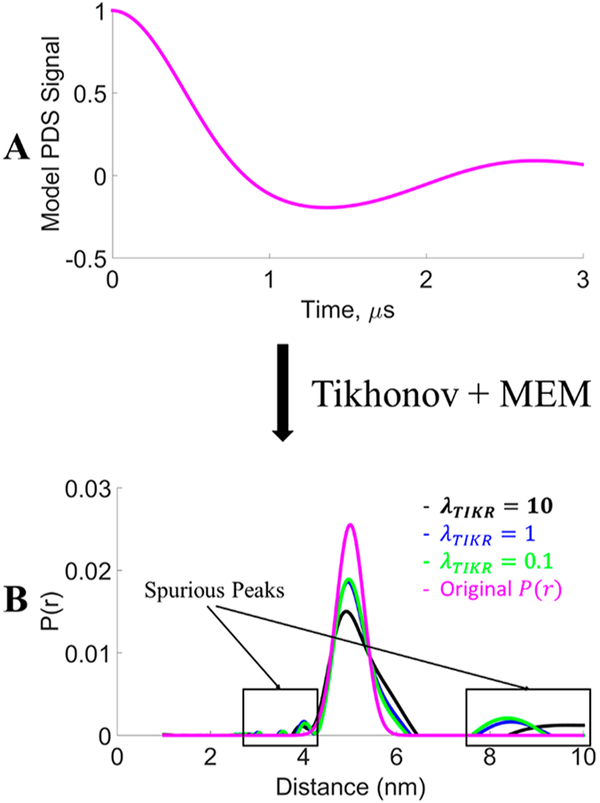
Tikhonov regularization is applied to yield a P(r) that is a compromise between good resolution and stability of the solution. It is dependent on the choice of λ to yield a satisfactory P(r). More importantly, the uncertainty in distance distribution caused by selection of the λ value is not known. In Figure 1, it is shown that selection of different λ values results in different degrees of resolution in P(r), which now contain spurious peaks, even for this noise-free model dipolar signal with a simple unimodal distribution. As can be seen, there is considerable uncertainty in the width of the distribution with different selection of λ values. The optimal choice of λ becomes more challenging when finite noise is present.

Figure 1.

Comparison of distance distributions of a model signal (A) using Tikhonov regularization with different λ values. The model P(r) is a Gaussian distribution centered at 5 nm with standard deviation of 0.3 nm (B). The maximum entropy method (MEM)²⁸ was used to constrain P(r) ≥ 0, suppressing the regions of P(r) < 0 in the original Tikhonov result. Reprinted with permission from ref 17. Copyright 2017 ACS.

2.B. Theorem for Obtaining Exact Solution Using SVD.

For a system of linear equations KP = S, where K is an M × N matrix (N ≤ M) with a rank k (k < M), P is a vector with length N, and S is a vector with length M, there exists an exact solution using SVD if and only if S is orthogonal to the M–k left-singular vectors of K.³² To illustrate, in SVD form, KP = S using eq 6 can be written as

$$U\Sigma V^{T}P=S$$ (8)

To solve for P, eq 8 can be rewritten as

$$P=V{\Sigma }^{-1}{U}^{T}S$$ (9)

or

$$P=\sum _{j=1}^N\sum _{i=1}^N\sum _{l=1}^M{V}_{\mathit{ji}}{\left({\Sigma }^{-1}\right)}_{\mathit{ii}}{U_{\mathit{il}}}^T{S}_l$$ (10)

Which can be written as

$$P=\sum _{j=1}^N\sum _{i=1}^k\sum _{l=1}^M{V}_{\mathit{ji}}{\left({\Sigma }^{-1}\right)}_{\mathit{ii}}{U_{\mathit{il}}}^T{S}_l+\sum _{j=1}^N\sum _{i=k+1}^N\sum _{l=1}^M{V}_{\mathit{ji}}{\left({\Sigma }^{-1}\right)}_{\mathit{ii}}{U_{\mathit{il}}}^T{S}_l$$ (11)

where those for k < i ≤ N are the zeros.

The theorem states³² that if ${\sum }_{l=1}^M{U_{\mathit{il}}}^T{S}_l=0$, ∀ i ∈ [k + 1, M], then the linear system has an exact solution for P and can be obtained as

$$P=\sum _{j=1}^N\sum _{i=1}^k\sum _{l=1}^M{V}_{\mathit{ji}}{\left({\Sigma }^{-1}\right)}_{\mathit{ii}}{U_{\mathit{il}}}^T{S}_l$$ (12)

A more detailed description is given in ref 32. One can compare this to eq 7, wherein f_i may now be considered as equal to unity for i ≤ k and equal to zero for i > k. Equation 12 represents the truncated SVD in which a single singular value cutoff is used to obtain P(r). The truncated SVD approach is well suited when the kernel matrix K has a well-determined numerical rank,¹¹ and the singular value cutoff k can be selected such that it is equal to the rank of the kernel matrix, as demonstrated by Hansen.¹¹ For ill-determined numerical rank of K, one can obtain a desirable P(r) if the Picard condition^8,33 is satisfied¹¹ such that ${U_{\mathit{il}}}^T{S}_l$ decays sufficiently faster than (∑⁻¹)_ii and has a clear divergence point. The Picard condition is given as

$$[\text{Picard}]\equiv \sum _{i=1}^q{\left(\sum _{l=1}^M{\left({\Sigma }^{-1}\right)}_{\mathit{ii}}{U_{\mathit{il}}}^T{S}_l\right)}^2<\infty$$ (13)

for which adding the q + 1 contribution to eq 13 leads to a divergence

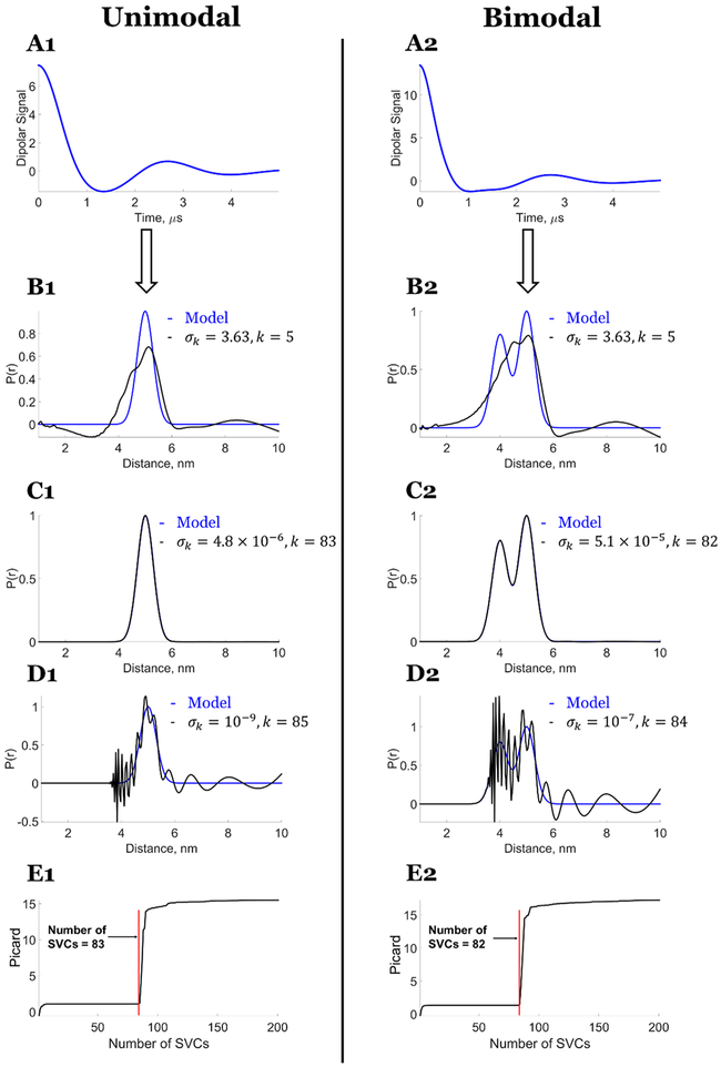
Figure 2 shows that the exact solution for unimodal and bimodal P(r) can be obtained (cf. Figure 2C1,C2) for the noise-free model dipolar signal, for which the condition ${\sum }_{l=1}^M{U_{\mathit{il}}}^T{S}_l=0$, ∀ i ∈ [k + 1, M] is satisfied (cf. Figure 3), which also implies that the kernel K has a well-determined rank. An exact singular value cutoff can be conveniently determined by using the Picard condition that informs about the precise location of divergence of the solution.

Figure 2.

Model data: Exact solution using the SVD method: P(r) versus number of singular value contributions (SVCs). Unimodal distance distribution: (A1) Noise-free dipolar signal. Comparison of model distribution with P(r) generated from (B1) fewer SVCs k = 3, σ_k = 8.04, (C1) exact solution obtained for k = 83, σ_k = 4.8 × 10⁻⁶, (D1) more SVCs k = 85, σ_k = 10⁻⁹, and (E1) Picard plot of ${\log }_{10}\left({\sum }_i{\mid {\sum }_{l=1}^M{\left({\Sigma }^{-1}\right)}_{\mathit{ii}}{U_{\mathit{il}}}^T{S}_l\mid }^2\right)$ versus the number of singular values from k = 1 to 200 starting from largest value. It shows the contributions of singular values that lead to stable and unstable distributions. Bimodal distance distribution: (A2) Noise-free dipolar signal. Comparison of model distribution with P(r) generated from (B2) fewer SVCs k = 3, σ_k = 8.04, (C2) exact solution obtained for k = 82, σ_k = 5.1 × 10, (D2) more SVCs k = 84, σ_k = 10⁻⁷, and (E2) Picard plot of ${\log }_{10}\left({\sum }_i{\mid {\sum }_{l=1}^M{\left({\Sigma }^{-1}\right)}_{\mathit{ii}}{U_{\mathit{il}}}^T{S}_l\mid }^2\right)$ versus the number of singular values from k = 1 to 200 starting from largest value. It shows the contributions of singular values that lead to stable and unstable distributions.⁷ Reprinted with permission from ref 7.

Figure 3.

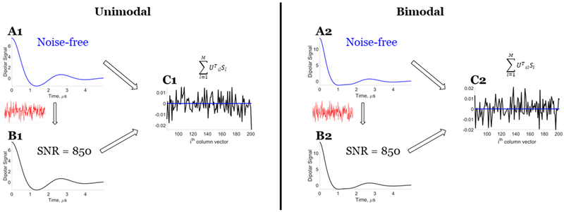
Model data: Orthogonality validation for the noiseless data and data with some noise (SNR ≈ 850). Unimodal distance distribution: (Al) noiseless data, (B1) data with some noise, and (C1) comparison of results of ${\sum }_{l=1}^M{U_{\mathit{il}}}^T{S}_l$ at the ith column vector for noiseless data and data with some noise. Bimodal distance distribution: (A2) noiseless data, (B2) data with some noise, and (C2) comparison of results of ${\sum }_{l=1}^M{U_{\mathit{il}}}^T{S}_l$ at the ith column vector for noiseless data and data with some noise. Signal in red is noise added to the noise-free data (blue) to obtain data with some noise (black). The orthogonality requirement shown in panel C is clearly met for the noiseless data but not for data with some noise. Reprinted with permission from ref 7.

The Picard plots provide the singular value cutoff points (q of 83 and 82, respectively, for the unimodal and bimodal distribution in agreement with the results in Figure 2C1,C2) after which the solution P(r) diverges, which can be seen in Figure 2E1,E2 (red line). That is, the cutoff values of q in eq 13 exactly reproduce the correct k values for eq 12. So we will replace q by k in the following. The Picard plots are best obtained using the formula ${\log }_{10}\left({\sum }_i{\mid {\left({\Sigma }^{-1}\right)}_{\mathit{ii}}{U_{\mathit{il}}}^T{S}_l\mid }^2\right)$, which is the log of eq 13 to reduce the divergence that occurs.

Figure 2 also shows that premature (cf. Figure 2B1,B2) and delayed selection (cf. Figure 2D1,D2) of a singular value cutoff leads to undesirable results. The singular value cutoff at σ_k = 3.63 yields a poorly resolved P(r), whereas the singular cutoff at and above σ_k = 10⁻⁷ yields an unstable solution.

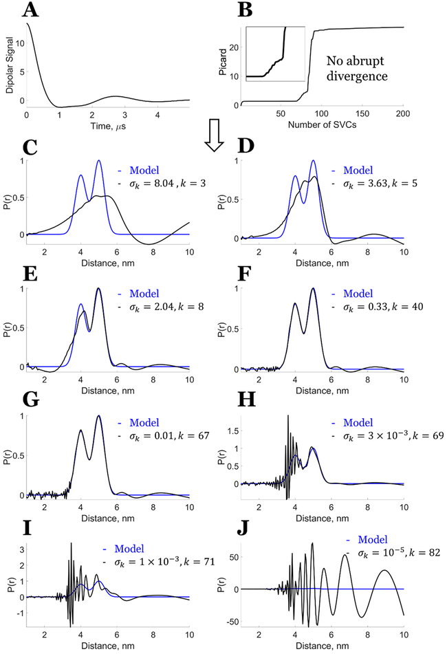
However, in the presence of noise in the signal, the theorem is, in general, not applicable because the condition ${\sum }_{l=1}^M{U_{\mathit{il}}}^T{S}_l=0$, ∀ i ∈ [k + 1, M] is not satisfied (cf. Figure 3). Hence, the single singular value cutoff (or truncated SVD) will not yield the exact solution but will yield a solution in a least-squares sense,³² although it is still favorable compared with the Tikhonov regularization because it will be less sensitive to noise than the Tikhonov regularization.¹¹ Figure 4 and Figure S1 show that there is no longer a clear singular value cutoff k for the distance distribution at which one can get the desired solution, even at an SNR ≈ 850. The Picard plots (Figure 4B and Figure S1B) reflect this, as there is not an abrupt divergence for the solution. They also show that the optimal choice for k is ca. 40–67 for Figure 4 and ca. 40–69 for Figure S1, but this range shows both positive and negative distortions in P(r).

Figure 4.

Model data with some noise (SNR ≈ 850): Bimodal distance distribution. (A) Noisy model data dipolar signal. (B) Picard plot of the bimodal distribution from the noisy model data at different number of singular value contributions (SVCs) represented by i, the enlarged inset covers SVCs from 55 to 90. (C–J) Comparison of model distribution with the distance distribution generated from (C) k = 3, σ_k = 8.04, (D) k = 5, σ_k = 3.63, (E) k = 8, σ_k = 2.04, (F) k = 40, σ_k = 0.33, (G) k = 67, σ_k = 0.01, (H) k = 69, σ_k = 3 × 10⁻³, (I) k = 71, σ_k = 1 × 10⁻³, and (J) k = 82, σ_k = 10⁻⁵. Reprinted with permission from ref 7.

2.C. Distance Distribution Reconstruction in PDS Using New SVD Approach.⁷

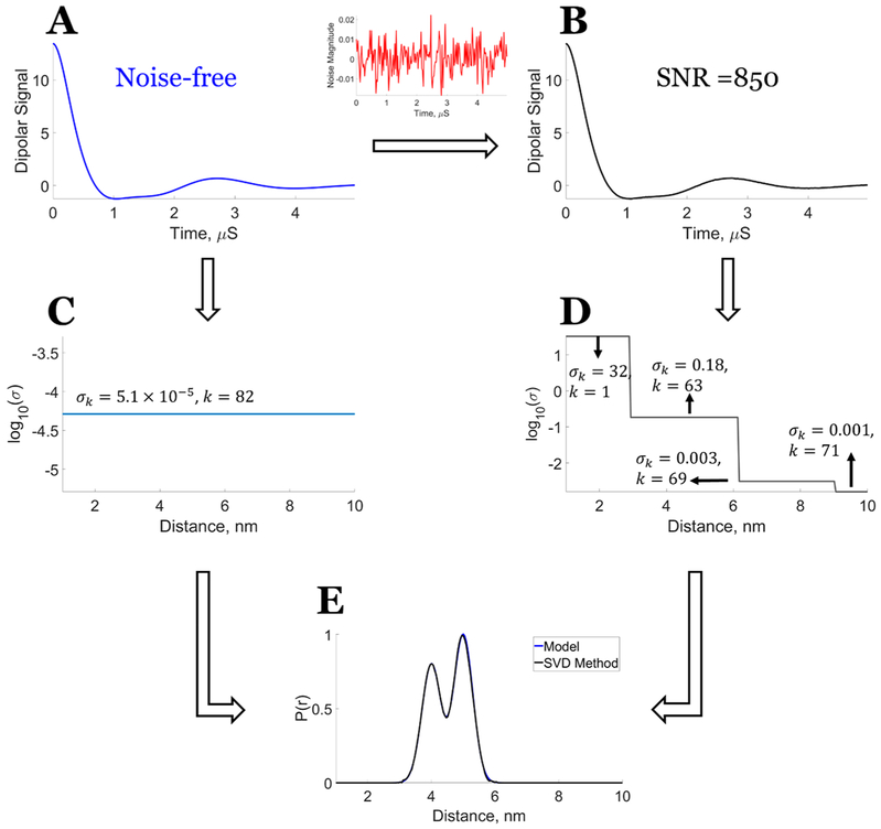
It was shown in our previous paper⁷ that the imperfections of the SVD solution in the presence of noise can be remedied by requiring individual singular value cutoffs for each distance or distance range, as shown in Figure 5 and Figure S2 (for bimodal and unimodal cases, respectively). One sees in these Figures that the correct solution to P(r) is obtained without any of the spurious peaks and negative excursions exhibited in Figure 4 and Figure S1, where a single cutoff k independent of r was used.

Figure 5.

Bimodal model: Reconstruction of distance distribution for noise-free model data and noisy model data (SNR ≈ 850) using the new SVD method. (A) Model dipolar signal. (B) Model dipolar signal with added noise (see added noise in red plot). (C) Singular value cutoff at each distance (nm) for the model dipolar signal. (D) Singular value cutoff at each distance range (nm) for the model dipolar signal with added noise. (E) Distance distribution reconstructed from the model dipolar signal and model dipolar signal with noise using the singular value cutoffs shown in panels C and D, respectively. Note that the added noise is so small that panels A and B still appear identical, but convergence to the virtually identical final results requires the segmentation shown in panel D in the latter case. Reprinted with permission from ref 7.

For this method,⁷ we rewrite eq 12 as

$$P_j=\sum _{i=1}^{k_j}\sum _{l=1}^M{V}_{\mathit{ji}}{\left({\Sigma }^{-1}\right)}_{\mathit{ii}}{U_{\mathit{il}}}^T{S}_l\equiv \sum _{i=1}^{k_j}{\left({\mathit{SVC}}_j\right)}_i$$ (14)

where k_j is the number of nonzero singular values associated with jth index of distance. We refer to each term in the sum over i of eq 14 given by $\left({\left({\Sigma }^{-1}\right)}_{\mathit{ii}}{V}_{\mathit{ji}}{\sum }_{i=1}^M{U_{\mathit{il}}}^T{S}_l\right)$ as the singular value contribution (SVC_j)_i to P_j associated with singular value σ_i.

The solution of P_j should be obtained for each distance value j, as given in eq 14. This is because for signals with noise each P_j is, in general, optimized at a different singular value cutoff k_j before becoming unstable. One can select a single singular value cutoff kj, but there still could be a range of optimum cutoffs before the result becomes unstable, as we discuss below. (Note that the sum over i is taken over decreasing singular values, σ_i).

The use of f_i in Tikhonov regularization provides a “softer” suppression than the sharp suppression in the new SVD method, where the i = k_jth SVC is kept and all SVC’s for i > k_j are set to zero. Tikhonov regularization has not been implemented with r dependence; it solves a least-squares problem using a single λ.

3. UNCERTAINTY DETERMINATION

The uncertainty estimate using the SF-TSVD method is determined by identifying the optimum region, which exists from just after convergence to just before divergence of P(r_j) with respect to SVCs. Prior to convergence, solution P(r_j) is not stable, and after divergence, the solution P(r_j) is certainly not, as can be seen from the Picard plots as well as the P(r_j) values themselves. The variation in p(r_j) in the optimum region is taken as the uncertainty in the solution.

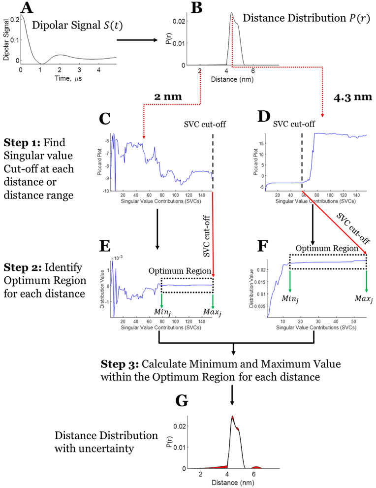
This uncertainty of the distribution for each distance (or distance range) is determined using the following three steps. The example used to demonstrate these steps is an experimental unimodal distribution obtained from a T4 Lysozyme sample (cf. Section 4.A, case 1, for more details)

3.A. Determination of Singular Value Cutoff.⁷

The singular value cutoff is determined for each distance labeled by the index j after which the distribution value becomes unstable. This is accomplished using a modified Picard condition, in which eq 13 is now written as

$${\left[\text{Picard}\right]}_j={\log }_{10}\left({\left(\sum _{i=1}^{k_j}\sum _{l=1}^M{V}_{\mathit{ji}}{\left({\Sigma }^{-1}\right)}_{\mathit{ii}}{U_{\mathit{il}}}^T{S}_l\right)}^2\right)<\infty$$ (15)

where 1 ≤ k_j < M. (Note that eq 15 is the form used in ref 7, but this equation does not explicitly appear there.) Compared with eq 13, this modified Picard condition informs about the convergence of the solution for each j by incorporating V_ji. Furthermore, the square after the summation better dramatizes the point of divergence. In eq 15, the numerator (V_jiU_il^TS_l) should decay sufficiently faster than the denominator $({\Sigma }_{\mathit{ii}}^{-1}={}^1∕_{{\sigma }_i})$ for the solution to remain converged. The k_j is taken as the last singular value σ_kj, after which the solution diverges for that j. Figure 6C,D shows modified Picard plots at 2 and 4.3 nm for the unimodal distribution (Figure 6B).

Figure 6.

Stepwise process of obtaining uncertainty in the distance distribution from the dipolar signal. (A) Denoised experimental dipolar signal using WavPDS (cf. Figure 7 for noisy data). (B) Distance distribution reconstructed using the SVD method.⁷ (C) Modified Picard plot for the 2 nm distance, revealing that the solution for this distance never diverges. Hence, the last data point is selected as SVC cutoff. (D) Modified Picard plot for the 4.3 nm distance, revealing the singular value cutoff before which solution at this distance diverges. (E) P(r) values obtained at the 2 nm distance by different SVCs until the SVC cutoff; if it never diverges as in this case then the last SVC is selected as cutoff. (F) P(r) values obtained at the 4.3 nm distance by different SVCs until the SVC cutoff. (G) Distance distribution with uncertainty in distribution shown in red.

3.B. Identification of Minimum and Maximum SVCs in the Optimum Range.

The SVCs in the sum over i in eq 14, at which the distribution is converged and remains so, need to be determined. The maximum value of i in the converged region or Max_j can be found with the help of the modified Picard plot to determine the k_j given that the following SVCs diverge. The selection of the minimum Min_j is aided by plotting the P(r) values as a function of the added SVCs. It is at the onset of the region where the solution remains stable (or converged), (i.e., flat and nearly constant, which we refer to as the optimum region). Min_j is may be identified visually from the plot of P(r), cf. Figure 6E,F. That is, it is the starting singular value where this “flat” region begins. An objective approach for locating Min_j is to measure the cumulative difference between the minimum and maximum values of P_j as a function of SVCs removed, starting from the Max_j value and moving in the direction of decreasing numbers of SVCs in the optimum region. The difference between the minimum and maximum value in the optimum region will stabilize, but just after Min_j is reached this difference starts to increase significantly with every additional SVC removed (e.g., 50%). A series of five consecutive significant changes each by at least 50% allows the identification of Min_j, which will be the SVC value just before these consecutive changes occur. Figure 6E,F show the values at 2 and 4.3 nm for the unimodal distribution, revealing the converged ranges, which are contained in the rectangular boxes corresponding to the “optimum regions”. We discuss this further in Section 4.B.

3.C. Minimum and Maximum Value of the Distance in the Min–Max SVC Range.

One examines the values of P_j within the optimum range, that is, those with index i lying between Min_j and Max_j, and selects the minimum P_j value $\left(P_j^{\text{Min}}\right)$ and the maximum P_j value $\left(P_j^{\text{Max}}\right)$ within this optimum region. The uncertainty ranges within the $P_j^{\text{Min}}$ and $P_j^{\text{Max}}$ values.

4. RESULTS AND DISCUSSION

4.A. Experimental Data.

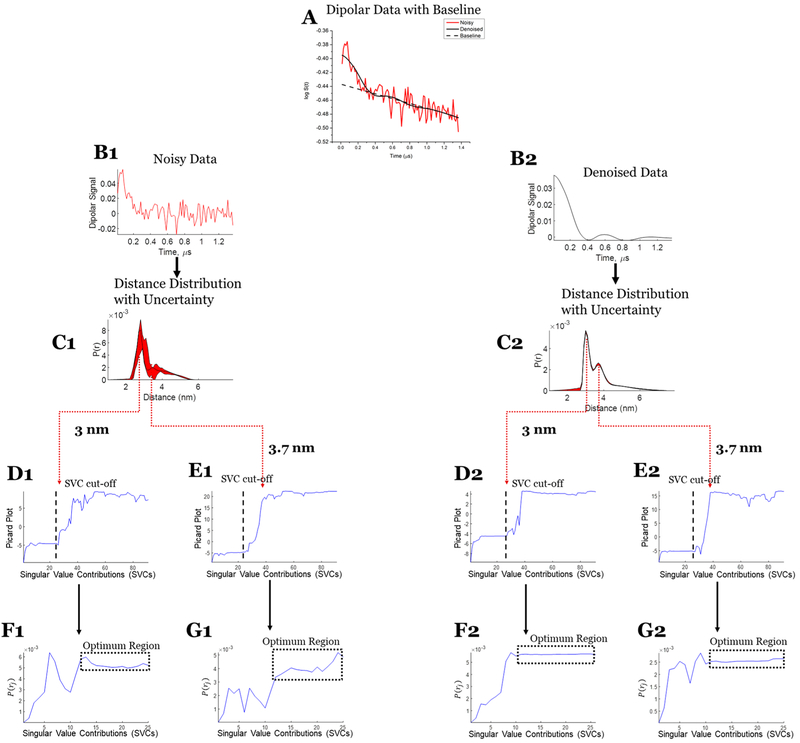
Three sets of experimental data are used to illustrate the uncertainty analysis. Case 1 (cf. Figure 7) consists of a unimodal distribution from T4 lysozyme (T4L), where the 63 μM protein sample is of spin-labeled T4L mutant 44C/135C. The signal was averaged for 952 min to obtain an SNR of 37. In case 2 (cf. Figure 8), a bimodal distribution was used that is also generated from T4L, where the sample is a mixture of mutants spin-labeled at 8C/44C and 44C/135C with concentrations of 44 and 47 μM, respectively. The dipolar signal was acquired after signal averaging for 360 min to obtain an SNR of 80. The data from the samples are the same as those used in both the WavPDS method paper¹⁷ and the SVD paper.⁷ Case 3 (cf. Figure 9) is also from a sample with a bimodal distribution but at a submicromolar concentration. The sample is a spin-labeled Immunoglobulin E (IgE) cross-linked with trivalent DNA–DNP ligand in phosphate-buffered saline (PBS) buffer.^7,34 The dipolar signal was obtained after 18 h of signal averaging, resulting in an SNR of only 3.8. The WavPDS method was then applied to remove the noise from the dipolar signals in all three cases (cf. Figures 7A2, 8A2, and 9B2).

Figure 7.

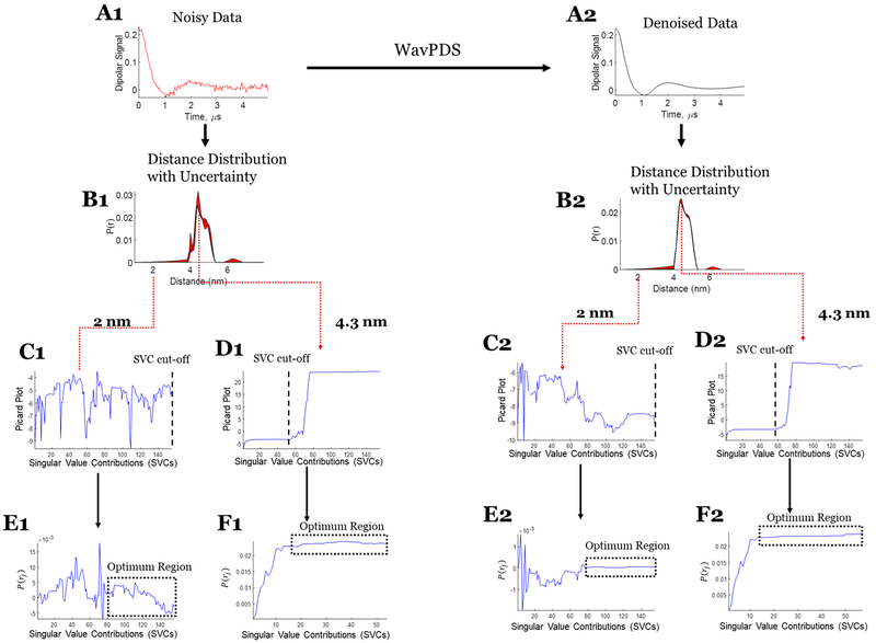
Case 1: SVD reconstruction with uncertainty analysis of the noisy and denoised dipolar signal for unimodal distribution. (A1) Noisy data. (B1) Distance distribution from noisy data with uncertainty (in red). (C1) Modified Picard plot for the 2 nm distance, revealing that the solution for this distance never diverges. Hence, the last data point is selected as SVC cutoff. (D1) Modified Picard plot for the 4.3 nm distance, revealing the singular value cutoff before which solution at this distance diverges. (E1) P(r) values obtained at the 2 nm distance by different SVCs until the SVC cutoff; if it never diverges, as in this case, then the last SVC is selected as cutoff. (F1) P(r) values obtained at the 4.3 nm distance by different SVCs until the SVC cutoff. (A2) Denoised data using WavPDS. (B2) Distance distribution from denoised data with uncertainty (in red). (C2) Modified Picard plot for the 2 nm distance, revealing that the solution for this distance never diverges. Hence, the last data point is selected as SVC cutoff. (D2) Modified Picard plot for the 4.3 nm distance, revealing the singular value cutoff before which solution at this distance diverges. (E2) P(r) values obtained at the 2 nm distance by different SVCs until the SVC cutoff; if it never diverges, as in this case, then the last SVC is selected as cutoff. (F2) P(r) values obtained at the 4.3 nm distance by different SVCs until the SVC cutoff.

Figure 8.

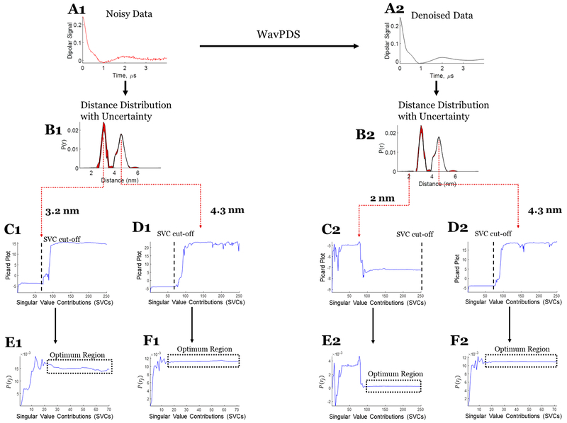
Case 2: SVD reconstruction with uncertainty analysis of the noisy and denoised dipolar signal for bimodal distribution. (A1) Noisy data. (B1) Distance distribution from noisy data with uncertainty (in red). (C1) Modified Picard plot for the 3.2 nm distance, revealing the singular value cutoff before which solution at this distance diverges. (D1) Modified Picard plot for the 4.3 nm distance, revealing the singular value cutoff before which solution at this distance diverges. (E1) P(r) values obtained at the 3.2 nm distance by different SVCs until the SVC cutoff; if it never diverges, as in this case, then the last SVC is selected as cutoff. (F1) P(r) values obtained at the 4.3 nm distance by different SVCs until the SVC cutoff. (A2) Denoised data using WavPDS. (B2) Distance distribution from denoised data with uncertainty (in red). (C2) Modified Picard plot for the 2 nm distance, revealing that the solution for this distance never diverges. Hence, the last data point is selected as SVC cutoff. (D2) Modified Picard plot for the 4.3 nm distance, revealing the singular value cutoff before which solution at this distance diverges. (E2) P(r) values obtained at the 2 nm distance by different SVCs until the SVC cutoff; if it never diverges, as in this case, then the last SVC is selected as cutoff. (F2) P(r) values obtained at the 4.3 nm distance by different SVCs until the SVC cutoff.

Figure 9.

Case 3: SVD reconstruction with uncertainty analysis of the noisy and denoised dipolar signal at submicromolar concentration. (A) Noisy (red) and denoised (black) data with baseline. (B1) Noisy data. (C1) Distance distribution from noisy data with uncertainty (in red). (D1) Modified Picard plot for the 3 nm distance, revealing that the solution for this distance never diverges. Hence, the last data point is selected as SVC cutoff. (E1) Modified Picard plot for the 3.7 nm distance, revealing the singular value cutoff before which solution at this distance diverges. (F1) P(r) values obtained at the 3 nm distance by different SVCs until the SVC cutoff; if it never diverges, as in this case, then the last SVC is selected as cutoff. (G1) P(r) values obtained at the 3.7 nm distance by different SVCs until the SVC cutoff. (B2) Denoised data using WavPDS. (C2) Distance distribution from denoised data with uncertainty (in red). (D2) Modified Picard plot for the 3 nm distance, revealing that the solution for this distance never diverges. Hence, the last data point is selected as SVC cutoff. (E2) Modified Picard plot for the 3.7 nm distance, revealing the singular value cutoff before which solution at this distance diverges. (F2) P(r) values obtained at the 3 nm distance by different SVCs until the SVC cutoff; if it never diverges, as in this case, then the last SVC is selected as cutoff. (G2) P(r) values obtained at the 3.7 nm distance by different SVCs until the SVC cutoff.

In cases 1 and 2, WavPDS was applied after baseline subtraction, whereas in case 3, the denoising was applied before baseline subtraction in the log-domain (cf. Figure 9A). The denoising greatly helped us to obtain an accurate baseline in case 3, as it was not really possible from the noisy data with SNR of 3.8. The baseline to subtract obtained from the denoised data was then used for both the noisy and denoised data in this illustration.

4.B. Distance Reconstruction and Uncertainty Analysis.

In Figure 6, the stepwise process of estimating the uncertainty in a distribution is illustrated. The distance distribution P(r) is reconstructed (cf. Figure 6B) from the SVD method based on eq 14. At each distance, the modified Picard plot (eq 15) is used to obtain the SVC cutoff (cf. Figure 6C,D), and then the actual distribution values versus added SVCs are plotted (cf. Figure 6E,F) to confirm the optimum regions because the Picard plot is in the log-domain and can conceal part of this region. The modified Picard plot in Figure 6C shows that at 2 nm (j = 19) the converged solution remains optimal until the last SVC (i.e., 155), whereas the modified Picard plot at 4.3 nm (j = 59, cf. Figure 6D) diverges at the 57th SVC. The modified Picard plot at 2 nm, where P(r) = 0, is a special case for which the solution at that location does not diverge. Usually, the singular values that should be ideally 0 but are close to 0 because of computer numerical round-off error cause the solution to diverge. But in this special case, the numerator (V_jiU_il^TS_l) in eq 15 is itself virtually 0, preventing the divergence from the very small singular value in the denominator. The optimum regions can be seen in Figure 6E,F, where the distribution values are plotted for 2 (between 80 and 155 SVCs) and 4.3 nm (between 13 and 56 SVCs), where values of the distribution hardly change.

The minimum and maximum values of P(r) in the optimum region are taken as the uncertainty in P(r). This process is repeated for each distance. Figure 6G shows the distance distribution P(r) (cf. Figure 6B) along with its uncertainty (in red) for each distance. It can be seen that there is very little uncertainty in the distribution.

This procedure to find the uncertainty in P(r) for each value of j is somewhat different from the SVD method recommended in Paper I⁷ to obtain the P(r) by dividing r into just three or four ranges and using a common SVC cutoff within each of these ranges.⁷ These ranges can be selected so that within a given range of r a common acceptable cutoff exists, providing good optimization, but the extent of optimum cutoff does vary for each r_j within a given range, thereby necessitating the more detailed analysis to provide the uncertainty versus r.

In experimental cases 1 and 2 (cf. Figures 7 and 8, respectively), the uncertainty in the distance distribution shows that the SVD solution can be obtained with high confidence for both unimodal and bimodal experimental cases. The SVD solutions for noisy and denoised signal are similar; however, the uncertainty from the noisy data cf. (Figures 7B1 and 8B1) is greater than that for the denoised data (cf. Figures 7B2 and 8B2), as expected. Whereas high SNR is usually needed to obtain good results (which can be accomplished through denoising¹⁷), even for SNRs of 38 and 80 (cf. Figures 7A1 and 8A1), one can obtain a reasonable distribution using the SVD approach. Further details of the determination of the uncertainty range for cases 1 and 2 are shown in Figures 7 and 8 (cf. panels C1, D1, E1, F1, C2, D2, E2, F2).

In cases 1 and 2, the baseline subtraction was carried out on the original noisy data before applying denoising; this can negatively affect P(r) at longer distances. The uncertainty around 6 nm in Figures 7B1 and 8B1 is likely because of limited accuracy in baseline selection for the noisy data.

In case 3, the dipolar signal in Figure 9 is first denoised; then, the baseline is subtracted in the log-domain (with the same baseline then used for both noisy and denoised data). Because of prior denoising, the baseline was accurately determined (cf. Figure 9A) despite the poor SNR of the original data. The uncertainty analysis shows that the distance distribution of the denoised data is very reliable (cf. Figure 9B2,C2), but unlike cases 1 and 2, the SVD solution from the noisy data in case 3 is not (cf. Figure 9B1,C1). This illustrates that prior denoising is required to obtain an accurate SVD solution from noisy data. Further details of the determination of the uncertainty range for case 3 are shown in Figure 9 (panels D1, E1, F1, G1, D2, E2, F2, and G2).

For both noisy and denoised data, the determination of Max_j is straightforward using the modified Picard plot (cf. Figures 7D1,D2, 8D1,D2, and 9D2,E2). However, for noisy data, selecting Min_j becomes less certain as one has to decide on the exact convergence point (cf. Figures 7E1,F1, 8E1, and 9F1,G1). Denoising helps to make the selection rather straightforward as the optimum region and convergence point become obvious (cf. Figures 7E2,F2, 8E2, and 9F2,G2). However, the optimum region in the noisy data is less stable and diverges at earlier singular value cutoffs compared with the denoised data (cf. Figures 7–9). In case 3, the optimum regions are not so clearly defined for the noisy data (Figures 9F1,G1), but after denoising it becomes readily distinguishable (Figures 9F2,G2).

Therefore, higher SNR enables clearer estimation of Min_j and Max_j, a more stable and distinguishable optimum region, and more SVCs to the solution. The WavPDS method can be effectively used to improve SNR while providing high-fidelity retention of the signal.¹⁷ Cases 1–3 show that the SVD method and uncertainty can be applied to noisy experimental signals at SNR > 30 to obtain desirable P(r), whereas for SNR < 30, denoising is highly recommended. Denoising can still be used for SNR > 30 to reduce uncertainty and improve P(r) resolution.

5. CONCLUSIONS

The results from the three experimental cases show that the distance distribution P(r) obtained using the new TSVD method for (denoised) signals with large SNR has very small uncertainty. This will be particularly important in studying cases with several overlapping and nonoverlapping distributions.

We have presented a method to determine uncertainty due to using the SF-TSVD method. We suggest that this SVD method with or without uncertainty estimate should be referred to by the name Picard-Selected Segment-Optimized SVD or PICASSO-SVD (in short, PICASSO; we thank Dr. S. Han for suggesting this acronym). Although PDS was used as an example, PICASSO can be applied to SVD-based methods used in other spectroscopies and physical methods.^1–6,35 It can be applied to noisy or denoised signals but yields the least uncertainty for the latter case.

REFERENCES

- (1).Allen GI; Peterson C; Vannucci M; Maletić-Savatić M Regularized Partial Least Squares with an Application to NMR Spectroscopy. Stat. Anal. Data Min 2013, 6 (4), 302–314. [DOI] [PMC free article] [PubMed] [Google Scholar]
- (2).Borbat PP; Freed JH Pulse Dipolar Electron Spin Resonance: Distance Measurements. Struct. Bonding (Berlin, Ger.) 2013, 152, 1–82. [Google Scholar]
- (3).Kuramshina GM; Weinhold F; Kochikov IV; Yagola AG; Pentin YA Joint Treatment of Ab Initio and Experimental Data in Molecular Force Field Calculations with Tikhonov’s Method of Regularization. J. Chem. Phys 1994, 100 (2), 1414–1424. [Google Scholar]
- (4).Fidêncio PH; Poppi RJ; de Andrade JC Determination of Organic Matter in Soils Using Radial Basis Function Networks and near Infrared Spectroscopy. Anal. Chim. Acta 2002, 453 (1), 125–134. [Google Scholar]
- (5).Tyler BJ; Castner DG; Ratner BD Regularization: A Stable and Accurate Method for Generating Depth Profiles from Angle-Dependent XPS Data. Surf. Interface Anal 1989, 14 (8), 443–450. [Google Scholar]
- (6).Hasekamp OP; Landgraf J Ozone Profile Retrieval from Backscattered Ultraviolet Radiances: The Inverse Problem Solved by Regularization. J. Geophys. Res. Atmos 2001, 106 (D8), 8077–8088. [Google Scholar]
- (7).Srivastava M; Freed JH Singular Value Decomposition Method to Determine Distance Distributions in Pulsed Dipolar Electron Spin Resonance. J. Phys. Chem. Lett 2017, 8 (22), 5648–5655. [DOI] [PMC free article] [PubMed] [Google Scholar]
- (8).Chiang Y-W; Borbat PP; Freed JH The Determination of Pair Distance Distributions by Pulsed ESR Using Tikhonov Regularization. J. Magn. Reson. 2005, 172 (2), 279–295. [DOI] [PubMed] [Google Scholar]
- (9).Edwards TH; Stoll S A Bayesian Approach to Quantifying Uncertainty from Experimental Noise in DEER Spectroscopy. J. Magn. Reson 2016, 270, 87–97. [DOI] [PMC free article] [PubMed] [Google Scholar]
- (10).Hustedt EJ; Marinelli F; Stein RA; Faraldo-Gomez J; Mchaourab HS Confidence Analysis of DEER Data and Its Structural Interpretation with Ensemble-Biased Metadynamics. Biophys. J. 2018, 115, 1200. [DOI] [PMC free article] [PubMed] [Google Scholar]
- (11).Hansen PC The TruncatedSVD as a Method for Regularization. BIT 1987, 27 (4), 534–553. [Google Scholar]
- (12).Borbat PP; Crepeau RH; Freed JH Multifrequency Two-Dimensional Fourier Transform ESR: An X/Ku–Band Spectrometer. J. Magn. Reson 1997, 127 (2), 155–167. [DOI] [PubMed] [Google Scholar]
- (13).Polyhach Y; Bordignon E; Tschaggelar R; Gandra S; Godt A; Jeschke G High Sensitivity and Versatility of the DEER Experiment on Nitroxide Radical Pairs at Q-Band Frequencies. Phys. Chem. Chem. Phys 2012, 14 (30), 10762. [DOI] [PubMed] [Google Scholar]
- (14).Reginsson GW; Hunter RI; Cruickshank PAS; Bolton DR; Sigurdsson ST; Smith GM; Schiemann O W-Band PELDOR with 1kW Microwave Power: Molecular Geometry, Flexibility and Exchange Coupling. J. Magn. Reson 2012, 216, 175–182. [DOI] [PubMed] [Google Scholar]
- (15).Hertel MM; Denysenkov VP; Bennati M; Prisner TF Pulsed 180-GHz EPR/ENDOR/PELDOR Spectroscopy. Magn. Reson. Chem. 2005, 43 (S1), S248–S255. [DOI] [PubMed] [Google Scholar]
- (16).Srivastava M; Anderson CL; Freed JH A New Wavelet Denoising Method for Selecting Decomposition Levels and Noise Thresholds. IEEE Access 2016, 4, 3862–3877. [DOI] [PMC free article] [PubMed] [Google Scholar]
- (17).Srivastava M; Georgieva ER; Freed JH A New Wavelet Denoising Method for Experimental Time-Domain Signals: Pulsed Dipolar Electron Spin Resonance. J. Phys. Chem. A 2017, 121 (12), 2452–2465. [DOI] [PMC free article] [PubMed] [Google Scholar]
- (18).Borbat PP; Freed JH Measuring Distances by Pulsed Dipolar ESR Spectroscopy: Spin-Labeled Histidine Kinases. Methods Enzymol. 2007, 423, 52–116. [DOI] [PubMed] [Google Scholar]
- (19).Georgieva ER; Borbat PP; Ginter C; Freed JH; Boudker O Conformational Ensemble of the Sodium-Coupled Aspartate Transporter. Nat. Struct. Mol. Biol 2013, 20 (2), 215–221. [DOI] [PMC free article] [PubMed] [Google Scholar]
- (20).Jeschke G DEER Distance Measurements on Proteins. Annu. Rev. Phys. Chem 2012, 63 (1), 419–446. [DOI] [PubMed] [Google Scholar]
- (21).Klare JP; Steinhoff H-J Structural Information from Spin-Labelled Membrane-Bound Proteins. Struct. Bonding 2013, 152, 205–248. [Google Scholar]
- (22).Mchaourab HS; Steed PR; Kazmier K Toward the Fourth Dimension of Membrane Protein Structure: Insight into Dynamics from Spin-Labeling EPR Spectroscopy. Structure 2011, 19 (11), 1549–1561. [DOI] [PMC free article] [PubMed] [Google Scholar]
- (23).Edwards DT; Huber T; Hussain S; Stone KM; Kinnebrew M; Kaminker I; Matalon E; Sherwin MS; Goldfarb D; Han S Determining the Oligomeric Structure of Proteorhodopsin by Gd3+-Based Pulsed Dipolar Spectroscopy of Multiple Distances. Structure 2014, 22 (11), 1677–1686. [DOI] [PubMed] [Google Scholar]
- (24).DeBerg HA; Bankston JR; Rosenbaum JC; Brzovic PS; Zagotta WN; Stoll S Structural Mechanism for the Regulation of HCN Ion Channels by the Accessory Protein TRIP8b. Structure 2015, 23 (4), 734–744. [DOI] [PMC free article] [PubMed] [Google Scholar]
- (25).Schiemann O; Prisner TF Long-Range Distance Determinations in Biomacromolecules by EPR Spectroscopy. Q. Rev. Biophys 2007, 40 (01), 1. [DOI] [PubMed] [Google Scholar]
- (26).Hubbell WL; Gross A; Langen R; Lietzow MA Recent Advances in Site-Directed Spin Labeling of Proteins. Curr. Opin. Struct. Biol 1998, 8 (5), 649–656. [DOI] [PubMed] [Google Scholar]
- (27).Bordignon E Site-Directed Spin Labeling of Membrane Proteins In EPR Spectroscopy; Springer Berlin; Heidelberg, 2011; pp 121–157. [DOI] [PubMed] [Google Scholar]
- (28).Chiang Y-W; Borbat PP; Freed JH Maximum Entropy: A Complement to Tikhonov Regularization for Determination of Pair Distance Distributions by Pulsed ESR J. Magn. Reson 2005, 177 (2), 184–196. [DOI] [PubMed] [Google Scholar]
- (29).Hansen PC Analysis of Discrete Ill-Posed Problems by Means of the L-Curve. SIAM Rev. 1992, 34 (4), 561–580. [Google Scholar]
- (30).Hansen PC; O’Leary DP The Use of the L-Curve in the Regularization of Discrete Ill-Posed Problems. SIAM J. Sci. Comput 1993, 14 (6), 1487–1503. [Google Scholar]
- (31).Edwards TH; Stoll S Optimal Tikhonov Regularization for DEER Spectroscopy. J. Magn. Reson. 2018, 288, 58–68. [DOI] [PMC free article] [PubMed] [Google Scholar]
- (32).Horn RA; Johnson CA Matrix Analysis, 1st ed.; Cambridge University Press: New York, 1985. [Google Scholar]
- (33).Groetsch CW The Theory of Tikhonov Regularization for Fredholm Equations of the First Kind; Pitman Advanced Publication Program: Boston, 1984. [Google Scholar]
- (34).Sil D; Lee JB; Luo D; Holowka D; Baird B Trivalent Ligands with Rigid DNA Spacers Reveal Structural Requirements for IgE Receptor Signaling in RBL Mast Cells. ACS Chem. Biol 2007, 2 (10), 674–684. [DOI] [PMC free article] [PubMed] [Google Scholar]
- (35).Pelz PM; Qiu WX; Bücker R; Kassier G; Miller RJD Low-Dose Cryo Electron Ptychography via Non-Convex Bayesian Optimization. Sci. Rep 2017, 7 (1), 9883. [DOI] [PMC free article] [PubMed] [Google Scholar]
Associated Data
This section collects any data citations, data availability statements, or supplementary materials included in this article.