High-tide flooding disrupts local economic activity

High-tide flooding reduces customer access to businesses, and impacts are projected to increase sharply with sea level rise.

Abstract

Evaluation of observed sea level rise impacts to date has emphasized sea level extremes, such as those from tropical cyclones. Far less is known about the consequences of more frequent high-tide flooding. Empirical analysis of the disruption caused by high-tide floods, also called nuisance or sunny-day floods, is challenging due to the short duration of these floods and their impacts. Through a novel approach, we estimate the effects of high-tide flooding on local economic activity. High-tide flooding already measurably affects local economic activity in Annapolis, Maryland, reducing visits to the historic downtown by 1.7% (95% confidence interval, 1.0 to 2.6%). With 3 and 12 inches of additional sea level rise, high-tide floods would reduce visits by 3.6% (3.2 to 4.0%) and 24% (19 to 28%), respectively. A more comprehensive understanding of the impacts of high-tide flooding can help to guide efficient responses from local adaptations to global mitigation of climate change.

INTRODUCTION

Sea level rise threatens to increase flooding in coastal communities around the world (1–5). To date, much of the research on the impacts of sea level rise has focused on the occurrence and damage of sea level extremes, such as from tropical cyclones or other storms (6, 7). However, sea level rise is increasingly driving flooding outside of such extreme conditions (8, 9). The impacts of high-tide flooding, defined here as tidally driven flooding that may also be affected by other factors, are largely unknown, even though the cumulative effects may be substantial. Furthermore, societal responses to these recurrent events, such as infrastructure investments, shape community resilience to extreme events both in the near term and under future climate change. High-tide flooding is therefore increasingly influential for both the impacts of sea level rise and adaptation responses.

The frequency of coastal flooding has increased across much of the United States (9, 10). Engineers in past decades designed coastal infrastructure to accommodate a certain range of sea levels. Above this range, water levels disrupt coastal infrastructure systems, flooding roads or impeding stormwater drainage, among other impacts. For example, high sea levels affect inflows to wastewater treatment plants in North Carolina (11). The National Weather Service, in conjunction with local offices, has designated “nuisance flood” thresholds to represent the water level at which minor impacts begin to occur in coastal communities (9). Using these nuisance flood thresholds, Sweet and Park (12) show that the number of hours at nuisance flood stage has increased substantially over time. Across 27 locations in the United States, the number of nuisance flood days has risen from an average of 2.1 days per year during 1956–1960 to 11.8 during 2006–2010. By 2035, nearly 170 coastal communities in the United States are projected to experience flooding more than 26 times per year (13).

Because these floods often last for just a few hours at a time and rarely leave lasting infrastructure damage, evidence of their impacts is scarce. Traditional flood damage estimation techniques focus on physical damage to buildings and extended business closures, making them poorly suited to the case of high-tide flooding (14–16). However, business interruption losses are often a substantial portion of total damages from more severe flood events, suggesting that businesses may also be affected during short-duration high-tide floods (17–20). Furthermore, elevation-based assessments indicate that substantial property value and numerous roadways may be exposed to high-tide flooding (21, 22). To the best of our knowledge, this analysis is the first to quantify the effects of high-tide flooding on social and economic activity, going beyond measuring physical exposure to higher water levels.

Here, we empirically estimate the consequences of high-tide floods for local economic activity. Our novel approach is designed to capture the short-lived, intangible impacts of high-tide flood events. First, we construct a record of high-tide flooding using social media, photographic, and video evidence. By matching the visual evidence to hourly precipitation and tide gauge data, we identify the threshold water level at which flooding begins and confirm that flooding is driven by water level, rather than precipitation. Then, in a regression analysis, we combine this threshold with data on visits to the affected area to estimate the impacts of high-tide flooding on local economic activity. The results allow us to calculate the annual impacts of high-tide flooding and to project impacts under future sea level rise. Last, based on annual business revenue, we provide a range of estimates for how high-tide flooding may be disrupting local business.

RESULTS AND DISCUSSION

Area of high-tide flooding

This study focuses on the effects of high-tide flooding in Annapolis, Maryland. On the basis of water level observations from the National Oceanic and Atmospheric Administration (NOAA) tide gauge #8575512, Annapolis exceeded the nuisance flood threshold in effect on 63 days in 2017. Furthermore, because of local land subsidence and a sea level rise “hot spot” on the Atlantic coast, Annapolis is experiencing sea level rise at a rate two to four times greater than the global mean (23, 24). The drivers of sea level rise and high-tide flooding in the Chesapeake Bay are discussed in greater detail in the Supplementary Materials.

Within Annapolis, high-tide flooding particularly affects the City Dock area in the historic downtown district (Fig. 1A). Located adjacent to the Chesapeake Bay, the popular tourist destination includes restaurants, hotels, and retail stores. We focus on high-tide flooding occurring in the City Dock parking lot (Fig. 1B), which is the primary parking destination for 16 businesses that face the lot. Cars typically enter from the northwest and travel toward the rear of the lot, which is the southeastern corner. A side entrance is available from the northeast. Semistructured interviews with local government officials and businesses proximate to City Dock confirmed that the parking lot does flood outside of storm conditions (table S1). According to interviewees, flooding in the City Dock parking lot typically comes through the storm drains, rather than over the bulkhead. However, interviewees offered divergent conclusions regarding if and how flooding affects business (table S1). To further investigate these differing accounts, this analysis focuses on measuring the loss of visitors due to flooding in the City Dock parking lot and associated implications for business revenue.

Fig. 1. The study site in Annapolis, Maryland.

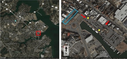
(A) Annapolis, located adjacent to the Chesapeake Bay. The red box marks the historic downtown and City Dock area. (B) Aerial image of the City Dock parking lot, with the locations of two storm drains marked in yellow and two entrances marked with red arrows. The blue rectangle marks the Market Space parking lot.

Incidence of high-tide flooding

Annapolis has a nuisance flood threshold that is intended to represent the water level at which disruptive effects materialize. The current threshold is 2.6 feet above mean lower low water, equal to 1.83 feet above NAVD88 (the North American Vertical Datum of 1988), which is used as the reference hereafter (25). In May 2018, the threshold was changed from 1.63 to 1.83 feet. While the nuisance flood threshold is a useful guide, the criteria for selecting this threshold are not well defined, and the effect of rainfall on flood incidence in this location is uncertain. Therefore, we identify a flooding threshold based on the documentation of flooding combined with tide gauge, rainfall, and elevation data.

We gathered 50 photographs of flooding at City Dock across 19 days in 2016 and 2017 from local government sources and social media (see Materials and Methods). Days with and without documented flooding are plotted on the basis of the maximum hourly water level and total precipitation in Fig. 2. It is not expected that every flood will be documented, so the gray dots represent either days with no flooding or days with flooding that was not documented (additional analysis of flood documentation patterns is provided in fig. S1). Nonetheless, we are able to use the photos to confirm that flooding at City Dock is frequently driven by water level, rather than rainfall, and then to empirically verify the water-level threshold at which flooding begins. The occurrence of tidal flooding in the absence of precipitation is demonstrated by the numerous days with documented flooding without any precipitation in the top left quadrant of Fig. 2. The estimated flood threshold is further informed by video footage of City Dock covering 1 March 2018 to 7 March 2018 (as the City of Annapolis only stores video footage for a few weeks, it was not possible to obtain footage for the entire time period of interest). During the initial rise in water levels, the video footage reveals a very small pool of water at 1.71 feet and a substantial pool at 1.74 feet. On the basis of the photographic and video evidence, we set the flood threshold at 1.73 feet for our analysis. This observation-based threshold is halfway between the current nuisance flood threshold (1.83 feet) and the former (1.63 feet).

Fig. 2. Flood documentation as a function of maximum daily water level and total daily rainfall.

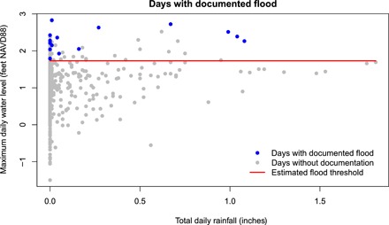
For each day in 2016 and 2017, the maximum daily water level and total daily rainfall are plotted. A day is considered documented if there is photographic documentation of flooding on that day. Days with a photograph of flooding are plotted as blue dots, while days without a photograph of flooding are plotted as gray dots. The concentration of flood days with zero rainfall (in the upper left corner) demonstrates that high water levels alone can cause flooding.

The relationship between the water level recorded at the tide gauge and flooding in the parking lot differs based on whether the water level is rising or falling. Once water has accumulated, it persists after the water level has receded below 1.73 feet. The rate at which the flooding in the parking lot recedes likely is affected by how quickly the water level is dropping and how low it ultimately falls. As discussed later, we account for this explicitly when estimating how floods affect local economic activity.

To account for different flood severities, we define three categories of flood events: minor (1.73 to 2.03 feet), moderate (2.03 to 2.33 feet), and major (>2.33 feet). The levels are set on the basis of the degree of disruption to parking lot operation and differ from the National Weather Service’s flood category definitions. The flood extent associated with the lower limit of each category is approximated in Fig. 3 using elevation data, and we provide photographs of each type of flood in fig. S2 for comparison. At minor flood levels, the south side of the main parking lot is submerged, but the north side remains passable. At moderate flood levels, the north side of the lot and the main entrance begin to flood. Last, at major flood levels, the rear entrance also becomes inaccessible. In 2016 and 2017, the peak hourly water level recorded was 2.832 feet. Even at that level, the rear portion of the lot (in the bottom-right corner of the image) remains dry, so parking is possible if cars drive through the flooded entrances.

Fig. 3. High-tide flood extent at water levels of 1.73, 2.03, 2.33, and 2.83 feet (the maximum observed water level in our data) based on LiDAR (light detection and ranging) data.

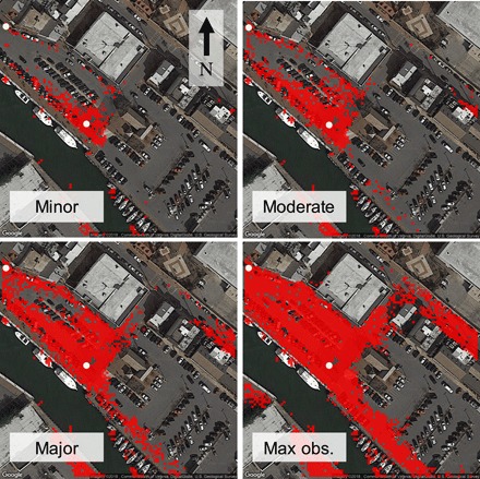
See Materials and Methods for additional documentation. Corresponding flood categories are specified in the first three images, and the fourth image depicts the maximum water level observed in our data, 2.83 feet. Points are aggregated to 5 feet by 5 feet cells, and cells are shaded red if the minimum elevation within the cell is lower than the specified water level. Storm drains are marked in yellow.

Hourly flood impacts on local economic activity

To discern the impacts of high-tide flooding on local economic activity, we use a fixed-effects regression, an econometric technique widely used to identify the impacts of temperature and other climate variables on societal outcomes (26, 27). We adapt this approach to estimate the impacts of high-tide flooding on local economic activity using visits to City Dock as our primary outcome. Our approach isolates the impact of floods on visits by flexibly accounting for typical patterns in both flooding and visitation.

We obtained individual records of parking transactions in the City Dock parking lot from May 2016 to November 2017 and summed them to an hourly level. We then match each hour to hourly tidal and precipitation data. Here, we refer to each parking transaction as a “visit,” recognizing that each car parked may entail more than one visitor and that not all visitors park at City Dock. Each hour is assigned to either no flood, minor flood, moderate flood, or major flood based on the recorded water level. The effect of flooding on visits is estimated by regressing the number of visits in an hour on the presence of different levels of flooding. Since visits are a count variable, Poisson and negative binomial models are used. We control for potential confounders that are correlated with both flood incidence and visits to isolate the effect of flooding. Fixed effects for each month, day of week, and time of day account for routine variation in visits to this downtown business district. The hour effects control for differences in visitation patterns throughout the day (for example, people visit in the evening more often than the afternoon), day effects control for weekly cycles (for example, people are more likely to visit on the weekends), and month effects control for seasonality in visitation and flooding. Because precipitation is known to affect consumer behavior and it may be seasonally correlated with high-tide flooding, we also include precipitation in the regression (28, 29). With these control variables, we are identifying the effect of floods by comparing visits during flood hours to visits during other hours at the same time of day, on the same day of the week, in the same month after controlling for the effect of rainfall on visits.

Hourly visits (V_hdwm) are modeled as follows

$$\begin{array}{cc}\hfill \text{log}({\mathit{V}}_{\mathit{h}\mathit{d}\mathit{w}\mathit{m}})=& {\mathrm{\beta }}_1{\mathit{Minor}}_{\mathit{h}\mathit{d}\mathit{w}\mathit{m}}+{\mathrm{\beta }}_2{\mathit{Moderate}}_{\mathit{h}\mathit{d}\mathit{w}\mathit{m}}+{\mathrm{\beta }}_3{\mathit{Major}}_{\mathit{h}\mathit{d}\mathit{w}\mathit{m}}+\hfill \\ & {\mathrm{\beta }}_4{\mathit{Precip}}_{\mathit{h}\mathit{d}\mathit{w}\mathit{m}}+{\mathrm{\alpha }}_{\mathit{h}}+{\mathrm{\lambda }}_{\mathit{d}}+{\mathrm{\gamma }}_{\mathit{m}}+{\mathrm{\epsilon }}_{\mathit{h}\mathit{d}\mathit{w}\mathit{m}}\hfill \end{array}$$ (1)

Minor, Moderate, and Major are binary variables equal to 1 if that hour h in day d of week w of month m is a flood of the given severity, and 0 otherwise. Precipitation is included as a continuous variable of total inches in the hour. α_h, λ_d, and γ_m are dummy variables for the hour of day, day of week, and month, respectively. The coefficients of interest are β₁, β₂, and β₃, which represent the change in visits due to the presence of minor, moderate, and major flooding, respectively. The model estimates these effects relative to a “no flood” baseline condition.

We then run the same model with lagged flood variables. Including the lags enables us to capture potential residual flooding as the water is receding and temporal displacement of transactions (i.e., if people who are dissuaded by flooding simply come later in the day or the day after)

$$\begin{array}{cc}\hfill \text{log}({\mathit{V}}_{\mathit{h}\mathit{d}\mathit{w}\mathit{m}})=& {\mathrm{\beta }}_1{\mathit{Minor}}_{\mathit{h}\mathit{d}\mathit{w}\mathit{m}}+{\mathrm{\beta }}_2{\mathit{Moderate}}_{\mathit{h}\mathit{d}\mathit{w}\mathit{m}}+{\mathrm{\beta }}_3{\mathit{Major}}_{\mathit{h}\mathit{d}\mathit{w}\mathit{m}}+\hfill \\ & {\mathrm{\beta }}_4{\mathit{Precip}}_{\mathit{h}\mathit{d}\mathit{w}\mathit{m}}+{\mathrm{\alpha }}_{\mathit{h}}+{\mathrm{\lambda }}_{\mathit{d}}+{\mathrm{\gamma }}_{\mathit{m}}+{\mathrm{\delta }}_1\mathit{PostHour}{\mathit{1}}_{\mathit{h}\mathit{d}\mathit{w}\mathit{m}}+\hfill \\ & {\mathrm{\delta }}_2\mathit{PostHour}{\mathit{2}}_{\mathit{h}\mathit{d}\mathit{w}\mathit{m}}+{\mathrm{\delta }}_3\mathit{PostHour}{\mathit{3}}_{\mathit{h}\mathit{d}\mathit{w}\mathit{m}}+\hfill \\ & {\mathrm{\delta }}_4\mathit{PostHour}{\mathit{4}}_{\mathit{h}\mathit{d}\mathit{w}\mathit{m}}+{\mathrm{\delta }}_5\mathit{PostHour}{\mathit{5}}_{\mathit{h}\mathit{d}\mathit{w}\mathit{m}}+\hfill \\ & {\mathrm{\delta }}_6\mathit{PostHour}{\mathit{6}}_{\mathit{h}\mathit{d}\mathit{w}\mathit{m}}+{\mathrm{\delta }}_7\mathit{PostDay}{\mathit{1}}_{\mathit{h}\mathit{d}\mathit{w}\mathit{m}}+{\mathrm{\epsilon }}_{\mathit{h}\mathit{d}\mathit{w}\mathit{m}}\hfill \end{array}$$ (2)

We include lagged flood variables for 6 hours after the flood (PostHour). PostHour1 takes a value of 1 for the hour after the water level drops below the flood threshold and is 0 otherwise; PostHour2 equals 1 in the second hour after the water level drops below the flood threshold, and so forth. We also include a lagged day variable (PostDay), which equals 1 for hours on the day immediately following a day with a flood and is 0 otherwise. The lags are set to zero if the hour coincides with a flood hour; that is, a given hour cannot be both a flood hour and a lagged flood hour. The results from additional specifications, using water level as a continuous variable and using a binary flood/no flood variable, are given in the Supplementary Materials.

The results of the Poisson and negative binomial models are shown in Fig. 4. All four models produce similar results: Minor floods reduce visits by 37 to 38%, moderate floods by 63 to 65%, and major floods by 88 to 89%. As expected, precipitation has a negative effect as well: An average hour of rain (0.085 inches) reduces visits by 11 to 15%. By controlling explicitly for rainfall and confirming its negative effect, we increase confidence that the effect we are measuring is indeed due to high-tide flooding, separate from the independent effects of precipitation.

Fig. 4. Estimated changes in visits due to high-tide flooding for minor, moderate, and major flood hours; during rain hours; and during postflood time periods (1 to 6 hours postflood and the day after a flood).

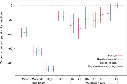
Errors bars indicate 95% confidence intervals using standard errors for the negative binomial models and robust standard errors for the Poisson models. Effect of rainfall is represented as the effect of 0.085 inches/hour, which is the average rainfall in an hour during hours with rain.

As floods become more severe, visits fall further, as expected. Notably, the estimated percentage losses for minor, moderate, and major high-tide flooding exceed the share of parking spots inundated at those flood levels. Although minor flooding inundates a maximum of 28 parking spaces (15% of total available spaces), 36% fewer visits occur during minor flood hours as compared with the same time of day, day of week, and month without flooding. The comparatively large decline in visits may result from people not knowing whether the tide is rising or receding and choosing to park elsewhere altogether. According to interviewees (table S1), cars often experience exterior and interior water damage, including to their engines, during these events. Although the floodwater is brackish, it can still cause substantial damage to vehicles. In some cases, the police block off the flooded area with a yellow barricade, which may dissuade visitors from using the lot even if many other spots are not blocked. The 63% decline in visits during moderate flood hours may occur because the primary entrance can be flooded, so only those who know to drive around to the side entrance are able to park. Last, at major flood stage, visits almost completely stop. The few remaining transactions are all for the back part of the lot, which is still dry.

The right-hand side of Fig. 4 shows the lagged effects of flooding. These estimates indicate that there is a sustained decline in visits well after the water level recedes below the flood threshold of 1.73 feet. The effects are statistically significant (95% confidence intervals do not cross zero) for a full 5 hours following a flood event, even though the estimates are noisier than those of the direct flood effects. Postflood effects wane as time passes: In the hour right after a flood event, visits are reduced by 26 to 28%, but this effect shrinks to 13 to 14% in the fifth hour after a flood. We find no evidence that visits increase on days that follow floods.

These postflood effects likely arise from a combination of behavioral and physical factors. We discuss two potential explanations here. First, as noted above, the video footage shows that a pool of water can persist well after the water level drops below the flood threshold. Therefore, we may be observing the effects of residual flooding during these hours immediately after the water level drops below the flood threshold. Second, human factors may drive this extended effect as well: Barriers around the flooded area may not be taken down promptly, or people may hear that City Dock is flooded without knowing if or when the flooding has dissipated (announcements of high-tide flooding are disseminated through the city’s social media accounts and roadside signage). Another possibility is that certain businesses close for the entire day if there is flooding in the morning, so there is less reason to park at the City Dock parking lot. However, on the basis of our interviews and review of social media, we identified only one of the 16 businesses at City Dock that closes during these events (additional description of interviews is available in table S1). Most are at sufficient elevation that water does not enter their location and remain open regardless of the parking lot’s accessibility. The lack of a rebound effect the next day may be due to the fact that many of the businesses are restaurants or retail, so people substitute spatially (with restaurants and stores in other locations) rather than temporally (coming the next day).

To investigate the possibility of spatial substitution, parking transaction data from the nearest alternative parking lot, Market Space, were acquired. The Market Space lot, marked with a blue rectangle in Fig. 1B, is located across the street from City Dock; however, it is several feet higher and does not experience flooding during high-tide flood events. Using the exact same models, but substituting Market Space visits for City Dock visits, we find no effect of City Dock flooding on Market Space visits (fig. S4). The results imply that, if the revenue from would-be City Dock visitors is being recouped at all, then it is not in the proximate downtown area.

Cumulative flood impacts on local economic activity

Building on the results from the regression analysis, we calculate the cumulative annual impact of high-tide flooding by comparing observed visits to estimated visits in a counterfactual scenario in which no flooding occurs. We also project how this cumulative impact is likely to change as sea level continues to rise.

First, to enable estimation on an annual timeframe, we impute parking transaction data for time periods in 2017 that lack parking records, chiefly the month of December (see Materials and Methods). Then, to estimate how many visitors would have come to City Dock in the counterfactual scenario of no flooding, we “undo” the impact of flooding for each affected hour in 2017 using the percentage losses from the regression analysis. If an hour in 2017 experienced minor flooding, and minor flooding decreases visits by 37.5%, then the number of visits we observe is 100% – 37.5% = 62.5% of what visits would have been had there been no flooding. This calculation yields the central estimate for the number of visits in the no flood condition, and we repeat the same calculation with the coefficient’s upper bound and lower bound to obtain a 95% confidence interval for the counterfactual number of visits. Then, we repeat this process for each hour in 2017 that is affected by minor, moderate, or major flooding, as well as the six postflood lag hours. This calculation gives us a number of visits for each hour in the year under a no flood condition and the surrounding confidence interval. Last, we sum the no flood annual visits and compare them to the observed visits to calculate the total impact of high-tide flooding on visits. In 2017, high-tide flooding led to the loss of 2916 visitors to City Dock (a 1.7% decrease), with a 95% confidence interval of 1667 to 4378 (1.0 to 2.6%). Note that this estimation method only modifies the water levels to undo the effect of the flood on visits. Other factors that are in the model and affect visits, such as the day of the week, rainfall, or time of day, are not altered.

In addition, rather than removing all of the flooding, we can adjust the mean sea level up and down to examine how the impact of high-tide floods has changed over time (see Materials and Methods). Mean sea level has risen almost 1 foot in Annapolis since 1950 (Fig. 5A). This rise has led to a nonlinear increase in the number of flood hours during the parking lot’s operational hours, as shown in Fig. 5B. To see how this historical increase in sea level has affected visits, we first calculate the difference between the mean sea level in 2017 and the mean sea level in the previous year of interest. Then, we adjust all observed water levels in 2017 by that fixed amount to arrive at a counterfactual water level. Minor, moderate, major, and lag hours for flooding are reassigned on the basis of these water levels. Then, a counterfactual number of visits are estimated through a similar “undoing” process as described above. We sum the counterfactual visits to arrive at an annual number of visits under the previous year’s mean sea level. The results of this analysis are shown in the inset of Fig. 5C.

Fig. 5. Cumulative impacts of high-tide flooding on visits to City Dock, as observed to date and projected under additional sea level rise.

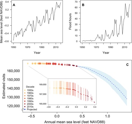
(A) Annual mean sea level (feet NAVD88) over time in Annapolis (NOAA tide gauge #8575512). (B) Hours above the high-tide flood threshold each year. Only hours in which Annapolis City Dock parking lot is operational are included. (C) Cumulative impacts of high-tide flooding on visits to City Dock based on mean annual sea level. Estimates are based on a uniform increase or decrease compared with 2017 water levels, holding all else constant. Error bars mark 95% confidence intervals. For observed mean sea levels, each point represents 1 year, with color reflecting the decade in which the sea level was observed. Higher sea levels and associated visits are projected in blue. Note that a maximum of one additional foot of sea level rise is included in this plot; 1 foot is the lower bound of projected global mean sea level rise for the 21st century. The high and extreme sea level rise scenarios are 6.6 and 8.2 feet, respectively (1).

Last, we shift sea level up to project how the impacts of high-tide flooding are likely to evolve. Using an identical procedure as for the historical mean sea levels, we increase sea level by up to 1 foot higher than 2017 observed water levels. The resulting blue curve in Fig. 5C demonstrates that visits to City Dock drop steeply as sea level rises. Projections indicate that with three additional inches of sea level rise, an additional 3221 visits (95% confidence interval, 1019 to 5084) would be lost. These additional inches of sea level rise could occur within two decades at current rates of sea level change. With 1 foot of additional sea level rise, City Dock would lose 37,506 more visits (28,098 to 45,559) due to high-tide flooding. This is equivalent to a 24% (19 to 28%) decrease relative to a year with no floods.

These projections assume that the relationship between water levels and visits remains constant over time; they do not account for potential adaptations or changes that could occur in the future. By capturing only current adaptation levels, the projections demonstrate the potential value of future adaptation measures. There are a number of potential adaptations that would alter future impacts, such as the local government investing in engineering solutions, businesses adjusting operating hours, and visitors planning around high-tide hours. However, as in many contexts, adaptation will be constrained by a variety of technical, financial, behavioral, and political factors.

Revenue losses from high-tide flooding

Last, we estimate losses in revenue that may have resulted from decreased customer access due to high-tide flooding in Annapolis. The 16 most proximate businesses to City Dock comprise $12.2 million in annual revenue (30). The amount of revenue lost depends on the relationship between cars parking at City Dock and sales, as well as how revenue per visit may change from hour to hour or month to month. Given limited data on business revenues, we provide a range of estimates. The City of Annapolis gathered daily revenue data from eight flood-affected businesses, comparing revenue on a flood date to the same day in previous years (31). The flood events examined in their analysis overlap mostly with our major flood category, with a few events falling into our moderate category. They find that revenue decreased on average 22.5% between flood days and the same date in previous years. For comparison, our data indicate that on days when there was at least 1 hour of moderate flooding, visits decreased by an average of 37%, implying that a 1% loss in visits translated to a 0.61% loss in revenue. We adopt a range around this 0.61% figure and assume that a 1% loss in visits leads to a 0.4 to 0.8% loss in revenue. Under these assumptions, City Dock businesses lost $86,000 to $172,000 in 2017 due to high-tide flooding, equivalent to 0.7 to 1.4% of their annual revenue.

The estimate of lost revenue represents only losses to the stores in the immediate vicinity of the City Dock lot. We find no evidence of customers coming at other times or parking at the closest alternative lot, but it is possible that they choose locations farther away. If businesses elsewhere experience an increase in visits when City Dock is flooded, the net loss for local revenue would be lower than these figures.

CONCLUSIONS

This analysis empirically estimates local business disruption due to high-tide flooding. High-tide flooding already measurably reduces visits to City Dock in Annapolis, Maryland. Decreased visits persist for hours after the water recedes. The cumulative impacts amount to a loss of about 3000 visits in 2017, equal to a 1.7% loss. Visits decrease increasingly rapidly as sea level rises; with 1 foot of additional sea level rise, City Dock would see 24% fewer visitors than in a year without high-tide flooding. Although potential City Dock customers may be spending money in other locations, we find no evidence that visits are recovered later in time or at the closest alternative parking lot. Therefore, the losses due to recurrent flooding are already affecting the profitability of these businesses, and the losses will worsen as sea level rises unless changes are made.

Our analysis comprises one component of losses due to high-tide flooding. Additional research is needed to explore the full range of impacts, such as increased travel time due to road closures, missed work hours, or damage to cars, roadways, or other infrastructure. A more comprehensive understanding of local impacts will help guide investments in drainage infrastructure, pumps, and structure elevation. Last, as a cost of climate change, these emerging sea level rise impacts can inform efforts to mitigate greenhouse gas emissions and limit future sea level rise.

MATERIALS AND METHODS

Flood incidence

We assembled the documentation of flooding at City Dock for 2016 and 2017 from multiple sources. Officials from the Annapolis Office of Emergency Management and the Annapolis Department of Public Works shared dated photographs. Public Twitter and Facebook posts and photos were also assembled. First, for City Dock businesses with social media accounts, we examined their public history and flagged any content that depicted flooding. We also searched for the hashtags “#nuisanceflooding” and “#dockstreet” on Twitter from 2016 to 2017 and extracted photos that showed water on City Dock from the search results. For the photographs from social media, the date and time of posting were recorded.

Hourly tide gauge measurements are from NOAA National Ocean Service/Center for Operational Oceanographic Products and Services tide gauge #8575512 located in the U.S. Naval Academy Hendrix Oceanography Lab. The source of the precipitation data is the KNAK Automated Surface Observing Systems weather station. Both stations are located along the Severn River and are within 0.75 miles of each other. We matched the dates and times of the photographs to tide heights and precipitation to assess the influence of water level and rainfall on flood incidence.

To produce Fig. 3, we obtained light detection and ranging (LiDAR) data for this area from MD iMAP. These data from 2011 meet USGS (United States Geological Survey) LiDAR base specification 1.3 with a vertical position accuracy of 15-cm root mean square error. Full documentation is available at https://imap.maryland.gov/Pages/lidar-metadata.aspx.

Parking transactions

Visitors to the City Dock parking lot and the Market Space parking lot are required to pay for parking from 10:00 a.m. to 7:30 p.m. Monday to Saturday and 12:00 p.m. to 7:30 p.m. on Sunday. Parking is limited to a maximum of 2 hours per visit. Payment is not enforced from the week of Thanksgiving through New Year’s Day, and the lot is closed for 2 weeks in October for the annual boat show. In addition, due to a construction project on the dock, the City Dock lot was closed from January to May 2016. Data include individual transactions with a timestamp and pay station code indicating the location of the transaction.

The data used in the regression included only hours with a number of visits, water level, and rainfall measurement. Summary statistics of the key variables used in the regression are shown in Table 1. All analyses were performed using R. The raw data and the code are available at https://purl.stanford.edu/td717bf3410.

Table 1. Summary statistics of key variables.

Total observations (hours) in data = 4584.

Variable	Mean	Min	Max
Water level (feet NAVD88)	0.406	−2.13	2.59
Visits per hour	52.60	0	120
Rainfall (inches)	0.005	0	1.03
Flood*	0.020	0	1
Minor flood*	0.011	0	1
Moderate flood*	0.007	0	1
Major flood*	0.002	0	1
First hour postflood*	0.004	0	1
Second hour postflood*	0.005	0	1
Third hour postflood*	0.006	0	1
Fourth hour postflood*	0.006	0	1
Fifth hour postflood*	0.006	0	1
Sixth hour postflood*	0.007	0	1
Day after flood*	0.089	0	1

*Binary variables.

To calculate the lost visits on an annual basis, we made several adjustments to the dataset. First, hours with water level measurements but without rainfall measurements were added back to the dataset since rainfall is not used in the calculation of lost visits. Second, parking data were imputed for missing hours as payment is not required for parking during the time period from Thanksgiving to New Year’s Day. The number of transactions was imputed for 1 January, 2 January, and the last week of November based on the month, day of week, and hour. Transactions for the month of December were imputed on the basis of the day of week and hour using November data. There were no flood hours in either November 2016 or November 2017, so the mean number of transactions observed at 2:00 p.m. on Tuesdays in November is assigned as the number of no flood visits to all 2:00 p.m. on Tuesdays in December and so forth. This resulted in a calendar year of transactions and flood levels that served as the basis of our estimates of lost visits (this dataset omits 2 weeks in October, during which the parking lot is closed for the annual boat show, and a shuttle brings visitors to the area).

Counterfactual estimation

To calculate visits under counterfactual scenarios with different sea levels, we adjusted the observed hourly water levels uniformly by the corresponding amount of sea level change. Using the same flood thresholds, hours were assigned using these adjusted water levels to minor, moderate, and major flooding. Postflood hours were also reassigned. Hours can be postflood lag hours due to floods that occur outside of the parking lot’s operational hours; for example, if the water level recedes below the flood threshold at 8:00 a.m. (before the parking lot requires payment), 10:00 a.m. would be marked as the second hour postflood.

The estimate of the counterfactual number of visits is based on the parameters from Eq. 2. For example, if we observe 100 visits in a moderate flood hour and that hour experiences no flooding in the counterfactual scenario, and then if moderate flooding reduces visits by 50%, we estimated that 100/(1 − 0.5) = 200 visits would have occurred absent any flooding. The confidence intervals depend on the observed and counterfactual states. If no change occurs, for example, an observed minor flood hour remains a minor flood in the counterfactual, then this figure is known with certainty. If an hour changes conditions, then the confidence interval on the percentage loss estimate (as shown in Fig. 4) is used to recover a 95% confidence interval for the number of visits. Repeating the regression in Eq. 2 with different omitted categories enabled conversion to and from all pairs of observed and counterfactual conditions. For example, by including a variable for “no condition” and omitting the “moderate” variable, a coefficient and confidence interval can be obtained for hours that are observed as moderate flood hours and change to other conditions. There are 2 hours in the data with zero observed transactions; these remain as zero transactions under all conditions. We repeat the calculation converting observed to counterfactual conditions for each hour in our data representing the 2017 calendar year. Then, we sum the number of visits in the counterfactual and compare it to the 2017 observed visits.

Revenue losses

We acquired annual revenue data from the Reference USA database for 17 businesses located on Prince George Street, Craig Street, and Dock Street—businesses for which we expect City Dock to be the primary parking area (30). One business was removed because it no longer exists at the City Dock location. The sum of the revenue of these 16 businesses was $12.2 million. We estimated the revenue lost due to high-tide flooding using two different parameters: A lower bound of a 0.4% loss in revenue for every 1% loss in visitors, and an upper bound of a 0.8% loss in revenue for every 1% loss in visitors. We combined these parameters with our estimated loss in visitors and the total revenue figure to estimate the revenue losses.

SUPPLEMENTARY MATERIALS

Supplementary material for this article is available at http://advances.sciencemag.org/cgi/content/full/5/2/eaau2736/DC1

Supplementary Material

Table S1. Summary of interviews.

Table S2. Regression results for model specifications.

Table S3. Regression results for alternative specifications.

Fig. S1. Documentation of flooding by time of day and by water level.

Fig. S2. Documentation of flooding on City Dock.

Fig. S3. Visits as a continuous function of water level.

Fig. S4. Model results showing estimated changes in visits to the Market Space parking lot during minor, moderate, or major flood hours; during rain hours; and during postflood time periods (1 to 6 hours postflood and the day after a flood).

Fig. S5. Estimated visits in past years using hourly water level measurements.

References (32–36)

REFERENCES AND NOTES

- 1.W. V Sweet, R. Horton, R. E. Kopp, A. N. LeGrande, A. Romanou, in Climate Science Special Report: Fourth National Climate Assessment, Volume I, D. J. Wuebbles, D. W. Fahey, K. A. Hibbard, D. J. Dokken, B. C. Stewart, T. K. Maycock, Eds. (U.S. Global Change Research Program, USA, 2017), pp. 333–363. [Google Scholar]
- 2.J. A. Church, P. U. Clark, A. Cazenave, J. M. Gregory, S. Jevrejeva, A. Levermann, M. A. Merrifield, G. A. Milne, R. S. Nerem, P. D. Nunn, A. J. Payne, W. T. Pfeffer, D. Stammer, A. S. Unnikrishnan, in Climate Change 2013: The Physical Science Basis. Contribution of Working Group I to the Fifth Assessment Report of the Intergovernmental Panel on Climate Change, T. F. Stocker, D. Qin, G.-K. Plattner, M. Tignor, S. K. Allen, J. Boschung, A. Nauels, Y. Xia, V. Bex, P. M. Midgley, Eds. (Cambridge Univ. Press, 2013); www.ipcc.ch/pdf/assessment-report/ar5/wg1/WG1AR5_Chapter13_FINAL.pdf).
- 3.Nicholls R. J., Hoozemans F. M. J., Marchand M., Increasing flood risk and wetland losses due to global sea-level rise: Regional and global analyses. Glob. Environ. Chang. 9, S69–S87 (1999). [Google Scholar]
- 4.Hinkel J., Lincke D., Vafeidis A. T., Perrette M., Nicholls R. J., Tol R. S. J., Marzeion B., Fettweis X., Ionescu C., Levermann A., Coastal flood damage and adaptation costs under 21st century sea-level rise. Proc. Natl. Acad. Sci. U.S.A. 111, 3292–3297 (2014). [DOI] [PMC free article] [PubMed] [Google Scholar]
- 5.Tebaldi C., Strauss B. H., Zervas C. E., Modelling sea level rise impacts on storm surges along US coasts. Environ. Res. Lett. 7, 014032 (2012). [Google Scholar]
- 6.Hsiang S., Kopp R., Jina A., Rising J., Delgado M., Mohan S., Rasmussen D. J., Muir-Wood R., Wilson P., Oppenheimer M., Larsen K., Houser T., Estimating economic damage from climate change in the United States. Science 356, 1362–1369 (2017). [DOI] [PubMed] [Google Scholar]
- 7.Hallegatte S., Green C., Nicholls R. J., Corfee-Morlot J., Future flood losses in major coastal cities. Nat. Clim. Chang. 3, 802–806 (2013). [Google Scholar]
- 8.Dahl K. A., Fitzpatrick M. F., Spanger-Siegfried E., Sea level rise drives increased tidal flooding frequency at tide gauges along the U.S. East and Gulf Coasts: Projections for 2030 and 2045. PLOS ONE 12, e0170949 (2017). [DOI] [PMC free article] [PubMed] [Google Scholar]
- 9.W. V Sweet, G. Dusek, J. Obeysekera, J. J. Marra, Patterns and projections of high tide flooding along the U.S. coastline using a common impact threshold (2018); https://tidesandcurrents.noaa.gov/publications/techrpt86_PaP_of_HTFlooding.pdf.
- 10.Wdowinski S., Bray R., Kirtman B. P., Wu Z., Increasing flooding hazard in coastal communities due to rising sea level: Case study of Miami Beach, Florida. Ocean Coast. Manag. 126, 1–8 (2016). [Google Scholar]
- 11.Flood J. F., Cahoon L. B., Risks to coastal wastewater collection systems from sea-level rise and climate change. J. Coast. Res. 27, 652–660 (2011). [Google Scholar]
- 12.Sweet W. V., Park J., From the extreme to the mean: Acceleration and tipping points of coastal inundation from sea level rise. Earth’s Future 2, 579–600 (2014). [Google Scholar]
- 13.Union of Concerned Scientists, When Rising Seas Hit Home (2017).
- 14.Hammond M. J., Chen A. S., Djordjević S., Butler D., Mark O., Urban flood impact assessment: A state-of-the-art review. Urban Water J. 14–29 (2013). [Google Scholar]
- 15.F. Messner, E. Penning-Rowsell, C. Green, V. Meyer, S. Tunstall, A. van der Veen, Evaluating flood damages: guidance and recommendations on principles and methods (2007); www.floodsite.net/html/partner_area/project_docs/T09_06_01_Flood_damage_guidelines_D9_1_v2_2_p44.pdf.
- 16.Merz B., Kreibich H., Schwarze R., Thieken A., Review article “Assessment of economic flood damage”. Nat. Hazards Earth Syst. Sci. 10, 1697–1724 (2010). [Google Scholar]
- 17.I. Seifert, H. Kreibich, B. Merz, A. Thieken, in Flood Risk Management: Research and Practice, P. Samuels, S. Huntington, W. Allsop, J. Harrop, Eds. (Taylor & Francis Group, 2009), pp. 1669–1675. [Google Scholar]
- 18.Hallegatte S., An adaptive regional input-output model and its application to the assessment of the economic cost of Katrina. Risk Anal. 28, 779–799 (2008). [DOI] [PubMed] [Google Scholar]
- 19.Ranger N., Hallegatte S., Bhattacharya S., Bachu M., Priya S., Dhore K., Rafique F., Mathur P., Naville N., Henriet F., Herweijer C., Pohit S., Corfee-Morlot J., An assessment of the potential impact of climate change on flood risk in Mumbai. Clim. Change 104, 139–167 (2011). [Google Scholar]
- 20.Rose A., Porter K., Dash N., Bouabid J., Huyck C., Whitehead J., Shaw D., Eguchi R., Taylor C., McLane T., Tobin L. T., Ganderton P. T., Godschalk D., Kiremidjian A. S., Tierney K., West C. T., Benefit-cost analysis of FEMA hazard mitigation grants. Nat. Hazards Rev. 8, 97–111 (2007). [Google Scholar]
- 21.Moftakhari H. R., AghaKouchak A., Sanders B. F., Matthew R. A., Cumulative hazard: The case of nuisance flooding. Earth’s Future 5, 214–223 (2017). [Google Scholar]
- 22.Sadler J. M., Haselden N., Mellon K., Hackel A., Son V., Mayfield J., Blase A., Goodall J. L., Impact of sea-level rise on roadway flooding in the Hampton Roads region, Virginia. J. Infrastruct. Syst. 23, 05017006 (2017). [Google Scholar]
- 23.Sallenger A. H. Jr., Doran K. S., Howd P. A., Hotspot of accelerated sea-level rise on the Atlantic coast of North America. Nat. Clim. Chang. 2, 884–888 (2012). [Google Scholar]
- 24.Ezer T., Corlett W. B., Is sea level rise accelerating in the Chesapeake Bay? A demonstration of a novel new approach for analyzing sea level data. Geophys. Res. Lett. 39, L19605 (2012). [Google Scholar]
- 25.Datums for 8575512, Annapolis MD; https://tidesandcurrents.noaa.gov/datums.html?id=8575512.
- 26.Carleton T. A., Hsiang S. M., Social and economic impacts of climate. Science 353, aad9837 (2016). [DOI] [PubMed] [Google Scholar]
- 27.Dell M., Jones B. F., Olken B. A., What do we learn from the weather ? The New Climate–Economy Literature. J. Econ. Lit. 52, 740–798 (2014). [Google Scholar]
- 28.M. Starr-McCluer, “The effects of weather on retail sales” (FEDS Working Paper no. 2000-08, 2000); https://ssrn.com/abstract=221728.
- 29.S. Agarwal, J. B. Jensen, F. Monte, “The geography of consumption” (NBER Working Paper no. 23616, 2017); 10.3386/w23616.
- 30.InfoGroup, Reference USA Company Profiles (2018).
- 31.City of Annapolis, “State of Maryland Hazard Mitigation Grant Program Application” (2017).
- 32.Davis J. L., Mitrovica J. X., Glacial isostatic adjustment and the anomalous tide gauge record of eastern North America. Nature 379, 331–333 (1996). [Google Scholar]
- 33.Ezer T., Atkinson L. P., Corlett W. B., Blanco J. L., Gulf Stream’s induced sea level rise and variability along the U.S. mid-Atlantic coast. J. Geophys. Res. Oceans 118, 685–697 (2013). [Google Scholar]
- 34.Srokosz M., Baringer M., Bryden H., Cunningham S., Delworth T., Lozier S., Marotzke J., Sutton R., Past, present, and future changes in the Atlantic Meridional Overturning Circulation. Bull. Am. Meteorol. Soc. 93, 1663–1676 (2012). [Google Scholar]
- 35.Boon J. D., Evidence of sea level acceleration at U.S. and Canadian tide stations, Atlantic coast, North America. J. Coast. Res. 28, 1437–1445 (2012). [Google Scholar]
- 36.Ezer T., Atkinson L. P., Accelerated flooding along the U.S. East Coast: On the impact of sea-level rise, tides, storms, the Gulf Stream, and the North Atlantic Oscillations. Earth’s Future 2, 362–382 (2014). [Google Scholar]
Associated Data
This section collects any data citations, data availability statements, or supplementary materials included in this article.