Region-segmentation strategy for Bruch’s membrane opening detection in spectral domain optical coherence tomography images

Abstract

Bruch’s membrane opening (BMO) is an important biomarker in the progression of glaucoma. Bruch’s membrane opening minimum rim width (BMO-MRW), cup-to-disc ratio in spectral domain optical coherence tomography (SD-OCT) and lamina cribrosa depth based on BMO are important measurable parameters for glaucoma diagnosis. The accuracy of measuring these parameters is significantly affected by BMO detection. In this paper, we propose a method for automatically detecting BMO in SD-OCT volumes accurately to reduce the impact of the border tissue and vessel shadows. The method includes three stages: a coarse detection stage composed by retinal pigment epithelium layer segmentation, optic disc segmentation, and multi-modal registration; a fixed detection stage based on the U-net in which BMO detection is transformed into a region segmentation problem and an area bias component is proposed in the loss function; and a post-processing stage based on the consistency of results to remove outliers. Experimental results show that the proposed method outperforms previous methods and achieves a mean error of 42.38 μm.

1. Introduction

Glaucoma is an irreversible, progressive optic neuropathy that causes nerve fiber damage, visual loss, and even blindness [1, 2]. Early detection and treatment can slow the progression of the disease; thus, identification of the structural changes in early glaucoma, such as cup-to-disc ratio and retinal nerve fiber layer (RNFL) thickness, is important [3, 4].

Bruch’s membrane opening (BMO) or neural canal opening, which remains stable with the progression of glaucoma, is an important biomarker in the optic nerve head (ONH) in Spectral-Domain Optical Coherence Tomography (SD-OCT) [5]. It is defined as the termination of the retinal pigment epithelium (RPE) layer. As introduced in [6], the BMO points in SD-OCT represent the true position of the optic disc. Thus, the disc margin can also be identified by aligning the color fundus image and the SD-OCT volumes.

Bruch’s membrane opening minimum rim width (BMO-MRW), defined as the minimum Euclidean distance from BMO to the internal limiting membrane surface, performs better in early glaucoma diagnosis than other structure parameters, such as RNFL thickness [7]. Moreover, BMO plays an indispensable role in lamina cribrosa surface depth measurement [8], which is also an important parameter for measuring the progression of glaucoma [9]. Hence, an accurate and robust detection method of BMO is needed to measure those structural parameters automatically.

Various methods have been employed to segment the optic disc in color fundus images [10–13], but peripapillary atrophy can exert a great impact when the brightness of the disc region is relatively low. Thus, scholars have proposed some approaches for disc segmentation in SD-OCT images. Hu et al. [14] proposed a graph-based method that segments the RPE layer by 3D graph search. Miri et al. [15] proposed an advanced approach that utilizes the random forest to learn the cost of graph search. Fu et al. [16] proposed a low-rank based method that uses low-rank decomposition to segment the disc in SD-OCT images.

The approaches focused on BMO detection mainly attempted to segment the BMO points in a single OCT B-scan. Beighth et al. [17] proposed a model-based method to identify the RPE layer and BMO and then used the disc shape as a priori to obtain the best curve that represents BMO. The graph-based method proposed in [14] segmented BMO in a single OCT slice. However, it can be influenced by vessel shadows and speckle noise. The three-bench mark reference (TBMR) method proposed by Hussuain et al. [18] used a constraint of the location of three bench mark reference layers to correct the result of graph search. TBMR reduced the impact of the border tissue and vessel shadows and obtains a better result.

Several approaches have also been used to detect BMO in SD-OCT volumes. Wu et al. [19] proposed a patch searching method that transforms BMO detection to searching the image patch that is centered on the BMO points in 3D SD-OCT volumes. The method first applies 3D graph search to accomplish coarse detection, determines the region of interest (ROI), and then divides the patch in the ROI into four classes, namely, patch centered on the left BMO, patch centered on the right BMO, patch in the RPE layer, and background. Finally, the method utilizes a support vector machine to classify the patches and obtain results. However, the results obtained by this method are not robust to the border tissue. Miri et al. [20] proposed an advanced version of the method in [15] to find the 3D BMO path. The method employs a dynamic programming algorithm to find the shortest path in high accuracy and good robustness. Given that the detection accuracy determines the measurement precision of parameters, the aforementioned methods are not precise enough because of the influence of the border tissue and vessel shadows.

Deep learning based method had been used in some close tasks such as the layer segmentation [21] and fluid detection [22] of SD-OCT, however, it has not been applied for BMO detection yet. In this paper, we propose a method to reduce the effects of the border tissue and vessel shadows and then further improve the precision of BMO detection. This method contains a coarse detection stage based on the RPE layer segmentation and disc segmentation in 2D projection images, a fixed detection stage based on U-net, and a post-processing stage to remove the outliers caused by the border tissue. The main contributions of our proposed method are as follows:

• 1)The deep convolutional neural network (CNN) is first utilized to solve the problem of BMO detection in optic nerve head SD-OCT volumes to our best knowledge. To deal with the imbalanced classes, we extend the BMO points into a circular region. This extension allows more neighborhood information to be used to reduce the effect of peripapillary atrophy.
• 2)To improve the accuracy of BMO detection, we add an area bias in the dice loss function. Thus, improved detection results are obtained because the area priori information is utilized.
• 3)A post-processing algorithm after our region-segmentation strategy is proposed to remove the outliers caused by the border tissue and further improve the accuracy.

2. Methods

In this section, our proposed method to decrease the effects of the border tissue and achieve a precise detection is introduced. The overall flowchart of our proposed method is shown in Fig. 1. The three main stages are 1) coarse detection (Section 2.1), 2) fixed detection based on U-net (Section 2.2), and 3) post-processing (Section 2.3). In the first stage, the coarse detection results are produced by employing graph-based layer segmentation and registration with the color fundus image and the 2D projection image, which are created by adding each A-scan in an OCT volume. In the second stage, we transform the detection to a region segmentation problem and utilize the U-net to obtain a fixed detection result. Finally, a post-processing algorithm is proposed to remove the outliers.

Fig. 1.

Flowchart of the proposed method.

2.1. Coarse detection

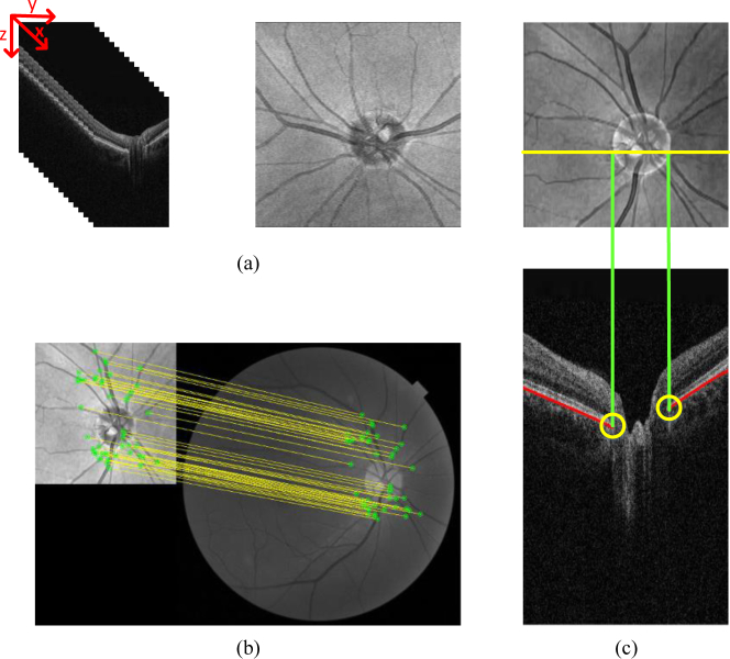
Considering the difficulty of BMO detection in an entire OCT slice, a coarse detection to determine the ROI is needed. Fig. 2 indicates that the coarse detection contains two steps: optic disc segmentation and RPE layer segmentation.

Fig. 2.

Coarse detection. (a) Original SD-OCT images and 2D projection images. (b) Registration between the projection and fundus images. (c) Diagram of the coarse detection, intersection (yellow) (yellow) of the RPE layer (red), and projection line of the disc (green) are the coarse detection results.

Optic disc segmentation

As BMO is the true position of the optic disc, segmenting the disc can be a reasonable way to locate BMO. Segmentation of the optic disc in the 2D projection image has three steps. First, each B-scan is denoised by employing the block-matching 3D (BM3D) algorithm [23], and 3D SD-OCT volumes are resampled to create 2D projection images, the 2D projection image is created by averaging the voxel intensities in the z-direction in the SD-OCT volumes, as shown in Fig. 2(a). Second, the optic disc in the color fundus image is segmented [24]. Third, a robust registration algorithm [25], which is shown in Fig. 2(b), is used to align the color fundus image and the projection image. In the registration algorithm, the features from accelerated segment test-partial intensity invariant feature descriptor framework are used to extract the interest points from the multi-modal images, and then a single Gaussian robust point matching model is applied to match the features and eliminate the outliers.

RPE layer segmentation

A conditional random field (CRF) based method [26] is utilized to segment the RPE layer. The method trains a structured support vector machine to construct the energy of the CRF to segment the layers, the coarse BMO is obtained according to the result of disc segmentation and RPE layer segmentation. Moreover, the RPE layer segmentation also used to deal with the B-scan that near the boundary of the segmented disc. In this case, we segment the RPE layer of five B-scans out of the topmost and bottom points of the coarse optic disc boundary and get the inflection point as the coarse BMO in order to contain as many images with BMO as possible.

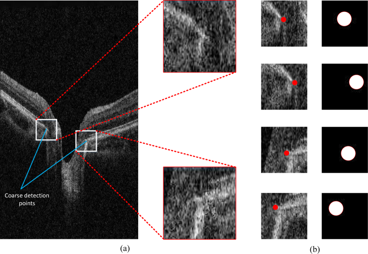
As shown in Fig. 2(c), the coarse detection result is the intersection of the RPE layer and the projection line of the optic disc. Once the results of coarse detection are obtained, the ROI is selected as an 80×80 patch centered on the coarse detection points, as shown in Fig. 3(a).

Fig. 3.

Data process.(a) ROI determination. (b) Label transformation for different patches.

2.2. Fixed detection based on U-net

Given the influence of optic disc segmentation and registration, the coarse detection results show relatively low accuracy and stability. In this section, we introduce a fixed detection stage based on the CNN to further improve the accuracy.

2.2.1. Data process for training

In the training stage, the two ROIs (one represents the left BMO and the other represents the right) in each OCT B-scan are selected according to the ground truth. We randomly obtain several 64×64 patches in each ROI region. To further enlarge the dataset, we utilize the augmentation containing random rotation and horizontal flips.

Considering the difficulty for the model to detect a single point in the patch, we extend the label to a circle region centered at BMO with a radius r and then transform the problem to the segmentation task of the circular region. As a result, the effect of imbalanced data is decreased and additional neighborhood information is learned to distinguish BMO and the border tissue. Fig. 3(b) shows the labels that are transformed into the circular region.

2.2.2. Network architecture and training details

The U-net [27] is efficient in the domain of medical image segmentation. Thus, the fixed detection stage in our proposed method is based on U-net, as shown in Fig. 4.

Fig. 4.

U-net architecture in our proposed method.

Considering the unavoidable noises and border tissues around BMO, we combine the denoised image generated by BM3D with the original image to compose a dual-channel image. Then, the dual-channel image is sent to U-net to produce improved detection results.To avoid over-fitting, we employ dropout and L2 normalization.

We use the Stochastic Gradient Descent optimizer with 0.9 momentum. The learning rate is set to 0.001 and is gradually decreased. The dropout rate is 0.5, and the λ of L2 normalization is 1e-5.

2.2.3. Loss function

Given the remaining problem of the imbalanced class, the loss function in our network is based on the dice loss. The dice coefficient is a general measure for segmentation, first proposed by Milletari et al. [28] as a loss function for the medical image analysis. The dice loss is formulated as Eq. (1):

$$DL=1-\frac{2{{\displaystyle \sum }}_x^{\Omega }{p}_x{g}_x}{{{\displaystyle \sum }}_x^{\Omega }{p}_x^2{{\displaystyle \sum }}_x^{\Omega }{g}_x^2}$$ (1)

where p_x and g_x represent the prediction result and ground truth with the pixel x in the patch Ω, respectively, ${\displaystyle \sum }_x^{\mathrm{\Omega }}{p}_x$ and ${\displaystyle \sum }_x^{\mathrm{\Omega }}{g}_x$ represent the number of pixels in prediction and ground truth region, so that ${\displaystyle \sum }_x^{\mathrm{\Omega }}{p}_x{g}_x$ indicates the true positive area of prediction compared to the ground truth.

As mentioned above, the circular region centered on the true BMO is marked as the ground truth. However, the area of the output is always too small to achieve a high dice coefficient. To solve this problem, we add an area bias in the dice loss, formulated as Eq. (2):

$$AL=1-\frac{min\left({{\displaystyle \sum }}_x^{\Omega }{p}_x,{{\displaystyle \sum }}_x^{\Omega }{g}_x\right)}{max\left({{\displaystyle \sum }}_x^{\Omega }{p}_x,{{\displaystyle \sum }}_x^{\Omega }{g}_x\right)}$$ (2)

To balance the accuracy of the output, we add the mean square error (MSE) loss because it is smoother than the cross-entropy. The final loss function of our proposed method is given by Eq. (3):

$$\begin{array}{ll}Loss\hfill & =DL+AL+MSE\hfill \\ \hfill & =2-\frac{2{{\displaystyle \sum }}_x^{\Omega }{p}_x{g}_x}{{{\displaystyle \sum }}_x^{\Omega }{p}_x^2{{\displaystyle \sum }}_x^{\Omega }{g}_x^2}-\frac{min\left({{\displaystyle \sum }}_x^{\Omega }{p}_x,{{\displaystyle \sum }}_x^{\Omega }{g}_x\right)}{max\left({{\displaystyle \sum }}_x^{\Omega }{p}_x,{{\displaystyle \sum }}_x^{\Omega }{g}_x\right)}+\frac{1}{n}{\displaystyle \sum }_x^{\mathrm{\Omega }}{(p_x-g_x)}^2\hfill \end{array}$$ (3)

where n is the summary of the pixels in the region Ω.

2.3. Post-processing

The border tissue caused by peripapillary atrophy is highly similar to BMO [29], as shown in Fig. 5 (a), which confuses the model to identify the BMO region centered on the border tissue instead of the end of the BM surface and causes some outliers. To remove the outliers caused by the border tissue, we propose a post-processing algorithm. Considering that most of the results of patches produced by the network are correct, we can utilize the correct results and eliminate the outliers. The ROI of the test image is cropped into several patches in an overlapping manner, and then several patches are sent to the trained network simultaneously. Finally, we choose the best result by the metrics defined in Eq. (4):

$$M_i={\displaystyle \sum }_{j=1,i\ne j}^{m}Dice{(S_i,S_j)}^k$$ (4)

where m is the patch of each test image. For adapting the size of ROI and patches, $S_i,S_j$ indicates the segmentation map of the i-th and j-th patches of the ROI image I, $Dice\left(S_i,S_j\right)=\frac{{{\displaystyle \sum }}_x^{\Omega }{S}_{ix}{S}_{jx}}{{{\displaystyle \sum }}_x^{\Omega }{S}_{ix}+{{\displaystyle \sum }}_x^{\Omega }{S}_{jx}}$ is the dice coefficient of the $S_i,S_j$, and k is an exponential parameter which is used to enlarge the consistent components and eliminate the effects of small dice value. At last, the center of the segmentation map is extracted as the final results of BMO detection, formulated as Eq. (5):

$$C=Center\left(S_d\right),d=\underset{i}{\text{arg max}}{M}_i,i=1,2\dots m$$ (5)

where d is the index of the patch that has a maximum M, $Center()$ represents the geometric center of the segmentation map, and C indicates the results of BMO points. The sketch map of post-processing is shown as Fig. 5(b).

Fig. 5.

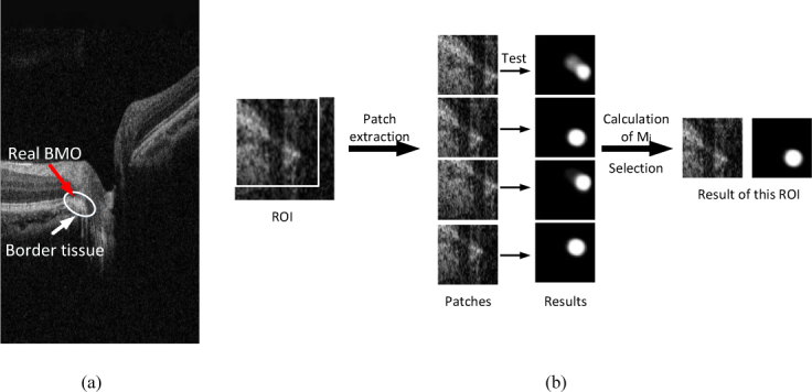
Illustration of the border tissue and the post-processing steps. (a) The sketch map of ambiguous border tissue. The real BMO is confused by the border tissue in this case. (b) The sketch map of post-processing. There are four patches (the box in the ROI indicate the upper left patch) extracted in the ROI and send to the trained U-net, the mask of patches with maximum Mi is selected as the result and its center point is the final result of BMO.

3. Results

3.1. Dataset

In this work, our proposed method is evaluated in 30 SD-OCT volumes, which are collected from the device Topcon 3D OCT-1 Maestro at the second Xiangya Hospital of Central South University. The size of each volume is 885×512×128 voxels, which represents 6 mm×6 mm×2 mm in the x-y-z direction. We use 80% and 20% of the dataset to train and test the U-net, respectively. The BMO points are marked by experts on all B-scans centered on the ONH region.

3.2. Experiments on method design

In this section, we describe a set of experiments to study the impact of different parameters, including radius parameters of the circular region, loss function components, and post-processing, on the performance of our proposed method as assessed by computing the accuracy of region segmentation and the mean error of BMO detection.

3.2.1. Effect of radius parameters of the circular region

The radius of the circular region indicates the neighborhood information sent to the U-net. For instance, the imbalanced class cannot be effectively solved if the radius is overly small, and unnecessary background could mislead the model if the radius is overly large.

In order to exclude the effects of area bias, we evaluated various radius parameters on the model with and without area bias. The results obtained with different radii are shown in Fig. 6. Regardless of the radius, the mean error becomes significantly larger than the properly radius, especially in the model results with loss function without area bias. We choose the radius = 9 in our experiment.

Fig. 6.

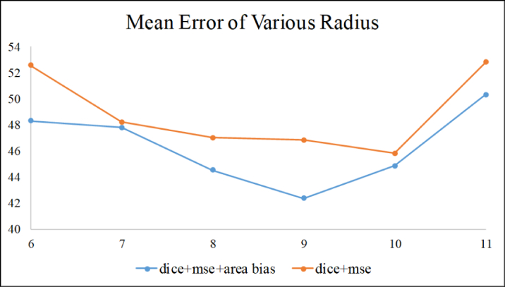
Results of various radius parameters.

3.2.2. Effect of loss function components

The effectiveness of our proposed loss function is evaluated through comparisons with simplified versions of our proposed loss function with only a subset of the three components mentioned above: 1) dice, 2) dice+MSE, 3) dice+area bias, and 4) dice+area bias+MSE.

As shown in Table 1, the combination of dice loss, MSE, and our proposed area bias outperforms the other subsets. Adding the proposed area bias to the loss function improves the result to 42.38 μm in the mean error, which indicates the benefit of the area bias. In addition, the MSE loss components further improve the performance by preventing the network from predicting two separate small regions caused by the vessel shadows.

Table 1.

Evaluation of the effect of loss function components

Components of loss function	Accuracy (%)	Mean error (μm)
Dice (group 1)	94.6	48.42
Dice+MSE (group 2)	95.2	46.84
Dice+area bias (group 3)	95.3	43.98
Dice+area bias+MSE (group 4)	95.9	42.38

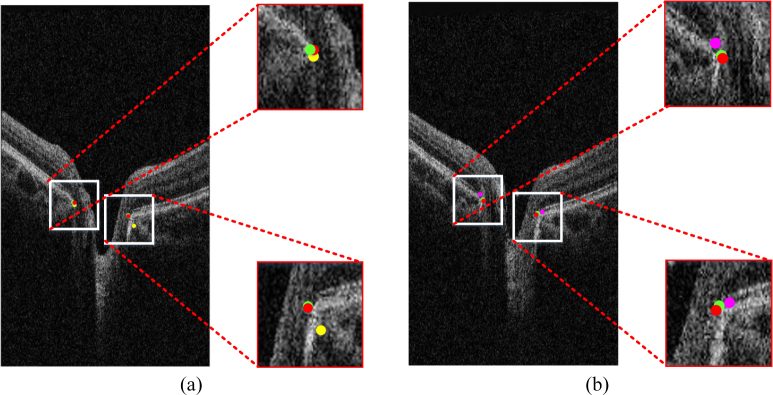
Fig. 7(a) shows the comparison of groups 2 and 4. The result of loss function without the area bias can be influenced by the border tissue, but group 4 avoids this problem and is highly consistent to the ground truth. Fig. 7(b) shows that the result accuracy decreases in the absence of MSE components.

Fig. 7.

Result of various loss function components. (a) Results of group 4 (green), group 2 (yellow), and the ground truth (red). (b) Results of group 4 (green), group 3 (pink), and the ground truth (red). Best viewed in color.

3.2.3. Effect of the post-processing

To evaluate our proposed post-processing algorithm, we compared the method without post-processing with our proposed method under several conditions. As shown in Table 2, the mean error of the method without post-processing is 5-7 μm larger than that of the method with post-processing, indicating that our proposed post-processing algorithm plays a significant role in our detection method. Furthermore, the result of the method without post-processing proves the benefits of area bias loss components.

Table 2.

Evaluation of the effect of post-processing

	Components of loss function	Mean error (μm)
Method with post-processing	Dice	48.42
	Dice+MSE	46.84
	Dice+area bias	43.98
	Dice+area bias+MSE	42.38
Method without post-processing	Dice	53.27
	Dice+MSE	52.30
	Dice+area bias	49.82
	Dice+area bias+MSE	49.29

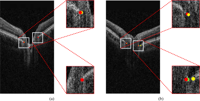
As shown in Fig. 8(a), the results of the method with and without post-processing and the ground truth are almost the same. However, the result of the method without post-processing can have a relatively large deviation, as shown in Fig. 8(b). This result indicates that our proposed post-processing algorithm can remove some outliers.

Fig. 8.

Evaluation of the effect of post-processing. The dots in red, green, and yellow represent the ground truth, the result with post-processing, and the result without post-processing, respectively. (a) Result of the method without post-processing is satisfactory. (b) Result of the method without post-processing has a large deviation. Best viewed in color.

3.3. BMO detection performance

To evaluate our proposed method, we compared our detection results with those obtained by the TBMR method proposed by Hussain et al. [17], the patch searching method proposed by Wu et al. [19], and the machine-learning graph-based method proposed by Miri et al. [20]. The mean error of the BMO detection was used as the metrics.

Table 3 shows the mean error of the methods mentioned above and our proposed method compared with the ground truth. Our proposed method obtains better results than the three previously proposed methods, and the results of standard deviation indicate that the stability of our proposed method is superior that TBMR method and the patch searching method, and close to the machine-learning graph-based method. The qualitative evaluation of our proposed method is shown in Fig. 9, and the BMO in the SD-OCT volume is detected and displayed in the 2D projection image. BMO is the true position of the optic disc, and the results are highly consistent with the ground truth.

Table 3.

Results of BMO detection

Methods	Mean error (μm)	Standard deviation (μm)
TBMR method [18]	54.18	53.74
patch searching method [19]	67.00	42.00
machine-learning graph-based method [20]	49.28	16.78
proposed method	42.38	18.33

Fig. 9.

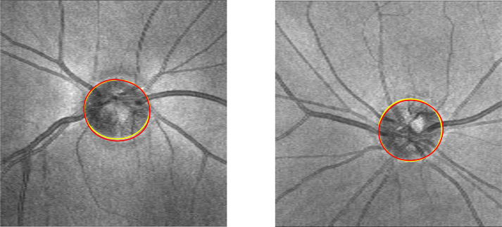
Comparison of our proposed method (yellow) with the ground truth (red) in the 2D projection image.

4. Discussion

To improve the precision of BMO detection and decrease the effect of border tissue and vessel shadows, we present a method for automatic BMO detection in SD-OCT volumes. Compared with other methods, our proposed method has several advantages. First, a three-stage detection framework is used. In the coarse detection, the RPE layer segmentation and the registration between the color fundus image and 2D projection image are employed. In the fixed detection, a U-net is utilized, and an area bias loss function is designed to achieve a high accuracy. Then, a post-processing algorithm is proposed to remove the outliers caused by the border tissue and further improve the performance. Second, instead of searching the entire SD-OCT B-scan, BMO is detected in the ROI determined by the stage of coarse detection. This strategy significantly improves the efficiency and accuracy of our proposed method. Third, the detection of a separate point is transformed to a region segmentation problem by marking the circular region centered on the BMO so that the problem of the imbalanced class is solved. Additional neighborhood information is sent to the model to guide the network learning to discriminate the BMO and the end of the border tissue.

Experimental results prove that the proposed method performs better than existing approaches and can thus be a clinical tool for BMO detection. However, this study also has some limitations. On the one hand, the influence of the vessel shadows and the border tissue caused by peripapillary atrophy cannot be completely eliminated. Thus, a robust compensation algorithm beyond the adaptive compensation [30] is needed to decrease the effects of vessel shadows and peripapillary atrophy. On the other hand, as the ROI is determined by the stage of coarse detection, our proposed method can only deal with the 3D SD-OCT volume because the coarse detection method of single B-scans is not robust enough. With a robust method to detect the ROI of BMO points in a single 2D OCT image, our proposed method can be applied to 2D OCT images by only replacing the coarse detection method.

It is worth noticing that the disc segmentation and registration in our coarse segmentation is not always satisfied enough. In this case, we also use the inflection point of the RPE layer as the coarse BMO points. Although the accuracy will decrease slightly, it will increase the stability of our proposed method. In future works, the ROIs could be extracted by region proposal network based method instead of the coarse detection.

5. Conclusion

In summary, we proposed a method for detecting the BMO points from SD-OCT volumes. The method contains a coarse detection stage, which is composed by an RPE layer segmentation and a multi-modal registration; a fixed detection stage based on the U-net; and a post-processing strategy to further improve the performance by decreasing the effects of the border tissue. Our proposed method enables accurate detection of BMO, leading to precise computation of the parameters based on the BMO points and accurate glaucoma diagnosis.

In future research, we plan to further improve our method in two ways. The network architecture will be modified to suit our detection goal, and a compensation method will be proposed to remove the vessel shadows and increase the contrast of the border tissue and RPE layer.

Funding

National Natural Science Foundation of China (61672542, 81670859); Fundamental Research Funds for the Central Universities of Central South University (2018zzts567).

Disclosures

The authors declare that there are no conflicts of interest related to this article.

References

- 1.Weinreb R. N., Khaw P. T., “Primary open-angle glaucoma,” The Lancet 363, 1711–1720 (2004). 10.1016/S0140-6736(04)16257-0 [DOI] [PubMed] [Google Scholar]
- 2.Yousefi S., Goldbaum M. H., Balasubramanian M., Jung T., Weinreb R. N., Medeiros F. A., Zangwill L. M., Liebmann J. M., Girkin C. A., Bowd C., “Glaucoma progression detection using structural retinal nerve fiber layer measurements and functional visual field points,” IEEE Transactions on Biomed. Eng. 61, 1143–1154 (2014). 10.1109/TBME.2013.2295605 [DOI] [PMC free article] [PubMed] [Google Scholar]
- 3.Mwanza J.-C., Chang R. T., Budenz D. L., Durbin M. K., Gendy M. G., Shi W., Feuer W. J., “Reproducibility of peripapillary retinal nerve fiber layer thickness and optic nerve head parameters measured with cirrus hd-oct in glaucomatous eyes,” Investig. Ophthalmol. & Vis. Sci. 51, 5724 (2010). 10.1167/iovs.10-5222 [DOI] [PMC free article] [PubMed] [Google Scholar]
- 4.Manassakorn A., Nouri-Mahdavi K., Caprioli J., “Comparison of retinal nerve fiber layer thickness and optic disk algorithms with optical coherence tomography to detect glaucoma,” Am. J. Ophthalmol. 141, 105 –115.el (2006). 10.1016/j.ajo.2005.08.023 [DOI] [PubMed] [Google Scholar]
- 5.Belghith A., Bowd C., Medeiros F. A., Hammel N., Yang Z., Weinreb R. N., Zangwill L. M., “Does the location of bruch’s membrane opening change over time? longitudinal analysis using san diego automated layer segmentation algorithm (salsa),” Investig. Ophthalmol. & Vis. Sci. 57, 675 (2016). 10.1167/iovs.15-17671 [DOI] [PMC free article] [PubMed] [Google Scholar]
- 6.Chauhan B. C., O’Leary N., AlMobarak F. A., Reis A. S., Yang H., Sharpe G. P., Hutchison D. M., Nicolela M. T., Burgoyne C. F., “Enhanced detection of open-angle glaucoma with an anatomically accurate optical coherence tomography–derived neuroretinal rim parameter,” Ophthalmology 120, 535–543 (2013). 10.1016/j.ophtha.2012.09.055 [DOI] [PMC free article] [PubMed] [Google Scholar]
- 7.Gmeiner J. M., Schrems W. A., Mardin C. Y., Laemmer R., Kruse F. E., Schrems-Hoesl L. M., “Comparison of bruch’s membrane opening minimum rim width and peripapillary retinal nerve fiber layer thickness in early glaucoma assessment,” Investig. Ophthalmology & visual science 57, OCT575 (2016). 10.1167/iovs.15-18906 [DOI] [PubMed] [Google Scholar]
- 8.Chen Z.-L., Peng P., Zou B.-J., Shen H.-L., Wei H., Zhao R.-C., “Automatic anterior lamina cribrosa surface depth measurement based on active contour and energy constraint,” J. Comput. Sci. Technol. 32, 1214–1221 (2017). 10.1007/s11390-017-1795-y [DOI] [Google Scholar]
- 9.Kim Y., Kim D., Jeoung J., Kim D., Park K., “Peripheral lamina cribrosa depth in primary open-angle glaucoma: a swept-source optical coherence tomography study of lamina cribrosa,” Eye 29, 1368 (2015). 10.1038/eye.2015.162 [DOI] [PMC free article] [PubMed] [Google Scholar]
- 10.Yin F., Liu J., Ong S. H., Sun Y., Wong D. W., Tan N. M., Cheung C., Baskaran M., Aung T., Wong T. Y., “Model-based optic nerve head segmentation on retinal fundus images,” in Engineering in Medicine and Biology Society, EMBC, 2011 Annual International Conference of the IEEE, (IEEE, 2011), pp. 2626–2629. [DOI] [PubMed] [Google Scholar]
- 11.Cheng J., Liu J., Xu Y., Yin F., Wong D. W. K., Tan N.-M., Tao D., Cheng C.-Y., Aung T., Wong T. Y., “Superpixel classification based optic disc and optic cup segmentation for glaucoma screening,” IEEE transactions on Medical Imaging 32, 1019–1032 (2013). 10.1109/TMI.2013.2247770 [DOI] [PubMed] [Google Scholar]
- 12.Zheng Y., Stambolian D., O’Brien J., Gee J. C., “Optic disc and cup segmentation from color fundus photograph using graph cut with priors,” in International Conference on Medical Image Computing and Computer-Assisted Intervention, (Springer, 2013), pp. 75–82. [DOI] [PMC free article] [PubMed] [Google Scholar]
- 13.Fu H., Cheng J., Xu Y., Wong D. W. K., Liu J., Cao X., “Joint optic disc and cup segmentation based on multi-label deep network and polar transformation,” arXiv preprint arXiv:1801.00926 (2018). [DOI] [PubMed]
- 14.Hu Z., Abramoff M. D., Kwon Y. H., Lee K., Garvin M. K., “Automated segmentation of neural canal opening and optic cup in 3d spectral optical coherence tomography volumes of the optic nerve head,” Investig. ophthalmology & visual science 51, 5708–5717 (2010). 10.1167/iovs.09-4838 [DOI] [PMC free article] [PubMed] [Google Scholar]
- 15.Miri M. S., Abràmoff M. D., Lee K., Niemeijer M., Wang J.-K., Kwon Y. H., Garvin M. K., “Multimodal segmentation of optic disc and cup from sd-oct and color fundus photographs using a machine-learning graph-based approach,” IEEE Transactions on Med. Imaging 34, 1854–1866 (2015). 10.1109/TMI.2015.2412881 [DOI] [PMC free article] [PubMed] [Google Scholar]
- 16.Fu H., Xu D., Lin S., Wong D. W. K., Liu J., “Automatic optic disc detection in oct slices via low-rank reconstruction,” IEEE Transactions on Biomed. Eng. 62, 1151–1158 (2015). 10.1109/TBME.2014.2375184 [DOI] [PubMed] [Google Scholar]
- 17.Belghith A., Bowd C., Weinreb R. N., Zangwill L. M., “A hierarchical framework for estimating neuroretinal rim area using 3d spectral domain optical coherence tomography (sd-oct) optic nerve head (onh) images of healthy and glaucoma eyes,” in Engineering in Medicine and Biology Society (EMBC), 2014 36th Annual International Conference of the IEEE, (IEEE, 2014), pp. 3869–3872. [DOI] [PubMed] [Google Scholar]
- 18.Hussain M. A., Bhuiyan A., Ramamohanarao K., “Disc segmentation and bmo-mrw measurement from sd-oct image using graph search and tracing of three bench mark reference layers of retina,” in Image Processing (ICIP), 2015 IEEE International Conference on, (IEEE, 2015), pp. 4087–4091. 10.1109/ICIP.2015.7351574 [DOI] [Google Scholar]
- 19.Wu M., Leng T., de Sisternes L., Rubin D. L., Chen Q., “Automated segmentation of optic disc in sd-oct images and cup-to-disc ratios quantification by patch searching-based neural canal opening detection,” Opt. Express 23, 31216–31229 (2015). 10.1364/OE.23.031216 [DOI] [PubMed] [Google Scholar]
- 20.Miri M. S., Abràmoff M. D., Kwon Y. H., Sonka M., Garvin M. K., “A machine-learning graph-based approach for 3d segmentation of bruch’s membrane opening from glaucomatous sd-oct volumes,” Med. Image Analysis 39, 206–217 (2017). 10.1016/j.media.2017.04.007 [DOI] [PMC free article] [PubMed] [Google Scholar]
- 21.Fang L., Cunefare D., Wang C., Guymer R. H., Li S., Farsiu S., “Automatic segmentation of nine retinal layer boundaries in oct images of non-exudative amd patients using deep learning and graph search,” Biomed. Opt. Express 8, 2732–2744 (2017). 10.1364/BOE.8.002732 [DOI] [PMC free article] [PubMed] [Google Scholar]
- 22.Venhuizen F. G., van Ginneken B., Liefers B., van Asten F., Schreur V., Fauser S., Hoyng C., Theelen T., Sánchez C. I., “Deep learning approach for the detection and quantification of intraretinal cystoid fluid in multivendor optical coherence tomography,” Biomed. Opt. Express 9, 1545–1569 (2018). 10.1364/BOE.9.001545 [DOI] [PMC free article] [PubMed] [Google Scholar]
- 23.Dabov K., Foi A., Katkovnik V., Egiazarian K., “Image denoising by sparse 3-d transform-domain collaborative filtering,” IEEE Transactions on image processing 16, 2080–2095 (2007). 10.1109/TIP.2007.901238 [DOI] [PubMed] [Google Scholar]
- 24.Lu S., “Accurate and efficient optic disc detection and segmentation by a circular transformation,” IEEE Transactions on medical imaging 30, 2126–2133 (2011). 10.1109/TMI.2011.2164261 [DOI] [PubMed] [Google Scholar]
- 25.Wang G., Wang Z., Chen Y., Zhao W., “Robust point matching method for multimodal retinal image registration,” Biomed. Signal Process. and Control. 19, 68–76 (2015). 10.1016/j.bspc.2015.03.004 [DOI] [Google Scholar]
- 26.Chakravarty A., Sivaswamy J., “A supervised joint multi-layer segmentation framework for retinal optical coherence tomography images using conditional random field,” Comput. Methods and Programs in Biomed. 165, 235–250 (2018). 10.1016/j.cmpb.2018.09.004 [DOI] [PubMed] [Google Scholar]
- 27.Ronneberger O., Fischer P., Brox T., “U-net: Convolutional networks for biomedical image segmentation,” in International Conference on Medical image computing and computer-assisted intervention, (Springer, 2015), pp. 234–241. [Google Scholar]
- 28.Milletari F., Navab N., Ahmadi S.-A., “V-net: Fully convolutional neural networks for volumetric medical image segmentation,” in 3D Vision (3DV), 2016 Fourth International Conference on, (IEEE, 2016), pp. 565–571. 10.1109/3DV.2016.79 [DOI] [Google Scholar]
- 29.Hwang Y. H., Jung J. J., Park Y. M., Kim Y. Y., Woo S., Lee J. H., “Effect of myopia and age on optic disc margin anatomy within the parapapillary atrophy area,” Jap. J. Ophthalmol. 57, 463–470 (2013). 10.1007/s10384-013-0263-7 [DOI] [PubMed] [Google Scholar]
- 30.Mari J. M., Strouthidis N. G., Park S. C., Girard M. J., “Enhancement of lamina cribrosa visibility in optical coherence tomography images using adaptive compensation,” Investig. ophthalmology & visual science 54, 2238–2247 (2013). 10.1167/iovs.12-11327 [DOI] [PubMed] [Google Scholar]