Abstract
Endoscopic optical coherence tomography (OCT) devices are capable of generating high-resolution images of esophageal structures at high speed. To make the obtained data easy to interpret and reveal the clinical significance, an automatic segmentation algorithm is needed. This work proposes a fast algorithm combining sparse Bayesian learning and graph search (termed as SBGS) to automatically identify six layer boundaries on esophageal OCT images. The SBGS first extracts features, including multi-scale gradients, averages and Gabor wavelet coefficients, to train the sparse Bayesian classifier, which is used to generate probability maps indicating boundary positions. Given these probability maps, the graph search method is employed to create the final continuous smooth boundaries. The segmentation performance of the proposed SBGS algorithm was verified by esophageal OCT images from healthy guinea pigs and the eosinophilic esophagitis (EoE) models. Experiments confirmed that the SBGS method is able to implement robust esophageal segmentation for all the tested cases. In addition, benefiting from the sparse model of SBGS, the segmentation efficiency is significantly improved compared to other widely used techniques.
1. Introduction
Optical coherence tomography (OCT) as a powerful medical imaging technique can generate high-resolution cross-section images of biological tissues non-invasively [1]. Initial applications of OCT were mainly in ophthalmology and have achieved numerous success in retinal disease diagnosis [2–4]. By combining fiber-optic flexible endoscopes, OCT is able to enter the upper gastrointestinal tract [5, 6]. In that case, it can image the microscopic structure of the esophagus, which helps to diagnose a variety of esophageal diseases, such as Barrett’s esophagus (BE) [7, 8], eosinophilic esophagitis (EoE) [9], and dysplasia [10]. Esophageal diseases are identified from OCT images by observing abnormalities in tissue microstructures, such as changes in layer thickness or disruption to the layers. For instance, BE has an irregular mucosal surface and may present an absence of the layered architecture [7]; EoE is often featured with increased basal zone thickness [9]. Finding these diseased characteristics by observing or manual segmentation is time-consuming and requires specific domain knowledge. As a result, a computer-aided layer segmentation method is urgently needed, as employed in ophthalmology [11, 12].
Representative segmentation techniques for OCT images can be grouped into two main categories. The first group is based on mathematical models. Methods of this kind build a mathematical model based on apriori assumptions of the input image structure and locate boundaries by optimizing the model. Typical methods in this class include the A-scan based methods [2, 3, 13], the active contour [4, 14–17] and graph based methods [18–22]. The second category is machine learning based methods. Such methods formulate the segmentation into a classification problem. Features reflecting layer structure characteristics are extracted for the training, and boundaries of new images are located by pixel classifying using the trained model. Following this process, Vermeer et al. used the Haar-like features and the Support Vector Machine (SVM) to implement retinal segmentation [23]. Lang et al. employed the random forest (RF) classifier and 27 features that provide spatial, local and context awareness to segment eight retinal layers [24]. Recently, the newly developed deep learning technique, especially convolutional neural networks attracts wide attentions in the field of medical image analysis and has achieved great success in OCT image segmentation [25–28]. Different from traditional machine learning techniques, deep learning is able to learn optimal features directly from the training data and achieves higher classification accuracy [29]. However, deep learning based segmentation relies on a large number of annotated data and suffers from high computational burdens [25].
Most existing reports on esophageal OCT image segmentation employed the model-based approach. For example, Ughi used an A-scan based method to locate the esophageal wall position [30]. Zhang et al. used the graph theory dynamic program (GTDP) to implement five-layer segmentation [31]. On this basis, Gan et al. combined modified Canny edge detection with GTDP to realize more accurate segmentation [32]. To the best of our knowledge, the GTDP is the first effective framework to segment five esophageal layers [31]. However, some problems limit its application. Firstly, GTDP requires tissues to have similar widths in the same layer across the image, otherwise it will generate a fairly biased output. In other words, GTDP is difficult to deal with the possible variations in esophageal tissues. Secondly, it takes about 6 to10 seconds to segment a single B-scan [31, 32], which is less efficient.
To solve these problems, this study proposes a sparse Bayesian graph search (SBGS) method that combines sparse Bayesian classification [33, 34] and the GTDP for esophageal layer segmentation. Sparse Bayesian classification is a Bayesian extension of SVM [35] that trains classifiers under a series of probability assumptions. It uses a prediction model similar to SVM, but with much less “support vectors” resulting from a sparsity assumption, thus ensuring high classification efficiency. Sparsity assumption is widely adopted in signal and image processing and has been confirmed to be effective in OCT image analysis as discussed in the literature [36, 37]. Another advantage of the sparse Bayesian classifier is that the probability output can be further optimized to generate the final boundary. The proposed SBGS algorithm consists of the following steps. Firstly, representative features were extracted to delineate esophageal layer structures. In detail, this study utilizes the multi-scale gradients and averages [38] to describe intensity changes along A-scan at different scales. Besides, the Gabor wavelet features [39] are also employed as a supplementary description of boundary information in other directions. Given these features, a sparse Bayesian classifier is trained to estimate the position of esophageal layer boundaries and generate a probability map. Finally, a graph is constructed based on the probability map, which is further optimized by the GTDP to get continuous smooth boundaries that segment different tissue layers. Benefitting from sparse Bayesian classification and the GTDP, the proposed SBGS method is able to achieve fast esophageal layer segmentation and will be robust in segmenting OCT images with irregular tissue layers.
In summary, our main contribution is implementing a fast segmentation of esophageal OCT images obtained from guinea pigs. More detailedly, this work contributes to extract features that comprehensively describe esophageal tissue layers based on wavelet-related theories. Besides, an efficient boundary identification scheme was designed using sparse Bayesian representation. Finally, segmentation experiments on esophageal OCT images from guinea pigs were performed to evaluate the generalization ability and clinical potential of proposed SBGS algorithm.
The rest of this study is organized as follows. Section 2 describes the details of the proposed SBGS algorithm for esophageal layer segmentation. Section 3 presents experimental results on esophageal OCT images from guinea pigs. Discussions and conclusions are given in Sections 4 and 5, respectively.
2. Methods
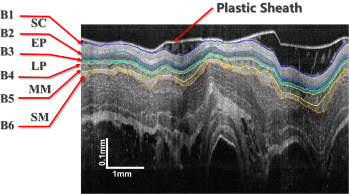
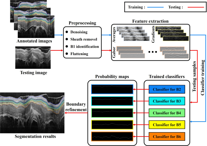
The performance of our method is evaluated by segmenting endoscopic OCT images of guinea pig esophagus. A typical OCT image is shown in Fig. 1. The tissue layers marked in the images are the epithelium stratum corneum (SC), epithelium (EP), lamina propria (LP), muscularis mucosae (MM) and submucosa (SM), which are defined by boundaries to . Our SBGS algorithm intends to locate to fast and robustly, thus accomplishing proper segmentation of different tissue layers. The entire process is summarized in Fig. 2. Note that the algorithm is composed of four units. The preprocessing unit regularizes the data to make it appropriate for boundary identification. The second unit extracts features reflecting tissue structures. Given these features, a sparse Bayesian classifier is achieved by the classifier training unit, which can generate a probability map for the B-scan. Finally, the probability map is processed by the boundary refinement unit to obtain smooth continuous boundaries. Details implementation about these units are presented as follows.
Fig. 1.
A manual segmented esophageal OCT image from the guinea pig.
Fig. 2.
Flowchart of the SBGS algorithm.
2.1. Preprocessing
Several preprocessing steps were taken to make the data appropriate for classifier training, including denoising, plastic sheath removal and flattening. Image denoising is achieved with a simple median filter of size 7 × 7 considering its high efficiency and easy implementation. The effectiveness of it in OCT images denoising has been confirmed by several researches [3, 25, 40]. The sheath removal and flattening process is specifically designed for esophageal OCT images and is described below.
2.1.1. Plastic sheath removal
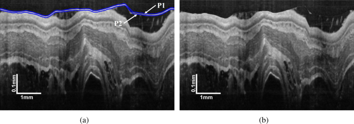
The plastic sheath is used to protect the probe from biofluid during the imaging process and is recorded on OCT images as shown in Fig. 1. Its boundary is so prominent that it causes strong disturbance for the detection of the esophageal lumen boundary. Therefore, it is necessary to remove such sheath and this study achieved this using the GTDP algorithm [20].
As shown in Fig. 3(a), the plastic sheath boundary often possesses the highest intensity contrast, which indicates owns the highest gradient that can be easily located by GTDP. On the basis of , can be detected by limiting the GTDP region to ten pixels below , which is an approximate sheath thickness. In that case, the plastic sheath can be removed by shifting the pixels from to and the empty pixels are filled with a mirror image. A typical result is shown in Fig. 3(b). Although there are some white regions between the plastic sheath and lumen boundary, these regions are not so prominent as the plastic sheath. As a result, the lumen boundary owns the highest gradient in this case, thus making it easily detected by the GTDP.
Fig. 3.
Plastic sheath removal: (a) position of and ; (b) image with the plastic sheath removed.
2.1.2. Lumen boundary detection and flattening
Subsequent preprocessing is to detect the esophageal lumen boundary ( in Fig. 1) and flatten the image based on it. This serves to provide spatial alignment of OCT images, which can help constrain the search area as well as reducing the algorithm sensitivity to tissue curvature.
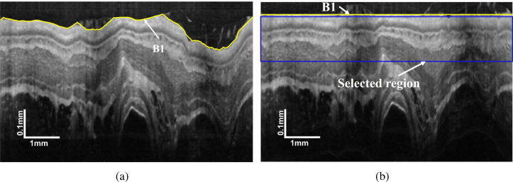
Lumen boundary detection is convenient using the GTDP because it is the most prominent layer boundary on an image without the plastic sheath (3(b)). As a result, it can be detected by the same process as identification. The lumen boundary is then flattened by translating the A-scans up and down. In that case, OCT images are regularized for the following segmentation as shown in Fig. 4. To reduce the memory size and improve the algorithm efficiency, the layer search area is constrained to the tissue-related regions. The total thickness of the five tissue layers for the guinea pig is 110 μm (125 pixels) in healthy condition and 150 μm (170 pixels) for the EoE model [31, 32]. Considering irregularities, limiting the search region from 5 pixels to 195 pixels below the lumen boundary (Fig. 4(b)) is sufficient for analyzing all those tissue layers.
Fig. 4.
Demonstration of (a) position of and (b) the flattened OCT image with marked selected region.
2.2. Feature extraction
An interface occurs as the OCT signal increases or decreases, resulting in intensity changes of pixels above and below the boundary. On this basis, two kinds of features were used in this study. Features of the first type are the multi-scale gradients and averages [38], which can reflect boundary information at different resolutions. Features of the second type are the Gabor wavelet coefficients, which provides boundary information in different orientations.
2.2.1. Multi-scale gradients and averages
Since the esophageal images have been flattened, gradients and averages along A-scan are more useful for layer boundary deteciton. Let denote the intensity alone A-scan, the averages hd at scale d are defined by
| (1) |
Accordingly, the gradients gd at scale d can be calculated by
| (2) |
Specifically, , . Multi-scale gradient and average features for pixel y can be summaried as
| (3) |
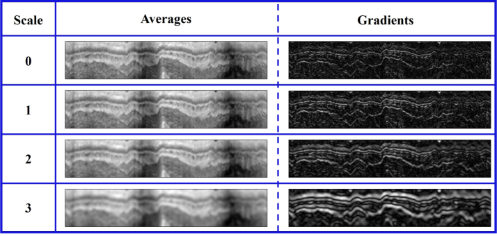
In this study, d is set at 4, indicating 8 features will be achieved. Typical gradient and average maps in different scales are shown in Fig. 5. It can be found that a lower scale feature map provides more precise description of local edges, whereas a higher scale feature map is more robust to noise and local distortion.
Fig. 5.
Demonstration of intensity averages and gradients at different scales.
2.2.2. Gabor wavelet features
Multiscale gradients only describe intensity changes along the A-scan. To provide information for layer boundaries in different directions, the Gabor wavelet features with directional selectivity were employed in this study.
The 2-D wavelet transform of an image I is defined as:
| (4) |
where ψθ is the 2-D mother wavelet, a denotes the scaling parameters, x0 and y0 represents the spatial shifting, and θ is the orientation parameter. The Gabor function can be used as the mother wavelet, which is defined by Eq. (5) [39],
| (5) |
where f is the frequency of the sinusoid, θ is the orientation of the major axis of the Gaussian, ϕ is the phase offset, σ is the standard deviation of the Gaussian and γ is a ratio parameter. The detailed implementation of the Gabor wavelets can be found in [39].
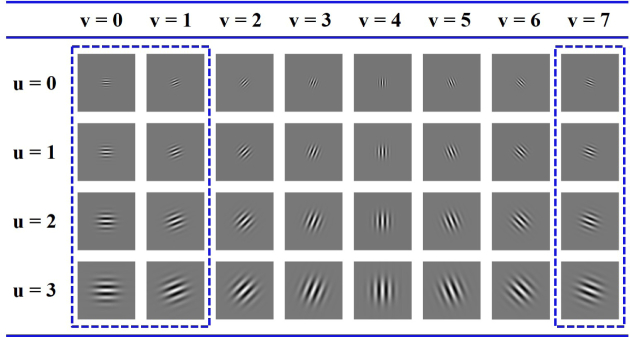
In this study, a family of Gabor wavelets is required to perform the multi-resolution analysis, which is defined as
| (6) |
where fu and θv defines the orientation and scale of the Gabor wavelets, is the maximum central frequency.
An example of Gabor wavelet coefficients at 4 scales and 8 orientations can be found in Fig. 6 with , , γ = 1. Considering the fact that the data were previously flattened, the wavelets with are sufficient for describing the layer boundaries as marked in Fig. 6. As a result, 12 Gabor features for each pixel will be obtained. Demonstration of Gabor wavelet features at different scales and orientations can be found in Fig. 7.
Fig. 6.
Demonstration of the Gabor wavelet coefficients.
Fig. 7.
Demonstration of Gabor wavelet features for esophageal OCT images.
Following the process above, we achieved 8 multi-scale gradient and average features and 12 Gabor wavelet features, totally 20 features for the subsequent boundary classification.
2.3. Sparse Bayesian classification
Suppose the data is denoted by , where xn is the feature vector, is the label for binary classification. Sparse Bayesian learning models the data based on the Bernoulli distribution, which indicates the likelihood can be expressed as
| (7) |
where is the sigmoid function, can be calculated by
| (8) |
is the kernel function, and the Gaussian Kernel is employed in this study as shown in Eq. (9).
| (9) |
To make the weight vector sparse, a zero-mean Gaussian prior distribution is set over w:
| (10) |
Following the assumptions described by Eqs. (7) to (10), an optimal can be obtained using the Laplace’s method [41]. For a new sample , the probability for can be calculated by
| (11) |
where xi indicates the relevance vector, which has nonzero wi, Nr is the relevance vector number. Since w is sparse, only a few xi are needed for a new sample identification, thus making the sparse Bayesian classification quite efficient.
The sparse Bayesian classifier using the Bernoulli model is a binary classifier, which can be generalized to deal with multi-class problems by the “one-versus-all” strategy [42] or öne-versus-one" strategy [42]. The main purpose of this study is to decide if a pixel belongs to any of the five boundaries. In this case, the “one-versus-all” strategy is more appropriate, separating the pixels on one boundary from the rest. Using this strategy, we trained five binary sparse Bayesian classifiers to detect pixels on boundaries to , respectively as shown in Fig. 2. To achieve the classifier for , points on the i-th boundary are treated as the positive samples (labeled "1"), and the remainders in the training set are regared as the negative samples (labeled "0"). In this way, we can model the data by Eq. (7) and achieve a binary sparse Bayesian classifier for boundary .
It is worth mentioning that the sparse Bayesian classifier can achieve multi-classification by modeling the data with multinomial distribution [33], but it suffers from a highly disadvantageous consequence from a computational perspective [33].
2.4. Boundary identification based on the classification result
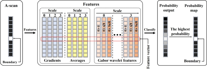
We marked the pixel with the highest probability in each A-scan to get the most likely boundary position. The boundary identification process can be depicted by Fig. 8. Note that each pixel was represented by a feature vector, which is then individually classified to achieve the final probability map. A typical result was shown in Fig. 9. Although the boundaries can be visually identified, there are still some missing parts or dropouts. As a result, the probability map needs to be further refined.
Fig. 8.
Flowchart of the boundary identification process.
Fig. 9.
Presentation of the boundary position indicated by sparse Bayesian classification. The probability map has a border painted with the same color as the corresponding boundary shown by the image on top left.
An intuitive way is to smooth the boundaries shown in Fig. 9 and inpaint the missing points. This method is simple and fast, but requires the classifier to be accurate and is susceptible to noise or other disturbance. A more robust approach is using the GTDP as in the references [24, 25]. This approach constructs a graph based on the probability map rather than the gradients and finds the optimal path by Dijkstra’s shortest path algorithm [20]. To refine the probability map for boundary , , the weight for edge connecting adjacent pixels a and b is defined as
| (12) |
where and are probability map intensities of for points a and b. is the minimum possible weight in the graph. More details about GTDP can be found in Chiu’s work [20]. It is worth mentioning that the search region for each boundary is pixels around the most probable boundary position, which will make the optimization more efficient. The region width is set based on the fact that the smallest tissue layer has a thickness of around 10 μm (11 pixels) [31, 32]. In that case, searching a certain boundary in pixels around the most probable position utilizes as much information as possible without inducing inference from boundaries of other tissue layers.
3. Experiments
3.1. Data and experimental environment
Esophageal OCT images from guinea pigs were obtained using an 800-nm ultrahigh resolution endoscopic OCT system [6, 43, 44]. Data from 4 subjects, including two healthy guinea pigs and two EoE models [45] were used to evaluate the proposed SBGS algorithm. For each subject, two datasets were obtained by the OCT system from different (deep and shallow) positions of the esophagus. Each dataset has 30 continuous imaged B-scans of size 2048 × 2048. More details about the data are listed in Table 1. The data was manually annotated by an experienced grader using ITK-SNAP [46]. Manual segmentation results were used for classifier training and algorithm evaluation. In the following experiments, the B-scans were resized by 0.5, which indicates the new size of B-scans is 1024 × 1024. Our images were analyzed by MATLAB on a personal computer with an Intel Core i7 2.20 GHz CPU and 16 GB RAM.
Table 1.
Information of the dataset used in this study.
| Datasets | Subject 1
|
Subject 2
|
Subject 3
|
Subject 4
|
||||
|---|---|---|---|---|---|---|---|---|
| Case 1 | Case 2 | Case 3 | Case 4 | Case 5 | Case 6 | Case 7 | Case 8 | |
| Condition | Healthy | Healthy | Healthy | Healthy | EoE | EoE | EoE | EoE |
| Position | Deep | Shallow | Deep | Shallow | Deep | Shallow | Deep | Shallow |
| Frames | 30 | 30 | 30 | 30 | 30 | 30 | 30 | 30 |
In the first part of the experiment, we performed the segmentation on each case separately, and took Case 1 as a representative example to numerically evaluated the SBGS algorithm in accuracy and efficiency. Since OCT images are collected continuously and consecutive frames have similar structure, we selected two well-imaged B-scans that roughly trisect Case 1 for training to ensure that our system does not become biased. The remaining 28 B-scans were used for testing. To show the generation and clinical potential of the proposed method, another experiment is performed using different training and testing sets. The training sets are composed of the four cases obtained from Subjects 1 and 3, each with 2 selected B-scans. The testing sets are composed of all the frames in Subjects 2 and 4. In this case, there was no overlap between subjects used for training and testing.
3.2. Accuracy analysis of the SBGS algorithm using Case 1
As is discussed above, the training and testing sets contain two B-scans and 28 B-scans respectively in this case. For a given B-scan of size 1024 × 1024, we used all the pixels on the boundaries (5 boundaries × 1024 points per boundary) for training. Since the number of non-boundary pixels is much larger than the boundary pixels, we randomly select 2048 non-boundary pixels to balance the training data.
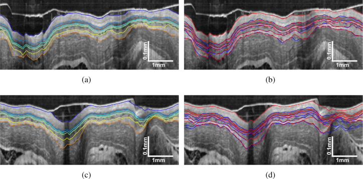
Using the trained sparse Bayesian classifier, the segmentation performance of SBGS can be evaluated by the test data. We first made an intuitive comparison between SBGS and the widely used GTDP algorithm as shown in Fig. 10. Figures 10(a) and 10(c) illustrate the SBGS segmentation results for OCT image with regular and irregular tissues, respectively. It can be found that the SBGS accomplished satisfactory segmentation in both cases. Specifically, we plotted the boundaries obtained by GTDP and SBGS in blue and red, respectively. In Fig. 10(b) with regular tissues, it can be vissually identified that the red lines generated by SBGS match the layer structures better. In Fig. 10(d) with larger thickness variations, the blue lines identified by GTDP show a great bias from the correct tissue structure while the SBGS can still identify the correct boundaries.
Fig. 10.
Demonstration of (a) SBGS segmentation result for OCT image with regular tissues; (b) comparisons of SBGS (red line) and GTDP (blue line) results; (c) SBGS segmentation result for OCT images with tissue irregularities and (d) comparisons of SBGS(red line) and GTDP (blue line) results.
To further evaluate the segmentation accuracy of the SBGS, we replaced the sparse Bayesian classifier with other classifiers widely used in OCT segmentation, including the SVM [23] and RF [24], thus achieving the SVM-GS and RF-GS methods. Parameters for different classifiers were set as follows. The sparse Bayesian learning and SVM utilized the Gaussian kernel described by Eq. (9) with . For SVM, the C-Support Vector Classification was employed [47] and the regularization parameter C is set at 4000 to achieve fewer support vectors. The main parameter for RF is the number of trees, which is set at 500 in this study.
The quantative evaluation was carried out by comparing the segmentation result of SBGS with SVM-GS, RF-GS and GTDP [20] using the manual segmentation as a reference. The unsigned border position differences between the automatic and manual segmentation for the 28 testing images from Case 1 are listed in Table 2. Results are presented in the form of mean ± standard deviation in micrometer, with bold data indicating the result with the smallest average difference. as the baseline for flattening was identified by the GTDP in all algorithms, hence the error values are almost identical. Except for , classifier-based methods (SBGS, SVM-GS, RF-GS) achieved more accurate boundary identification than the GTDP since they synthesized more comprehensive features to delineate the tissue structure. Besides, SBGS shows higher accuracy than SVM-GS because it uses fewer vectors to prevent overfitting and does not require optimization of the additional parameter C [47]. The segmentation result of RF-GS is comparable to SBGS in accuracy. In detail, SBGS achieved the most accurate segmentation in , and , while the RF-GS has higher accuracy in segmenting and .
Table 2.
Unsigned border position differences of different esophageal OCT image segmentation algorithms.
| Boundaries | SBGS | SVM-GS | RF-GS | GTDP |
|---|---|---|---|---|
| () | ||||
| () | ||||
| () | ||||
| () | ||||
| () | ||||
| () |
3.3. Efficiency analysis of the SBGS algorithm using Case 1
To evaluate the efficiency of the proposed algorithm, we listed the average segmentation time of SBGS, SVM-GS, RF-GS and GTDP in Table 3 for the testing data from Case 1. It is noted that the SBGS method is significantly faster than the other classifier-based methods. The main reason is that the sparse Bayesian classifier has a linear prediction model [Eq. (8)] that depends on much fewer relevance vectors as shown in Table 4. As a result, the classification can be implemented by a few linear operations, which is quite efficient. Moreover, the graph search is performed within a small region as illustrated in Section 2, thus making SBGS is also faster than GTDP.
Table 3.
Computation time for OCT image segmentation.
| Methods | SBGS | SVM-GS | RF-GS | GS |
|---|---|---|---|---|
| Time (s) |
Table 4.
Comparisons of Nr and the classification time for SVM and sparse Bayesian classifier (denoted by SBC).
| Boundaries |
Nr
|
Times (s)
|
||
|---|---|---|---|---|
| SVM | SBC | SVM | SBC | |
| B2 | 834 | 30 | ||
| B3 | 612 | 32 | ||
| B4 | 677 | 38 | ||
| B5 | 1043 | 39 | ||
| B6 | 895 | 31 | ||
For an intuitive explanation of why a sparse model is beneficial for efficient segmentation, we analyzed the detailed classification process of the sparse Bayesian classifier and the SVM. The classification of a new input for SVM depends on the support vectors (SVs), and the sparse Bayesian classifier has similar vectors, which are called relevance vectors (RVs) as shown in Eq. (11). Accordingly, the prediction efficiency is determined by the vector numbers for these two classifiers. In our segmentation framework, a B-scan generates pixels for training, each with 20 features. The classifier is trained using 2 representative B-scans, resulting in a training set of size 14336 × 20. The detailed analysis about the SVM and sparse Bayesian classifiers can be found in Table 4, where Nr represents the number of SVs and RVs used for classification. The sparse Bayesian classification achieved much smaller Nr than SVM, which indicates the boundary identification can be accomplished based on only a few tens of samples. As a result, the computation time can be remarkably reduced from around 1.5 to 0.15 seconds for recognizing a single boundary.
3.4. Generalization ability and clinical potential
To show the generalization ability and clinical potential of the SBGS algorithm, the training process is performed using images from a healthy guinea pig (Subject 1) and an EoE model (Subject 3), while the testing set is composed of Subjects 2 and 4. Detailedly, we selected two B-scans from each case in Subjects 1 and 3 using the same method as described in Section 3.1 to create the training set with eight B-scans. All of the frames obtained from Subjects 2 and 4 are used for testing, making the testing set of size frames.
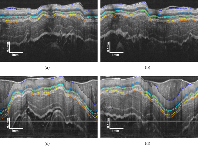
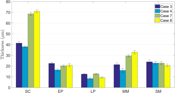
Representative segmentation results for the four testing cases can be found in Fig. 11. The tissue layers are well delineated for all the cases, which confirm that the SBGS algorithm is effective even if the layer structure changes due to such pathology. In addition, in this case, the training and testing sets are composed of images from different subjects, which indicates there is no overlap between training and testing, thus verifying the generalization ability of our method. Since EoE is often featured with increased basal zone thickness [9], we calculated the layer thicknesses based on the segmentation results. The corresponding statistic plot for layer thickness is presented in Fig. 12. Obviously, the SC layer thickness for EoE model is significantly larger than the normal one, thereby proving that the SBGS algorithm would potentially aid clinical diagnosis.
Fig. 11.
Representative segmentation result by SBGS of (a) Case 3 and (b) Case 4 from the testing healthy guinea pig (Subject 2); (c) Case 7 and (d) Case 8 from the testing EoE model (Subject 4).
Fig. 12.
Statistical results of layer thicknesses from different guinea pigs.
4. Discussions
This study used the sparse Bayesian classification for rapid esophageal layer segmentation in OCT images. The sparse Bayesian classifier offers some quite compelling and beneficial features. Firstly, the trained model is highly sparse, indicating that the prediction can be made based on a small number of samples, thus guaranteeing high classification efficiency. Besides, the noise variance can be automatically estimated. As a result, regularization parameters are no longer needed, such as C in SVM. Moreover, sparse Bayesian classification can provide a posterior probability of the sample, which is important for the following analysis, as discussed in Section 2.
The primary disadvantage of the sparse Bayesian method is the computational complexity of the training process [33]. The update rules required memory and computation scale respectively with the square and cube of the number of basis functions. In that case, sparse Bayesian learning may be less practical if the training sample number is large. Fortunately, since we only need the boundary pixels and a few background pixels for training, the model can be successfully learned. Sparse Bayesian classification needs longer training time compared to SVM and RF. In this study, sparse Bayesian classification takes about 10 minutes for model training with two B-scans, while SVM and RF only need 2 minutes and 1 minute, respectively.
Using the proposed algorithm, segmenting a single B-scan takes about 1.7 seconds with Matlab. The algorithm can be sped up by further optimizations. For example, a faster programming language, such as C can be employed. Besides, the classification of each pixel can be parallelly processed by multiple computer cores or the graphics processing unit (GPU). In that case, a more efficient segmentation system can be built, which can meet the requirements of online segmentation.
Experiments have proved that the SBGS algorithm is able to delineate EoE OCT data, suggesting that it has the potential to be extended for other esophageal diseases. Taking BE as an example, the OCT image of BE may present an absence of layered architecture. In that case, the SBGS is expected to implement tissue layer segmentation by extracting different features or adding a new criterion to locate regions with missing layers. Benefiting from the learning ability of sparse Bayesian classification, the SBGS will detect the pathological changes of the OCT image based on the annotated data, thus achieving automatical disease diagnosis.
It is worth mentioning that the deep learning based methods are very popular in image analysis, and has been introduced to retinal OCT image processing [25–28] recently. However, for esophageal OCT images discussed in this study, the deep network is hard to train due to the limited annotated samples. To verify this, we performed an additional experiment based on a representative deep learning based segmentation method proposed by Fang et al. [25] using the same training and testing sets as Section 3.2. The main idea is using a convolutional neural network (CNN) to extract features of specific layer boundaries and classifying the six layer boundaries on esophageal OCT image. According to Fang’s work [25], we extracted patches of size 33 × 33 pixels centered on each pixel of six annotated boundaries from OCT B-scans and marked them with labels 1-6. Besides, one randomly selected patch centered at the background for each A-scan is labeled with 0. In this case, the two B-scans in training set generated 14336 patches. The CNN architecture used in this experiment was summarized in Table 5.
Table 5.
The CNN architecture used in this experiment.
| Layers | Type | Filter Size | Neuron Numbers | Output Shape |
|---|---|---|---|---|
| Layer 1 | Convolution | 3 × 3 | 32 | |
| Layer 2 | Convolution | 3 × 3 | 64 | |
| Layer 3 | Max pool | – | – | |
| Layer 4 | Dropout | – | – | |
| Layer 5 | Flatten | – | – | 12544 × 1 |
| Layer 6 | Dense | – | 128 | 128 × 1 |
| Layer 7 | Dropout | – | – | 128 × 1 |
| Layer 8 | Dense | – | 7 | 7 × 1 |
It can be calculated that the number of parameters for this network is 1,625,479, which is difficult to optimize using the 14,336 patches. In this case, after 12 epochs optimization with batch size 128, the training accuracy is 0.7726 that cannot generate useful probability maps for boundary identification. When we add the training B-scans from 2 (14,336 patches) to 12 (86,016 patches), the training accuracy reached 0.9446 with the same configuration. It can be found that the CNN needs more annotated samples to optimize the huge number of parameters, which is in coincident with the discussion in [25]. In contrast, the SBGS algorithm showed effectiveness even if the train image is limited as discussed in Section 3.2.
5. Conclusions
In this study, we presented an SBGS method that combines sparse Bayesian learning and graph search for fast segmentation of layer boundaries on esophageal OCT images. The SBGS algorithm utilizes sparse Bayesian learning to build a classifier based on multi-scale gradients, averages and Gabor wavelet coefficients and generates a probability map of boundary positions. A graph is then constructed using the probability map, which is subsequently used to generate a continuous and smooth boundary by the graph search technique. In that case, esophageal layers are clearly segmented, making the OCT image easy to interpret. Experiments on segmenting OCT images from guinea pig esophagus demonstrated that the proposed SBGS method is robust and much faster than SVM-GS, RF-GS and the GTDP. In addition, segmentation experiments on esophageal OCT images from normal guinea pigs and EoE models confirmed that the SBGS algorithm has the potential to diagnose esophageal diseases. It is also appealing to apply the SBGS to other layered structure endoscopic OCT images (like airway) and non-endoscopic OCT images (like retina) in future work.
Acknowledgments
We would like to acknowledge Prof. Xingde Li and Dr. Wu Yuan from the Johns Hopkins University for their technical support in the SD-OCT systems and animal experiments.
Funding
National Key R&D Program for Major International Joint Research of China (2016YFE0107700). Jiangsu Planned Projects for Postdoctoral Research Funds of China (2018K007A, 2018K044C).
Disclosures
The authors declare that there are no conflicts of interest related to this article.
References
- 1.Huang D., Swanson E. A., Lin C. P., Schuman J. S., Stinson W. G., Chang W., Hee M. R., Flotte T., Gregory K., Puliafito C. A., Fujimoto J. G., “Optical coherence tomography,” Science 254, 1178–1181 (1991). 10.1126/science.1957169 [DOI] [PMC free article] [PubMed] [Google Scholar]
- 2.Hee M. R., Izatt J. A., Swanson E. A., Huang D., Schuman J. S., Lin C. P., Puliafito C. A., Fujimoto J. G., “Optical coherence tomography of the human retina,” Arch. Ophthalmol. 113, 325–332 (1995). 10.1001/archopht.1995.01100030081025 [DOI] [PubMed] [Google Scholar]
- 3.Koozekanani D., Boyer K., Roberts C., “Retinal thickness measurements from optical coherence tomography using a markov boundary model,” IEEE Transactions on Med. Imaging 20, 900–916 (2001). 10.1109/42.952728 [DOI] [PubMed] [Google Scholar]
- 4.Fernandez D. C., Salinas H. M., Puliafito C. A., “Automated detection of retinal layer structures on optical coherence tomography images,” Opt. Express 13, 10200–10216 (2005). 10.1364/OPEX.13.010200 [DOI] [PubMed] [Google Scholar]
- 5.Tearney G. J., Brezinski M. E., Bouma B. E., Boppart S. A., Pitris C., Southern J. F., Fujimoto J. G., “In vivo endoscopic optical biopsy with optical coherence tomography,” Science 276, 2037–2039 (1997). 10.1126/science.276.5321.2037 [DOI] [PubMed] [Google Scholar]
- 6.Xi J. F., Zhang A. Q., Liu Z. Y., Liang W. X., Lin L. Y., Yu S. Y., Li X. D., “Diffractive catheter for ultrahigh-resolution spectral-domain volumetric OCT imaging,” Opt. Lett. 39, 2016–2019 (2014). 10.1364/OL.39.002016 [DOI] [PMC free article] [PubMed] [Google Scholar]
- 7.Poneros J. M., Brand S., Bouma B. E., Tearney G. J., Compton C. C., Nishioka N. S., “Diagnosis of specialized intestinal metaplasia by optical coherence tomography,” Gastroenterology 120, 7–12 (2001). 10.1053/gast.2001.20911 [DOI] [PubMed] [Google Scholar]
- 8.Yun S. H., Tearney G. J., Vakoc B. J., Shishkov M., Oh W. Y., Desjardins A. E., Suter M. J., Chan R. C., Evans J. A., Jang I. K., Nishioka N. S., de Boer J. F., Bouma B. E., “Comprehensive volumetric optical microscopy in vivo,” Nat. Medicine 12, 1429–1433 (2006). 10.1038/nm1450 [DOI] [PMC free article] [PubMed] [Google Scholar]
- 9.Liu Z. Y., Xi J. F., Tse M., Myers A. C., Li X. D., Pasricha P. J., Yu S. Y., “Allergic inflammation-induced structural and functional changes in esophageal epithelium in a guinea pig model of eosinophilic esophagitis,” Gastroenterology 146, S92 (2014). 10.1016/S0016-5085(14)60334-6 [DOI] [Google Scholar]
- 10.Suter M. J., Gora M. J., Lauwers G. Y., Arnason T., Sauk J., Gallagher K. A., Kava L., Tan K. M., Soomro A. R., Gallagher T. P., Gardecki J. A., Bouma B. E., Rosenberg M., Nishioka N. S., Tearney G. J., “Esophageal-guided biopsy with volumetric laser endomicroscopy and laser cautery marking: a pilot clinical study,” Gastrointest Endosc. 79, 886–896 (2014). 10.1016/j.gie.2013.11.016 [DOI] [PMC free article] [PubMed] [Google Scholar]
- 11.McLean J. P., Ling Y., Hendon C. P., “Frequency-constrained robust principal component analysis: a sparse representations approach to segmentation of dynamic features in optical coherence tomography imaging,” Opt. Express 25, 25819–25830 (2017). 10.1364/OE.25.025819 [DOI] [PMC free article] [PubMed] [Google Scholar]
- 12.Zhang J. K., Williams B. M., Lawman S., Atkinson D., Zhang Z. J., Shen Y. C., Zheng Y. L., “Non-destructive analysis of flake properties in automotive paints with full-field optical coherence tomography and 3d segmentation,” Opt. Express 25, 18614–18628 (2017). 10.1364/OE.25.018614 [DOI] [PubMed] [Google Scholar]
- 13.Ishikawa H., Stein D. M., Wollstein G., Beaton S., Fujimoto J. G., Schuman J. S., “Macular segmentation with optical coherence tomography,” Investig. Ophthalmol. & Vis. Sci. 46, 2012–2017 (2005). 10.1167/iovs.04-0335 [DOI] [PMC free article] [PubMed] [Google Scholar]
- 14.Mujat M., Chan R. C., Cense B., Park B. H., Joo C., Akkin T., Chen T. C., de Boer J. F., “Retinal nerve fiber layer thickness map determined from optical coherence tomography images,” Opt. Express 13, 9480–9491 (2005). 10.1364/OPEX.13.009480 [DOI] [PubMed] [Google Scholar]
- 15.Yazdanpanah A., Hamarneh G., Smith B., Sarunic M., “Intra-retinal layer segmentation in optical coherence tomography using an active contour approach,” Med. Image Comput. Comput. Interv. - Miccai 2009, Pt Ii, Proc. 5762, 649 (2009). [DOI] [PubMed] [Google Scholar]
- 16.Mayer M. A., Hornegger J., Mardin C. Y., Tornow R. P., “Retinal nerve fiber layer segmentation on fd-OCT scans of normal subjects and glaucoma patients,” Biomed. Opt. Express 1, 1358–1383 (2010). 10.1364/BOE.1.001358 [DOI] [PMC free article] [PubMed] [Google Scholar]
- 17.Niu S. J., de Sisternes L., Chen Q., Leng T., Rubin D. L., “Automated geographic atrophy segmentation for SD-OCT images using region-based c-v model via local similarity factor,” Biomed. Opt. Express 7, 581–600 (2016). 10.1364/BOE.7.000581 [DOI] [PMC free article] [PubMed] [Google Scholar]
- 18.Garvin M. K., Abramoff M. D., Kardon R., Russell S. R., Wu X. D., Sonka M., “Intraretinal layer segmentation of macular optical coherence tomography images using optimal 3-d graph search,” IEEE Transactions on Med. Imaging 27, 1495–1505 (2008). 10.1109/TMI.2008.923966 [DOI] [PMC free article] [PubMed] [Google Scholar]
- 19.Yang Q., Reisman C. A., Wang Z. G., Fukuma Y., Hangai M., Yoshimura N., Tomidokoro A., Araie M., Raza A. S., Hood D. C., Chan K. P., “Automated layer segmentation of macular OCT images using dual-scale gradient information,” Opt. Express 18, 21293–21307 (2010). 10.1364/OE.18.021293 [DOI] [PMC free article] [PubMed] [Google Scholar]
- 20.Chiu S. J., Li X. T., Nicholas P., Toth C. A., Izatt J. A., Farsiu S., “Automatic segmentation of seven retinal layers in SD-OCT images congruent with expert manual segmentation,” Opt. Express 18, 19413–19428 (2010). 10.1364/OE.18.019413 [DOI] [PMC free article] [PubMed] [Google Scholar]
- 21.Yu K., Shi F., Gao E. T., Zhu W. F., Chen H. Y., Chen X. J., “Shared-hole graph search with adaptive constraints for 3d optic nerve head optical coherence tomography image segmentation,” Biomed. Opt. Express 9, 962–983 (2018). 10.1364/BOE.9.000962 [DOI] [PMC free article] [PubMed] [Google Scholar]
- 22.Soetikno B. T., Beckmann L., Zhang X., Fawzi A. A., Zhang H. F., “Visible-light optical coherence tomography oximetry based on circumpapillary scan and graph-search segmentation,” Biomed. Opt. Express 9, 3640 (2018). 10.1364/BOE.9.003640 [DOI] [PMC free article] [PubMed] [Google Scholar]
- 23.Vermeer K. A., van der Schoot J., Lemij H. G., de Boer J. F., “Automated segmentation by pixel classification of retinal layers in ophthalmic OCT images,” Biomed. Opt. Express 2, 1743–1756 (2011). 10.1364/BOE.2.001743 [DOI] [PMC free article] [PubMed] [Google Scholar]
- 24.Lang A., Carass A., Hauser M., Sotirchos E. S., Calabresi P. A., Ying H. S., Prince J. L., “Retinal layer segmentation of macular OCT images using boundary classification,” Biomed. Opt. Express 4, 1133–1152 (2013). 10.1364/BOE.4.001133 [DOI] [PMC free article] [PubMed] [Google Scholar]
- 25.Fang L. Y., Cunefare D., Wang C., Guymer R. H., Li S. T., Farsiu S., “Automatic segmentation of nine retinal layer boundaries in OCT images of non-exudative amd patients using deep learning and graph search,” Biomed. Opt. Express 8, 2732–2744 (2017). 10.1364/BOE.8.002732 [DOI] [PMC free article] [PubMed] [Google Scholar]
- 26.Venhuizen F. G., van Ginneken B., Liefers B., van Asten F., Schreur V., Fauser S., Hoyng C., Theelen T., Sanchez C. I., “Deep learning approach for the detection and quantification of intraretinal cystoid fluid in multivendor optical coherence tomography,” Biomed. Opt. Express 9, 1545–1569 (2018). 10.1364/BOE.9.001545 [DOI] [PMC free article] [PubMed] [Google Scholar]
- 27.Fu H. Z., Cheng J., Xu Y. W., Wong D. W. K., Liu J., Cao X. C., “Joint optic disc and cup segmentation based on multi-label deep network and polar transformation,” IEEE Transactions on Med. Imaging 37, 1597–1605 (2018). 10.1109/TMI.2018.2791488 [DOI] [PubMed] [Google Scholar]
- 28.Devalla S. K., Renukanand P. K., Sreedhar B. K., Subramanian G., Zhang L., Perera S., Mari J. M., Chin K. S., Tun T. A., Strouthidis N. G., Aung T., Thiery A. H., Girard M. J. A., “Drunet: a dilated-residual u-net deep learning network to segment optic nerve head tissues in optical coherence tomography images,” Biomed. Opt. Express 9, 3244–3265 (2018). 10.1364/BOE.9.003244 [DOI] [PMC free article] [PubMed] [Google Scholar]
- 29.Lecun Y., Bottou L., Bengio Y., Haffner P., “Gradient-based learning applied to document recognition,” Proc. IEEE 86, 2278–2324 (1998). 10.1109/5.726791 [DOI] [Google Scholar]
- 30.Ughi G. J., Gora M. J., Swager A. F., Soomro A., Grant C., Tiernan A., Rosenberg M., Sauk J. S., Nishioka N. S., Tearney G. J., “Automated segmentation and characterization of esophageal wall in vivo by tethered capsule optical coherence tomography endomicroscopy,” Biomed. Opt. Express 7, 409–419 (2016). 10.1364/BOE.7.000409 [DOI] [PMC free article] [PubMed] [Google Scholar]
- 31.Zhang J. L., Yuan W., Liang W. X., Yu S. Y., Liang Y. M., Xu Z. Y., Wei Y. X., Li X. D., “Automatic and robust segmentation of endoscopic OCT images and optical staining,” Biomed. Opt. Express 8, 2697–2708 (2017). 10.1364/BOE.8.002697 [DOI] [PMC free article] [PubMed] [Google Scholar]
- 32.Gan M., Wang C., Yang T., Yang N., Zhang M., Yuan W., Li X. D., Wang L. R., “Robust layer segmentation of esophageal OCT images based on graph search using edge-enhanced weights,” Biomed. Opt. Express 9, 4481–4495 (2018). 10.1364/BOE.9.004481 [DOI] [PMC free article] [PubMed] [Google Scholar]
- 33.Tipping M. E., “Sparse bayesian learning and the relevance vector machine,” J. Mach. Learn. Res. 1, 211–244 (2001). [Google Scholar]
- 34.Tipping M. E., “Bayesian inference: An introduction to principles and practice in machine learning,” Adv. Lect. on Mach. Learn. 3176, 41–62 (2004). [Google Scholar]
- 35.Vapnik V., “The support vector method of function estimation,” in Nonlinear Modeling (Springer,1998), 55–85. 10.1007/978-1-4615-5703-6_3 [DOI] [Google Scholar]
- 36.Fang L. Y., Li S. T., Kang X. D., Izatt J. A., Farsiu S., “3-d adaptive sparsity based image compression with applications to optical coherence tomography,” IEEE Transactions on Med. Imaging 34, 1306–1320 (2015). 10.1109/TMI.2014.2387336 [DOI] [PMC free article] [PubMed] [Google Scholar]
- 37.Fang L. Y., Li S. T., Cunefare D., Farsiu S., “Segmentation based sparse reconstruction of optical coherence tomography images,” IEEE Transactions on Med. Imaging 36, 407–421 (2017). 10.1109/TMI.2016.2611503 [DOI] [PMC free article] [PubMed] [Google Scholar]
- 38.Viola P., Jones M., “Rapid object detection using a boosted cascade of simple features,” 2001 IEEE Comput. Soc. Conf. on Comput. Vis. Pattern Recognition, Vol 1, Proc. pp. 511–518 (2001). [Google Scholar]
- 39.Lee T. S., “Image representation using 2d gabor wavelets,” IEEE Transactions on Pattern Analysis Mach. Intell. 18, 959–971 (1996). 10.1109/34.541406 [DOI] [Google Scholar]
- 40.Srinivasan V. J., Monson B. K., Wojtkowski M., Bilonick R. A., Gorczynska I., Chen R., Duker J. S., Schuman J. S., Fujimoto J. G., “Characterization of outer retinal morphology with high-speed, ultrahigh-resolution optical coherence tomography,” Investig. Ophthalmol. & Vis. Sci. 49, 1571–1579 (2008). 10.1167/iovs.07-0838 [DOI] [PMC free article] [PubMed] [Google Scholar]
- 41.Mackay D. J. C., “The evidence framework applied to classification networks,” Neural Comput. 4, 720–736 (1992). 10.1162/neco.1992.4.5.720 [DOI] [Google Scholar]
- 42.Dong C., Tian L. F., “Accelerating relevance-vector-machine-based classification of hyperspectral image with parallel computing,” Math. Probl. Eng. 2018, 252979 (2012). 10.1155/2012/252979 [DOI] [Google Scholar]
- 43.Yuan W., Mavadia-Shukla J., Xi J. F., Liang W. X., Yu X. Y., Yu S. Y., Li X. D., “Optimal operational conditions for supercontinuum-based ultrahigh-resolution endoscopic OCT imaging,” Opt. Lett. 41, 250–253 (2016). 10.1364/OL.41.000250 [DOI] [PMC free article] [PubMed] [Google Scholar]
- 44.Yuan W., Brown R., Mitzner W., Yarmus L., Li X. D., “Super-achromatic monolithic microprobe for ultrahigh-resolution endoscopic optical coherence tomography at 800 nm,” Nat. Commun. 8, 1531 (2017). 10.1038/s41467-017-01494-4 [DOI] [PMC free article] [PubMed] [Google Scholar]
- 45.Liu Z. Y., Hu Y. T., Yu X. Y., Xi J. F., Fan X. M., Tse C. M., Myers A. C., Pasricha P. J., Li X. D., Yu S. Y., “Allergen challenge sensitizes trpa1 in vagal sensory neurons and afferent c-fiber subtypes in guinea pig esophagus,” Am. J. Physiol. Liver Physiol. 308, G482–G488 (2015). [DOI] [PMC free article] [PubMed] [Google Scholar]
- 46.Yushkevich P. A., Piven J., Hazlett H. C., Smith R. G., Ho S., Gee J. C., Gerig G., “User-guided 3D active contour segmentation of anatomical structures: Significantly improved efficiency and reliability,” Neuroimage 31, 1116–1128 (2006). 10.1016/j.neuroimage.2006.01.015 [DOI] [PubMed] [Google Scholar]
- 47.Chang C. C., Lin C. J., “Libsvm: A library for support vector machines,” ACM Transactions on Intell. Syst. Technol. 2, 27 (2011). 10.1145/1961189.1961199 [DOI] [Google Scholar]


