Abstract.
Radiomic features extracted from magnetic resonance (MR) images have potential for diagnosis and prognosis of breast cancer. However, presentation of lesions on images may be affected by biopsy. Thirty-four nonsize features were extracted from 338 dynamic contrast-enhanced MR images of benign lesions and luminal A cancers (80 benign/34 luminal A prebiopsy; 46 benign/178 luminal A postbiopsy). Feature value distributions were compared by biopsy condition using the Kolmogorov–Smirnov test. Classification performance was assessed by biopsy condition in the task of distinguishing between lesion types using the area under the receiver operating characteristic curve (AUCROC) as performance metric. Superiority and equivalence testing of differences in AUCROC between biopsy conditions were conducted using Bonferroni–Holm-adjusted significance levels. Distributions for most nonsize features for each lesion type failed to show a statistically significant difference between biopsy conditions. Fourteen features outperformed random guessing in classification. Their differences in AUCROC by biopsy condition failed to reach statistical significance, but we were unable to prove equivalence using a margin of . However, classification performance for lesions imaged either prebiopsy or postbiopsy appears to be similar when taking into account biopsy condition.
Keywords: radiomics, computer-aided diagnosis, breast cancer, magnetic resonance imaging, biopsy
1. Introduction
Radiomic features, such as those describing lesion shape, morphology, texture, and kinetics, extracted from breast magnetic resonance (MR) images have been shown to be useful for breast cancer diagnosis and prognosis.1–4 In clinical practice, breast MR images may be acquired before or after biopsy of a breast lesion.
MR imaging may be done postbiopsy if MRI is used for assessing extent of disease and/or treatment planning. For example, if a lesion is detected using MR imaging as part of a (high-risk) screening program, imaging is usually done prebiopsy. On the other hand, if a lesion is first detected through another means, e.g., through palpation or mammography, or if MR imaging is used for treatment planning, the images are acquired postbiopsy. While an early study published in 2004 of a small number of cases (less than 40) suggested that core-needle biopsy performed preimaging did not affect the clinical efficacy of MR for breast cancer evaluation,5 the sequence of imaging with respect to biopsy is of interest because it has been demonstrated that biopsy procedures can introduce changes to the lesion, such as hemorrhage and cyst formation. Biopsy may also result in epithelial displacement6 and implantation,7 which may progress to neoplastic seeding of tumor cells.8
To our knowledge, there has been no investigation into the possible effect of biopsy on the use of radiomic features for breast cancer assessment, i.e., diagnosis and prognosis. It is our hypothesis that similar radiomic features are useful in lesion characterization and classification by biopsy condition. The purpose of this study was to investigate radiomic features of benign lesions and luminal A cancers extracted from dynamic contrast-enhanced (DCE) MR image series and compare the distributions of feature values pre- and postbiopsy, as well as their performance in distinguishing between benign lesions and luminal A cancers relative to biopsy condition. The study focused on luminal A breast cancers, as opposed to cancers of other molecular subtypes, because it has been shown that values of some radiomic features differ for different molecular subtypes.2 Therefore, the study investigated differences in feature value distributions by biopsy condition of luminal A cancers and of benign lesions, and the associated classification performance.
2. Methods
DCE-MR images, acquired at either 1.5 T or 3.0 T using Philips scanners at the University of Chicago Medical Center during the time period of 2005 to 2016, were collected retrospectively under IRB/HIPAA compliance. The inclusion criteria were that the biopsy condition was known, i.e., that it was known whether the MR imaging was performed pre- or postbiopsy, and that each lesion displayed mass enhancement (as opposed to nonmass enhancement). We included one image series for each lesion.
For the current study, a subset of the collected dataset was used including all benign lesions and luminal A breast cancers (Table 1). Lesion pathology, i.e., the ground truth, was determined by biopsy, except in some cases in which lesions were deemed to be benign without the use of biopsy, as a part of screening. Breast cancers were defined to be of molecular subtype luminal A when they were estrogen-receptor positive, progesterone-receptor positive or negative, human epithelial growth factor negative, and low in the protein Ki-67.
Table 1.
Description of the database: number of cases (with percentages in parentheses) per lesion type by biopsy condition, by field strength of image acquisition, and maximum linear size (radiomic feature S4, described as follows).
| Biopsy condition |
||
|---|---|---|
| Prebiopsy | Postbiopsy | |
| Lesion type | ||
| Benign | 80 (70%) | 46 (21%) |
| Luminal A | 34 (30%) | 178 (79%) |
| Field strength of acquisition | ||
| Benign | ||
| 1.5 T | 43 (54%) | 30 (65%) |
| 3.0 T | 37 (46%) | 16 (35%) |
| Luminal A | ||
| 1.5 T | 13 (38%) | 111 (62%) |
| 3.0 T | 21 (62%) | 67 (38%) |
| Maximum linear size (mm) | ||
| Benign | ||
| 0 (0%) | 0 (0%) | |
| and | 25 (31%) | 8 (17%) |
| and | 47 (59%) | 22 (48%) |
| and | 8 (10%) | 15 (33%) |
| and | 0 (0%) | 1 (2%) |
| 0 (0%) | 0 (0%) | |
| Luminal A | ||
| 0 (0%) | 0 (0%) | |
| and | 4 (12%) | 6 (3%) |
| and | 19 (56%) | 68 (38%) |
| and | 10 (29%) | 89 (50%) |
| and | 1 (3%) | 13 (7%) |
| 0 (0%) | 2 (1%) | |
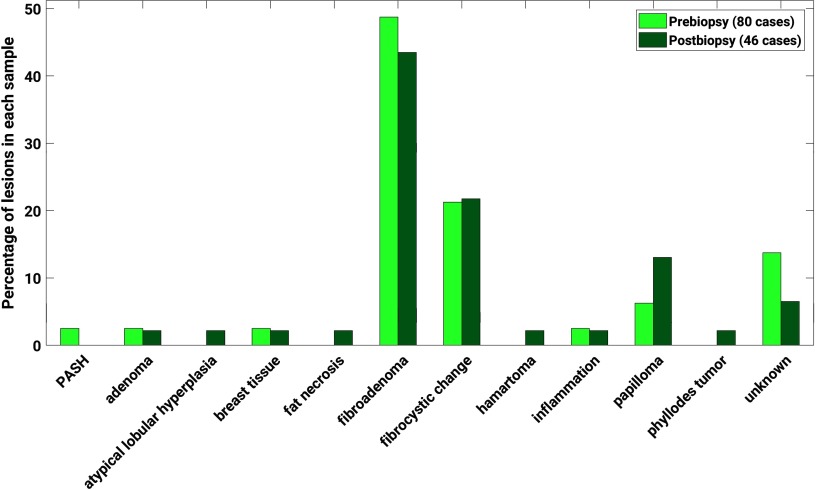
The benign lesions were comprised of a variety of subtypes according to pathology reports (Fig. 1).
Fig. 1.
Distribution of benign lesions by subtype, according to pathology reports. Fibroadenomas comprised 49% and 43% of the benign lesions imaged prebiopsy and postbiopsy, respectively, and 21% and 22% of each sample, respectively, were characterized by fibrocystic change. Subtype information was not available from pathology reports for and 7% of the benign lesions imaged prebiopsy and postbiopsy, respectively.
The voxel size varied between the MR images, but for most lesions (86% and 85% of benign lesions imaged pre- and postbiopsy, respectively, and 97% and 94% of luminal A cancers imaged pre- and postbiopsy, respectively), the voxel size was between 1 and . To assess the impact of voxel size in the study, the voxel size distribution was compared between lesion types for each biopsy condition, using the Kolmogorov–Smirnov test9,10 to determine whether the two groups being compared were drawn from the same distribution.
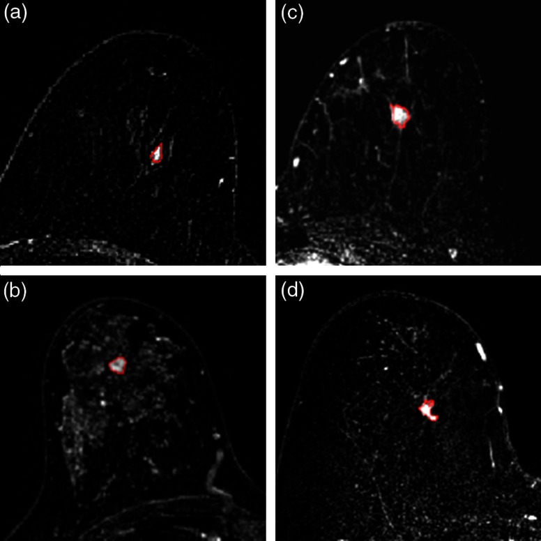
The lesions were automatically segmented using a fuzzy C-means method requiring only the manual indication of a seed-point inside the lesion (Fig. 2).11
Fig. 2.
Four example images from the dataset, with segmentation indicated by red lines. (a) Benign lesion imaged prebiopsy. (b) Benign lesion imaged postbiopsy. (c) Luminal A cancer imaged prebiopsy. (d) Luminal A cancer imaged postbiopsy.
Thirty-eight quantitative radiomic features describing the categories of size, shape, and morphology,12 texture enhancement,13 and kinetic curve assessment and enhancement variance kinetics14 were extracted automatically from the MR images of the lesions (Table 2). Size features of the groups of lesions were calculated and reported below but were excluded from statistical analysis and conclusions because we were interested in the impact of biopsy on features other than size. Moreover, in a previous study, a radiomic signature for the classification of benign lesions and luminal A breast cancers that excluded size features obtained performance equivalent to that of a signature that included size.15 Thus, the work described here involves comparison of 34 nonsize features.
Table 2.
Radiomic feature names and descriptions. Size features (designated by abbreviations S1, S2, S3, and S4) are included for reference, but the statistical analysis was not performed using these features.
| Image feature | Feature description | Reference |
|---|---|---|
| Volume () (S1) | Volume of lesion | [12] |
| Effective diameter (mm) (S2) | Greatest dimension of a sphere with the same volume as the lesion | |
| Surface area () (S3) | Lesion surface area | |
| Maximum linear size (mm) (S4) | Maximum distance between any two voxels in the lesion | |
| Sphericity (G1) | Similarity of the lesion shape to a sphere | |
| Irregularity (G2) | Deviation of the lesion surface from the surface of a sphere | |
| Surface area/volume (1/mm) (G3) | Ratio of surface area to volume | |
| Margin sharpness (M1) | Mean of the image gradient at the lesion margin | |
| Variance of margin sharpness (M2) | Variance of the image gradient at the lesion margin | |
| Variance of radial gradient histogram (M3) |
Degree to which the enhancement structure extends in a radial pattern originating from the center of the lesion |
|
| Contrast (T1) | Location image variations | [13] |
| Correlation (T2) | Image linearity | |
| Difference entropy (T3) | Randomness of the difference of neighboring voxels’ gray-levels | |
| Difference variance (T4) | Variations of difference of gray-levels between voxel-pairs | |
| Energy (T5) | Image homogeneity | |
| Entropy (T6) | Randomness of the gray-levels | |
| Inverse difference moment (homogeneity) (T7) | Image homogeneity | |
| Information measure of correlation 1 (T8) | Nonlinear gray-level dependence | |
| Information measure of correlation 2 (T9) | Nonlinear gray-level dependence | |
| Maximum correlation coefficient (T10) | Nonlinear gray-level dependence | |
| Sum average (T11) | Overall brightness | |
| Sum entropy (T12) | Randomness of the sum of gray-levels of neighboring voxels | |
| Sum variance (T13) | Spread in the sum of the gray-levels of voxel-pairs distribution | |
| Sum of squares (variance) (T14) |
Spread in the gray-level distribution |
|
| Maximum enhancement (K1) | Maximum contrast enhancement | [14] |
| Time to peak (s) (K2) | Time at which the maximum enhancement occurs | |
| Uptake rate (1/s) (K3) | Uptake speed of the contrast enhancement | |
| Washout rate (1/s) (K4) | Washout speed of the contrast enhancement | |
| Curve shape index (K5) | Difference between late and early enhancement | |
| Enhancement at first postcontrast time point (K6) | Enhancement at first postcontrast time point | |
| Signal enhancement ratio (K7) | Ratio of initial enhancement-to-overall enhancement | |
| Volume of most enhancing voxels () (K8) | Volume of the most enhancing voxels | |
| Total rate variation () (K9) | How rapidly the contrast will enter and exit from the lesion | |
| Normalized total rate variation () (K10) | How rapidly the contrast will enter and exit from the lesion | |
| Maximum enhancement-variance (E1) | Maximum spatial variance of contrast enhancement over time | |
| Enhancement-variance time to peak (s) (E2) | Time at which the maximum variance occurs | |
| Enhancement variance-increasing rate (1/s) (E3) | Rate of increase of the enhancement-variance during uptake | |
| Enhancement-variance decreasing rate (1/s) (E4) | Rate of decrease of the enhancement-variance during washout |
We performed two types of analyses: the first investigating the distribution of feature values and the second one investigating classification performance of individual features in the task of distinguishing between benign breast lesions and molecular subtype luminal A breast cancers.
In the first analysis, the first step was to visually compare feature values for all four lesion groups: benign prebiopsy, benign postbiopsy, luminal A prebiopsy, and luminal A postbiopsy. For visualization purposes, for each feature the values were normalized to with a range between 0 and 1 through
where and are the minimum and maximum values for that feature for the entire set of lesions, respectively. The second step was to quantitatively compare feature values for the two lesion types, i.e., separately for benign and for luminal A lesion types, by biopsy condition using the Kolmogorov–Smirnov test9,10 to determine whether the two groups being compared were drawn from the same distribution. For each feature, the feature value distribution for the benign prebiopsy group was compared to that for the benign postbiopsy group and the distribution for the luminal A prebiopsy group was compared to that for the luminal A postbiopsy group. This was done to assess whether biopsy had a significant effect on feature value distributions. Because of the number of comparisons ( features), the Bonferroni–Holm correction16 was applied to features only when the -value for the Kolmogorov–Smirnov test was less than 0.05. For these features, we adjusted the significance level for each feature based on a significance level for a single comparison. If for a given feature, for a given lesion type, the -value from the Kolmogorov–Smirnov test was less than its adjusted significance level, the feature failed to demonstrate a statistical significant difference between pre- and postbiopsy conditions and was considered to be potentially robust with respect to biopsy condition for that lesion type.
In the second analysis, the classification performance in the task of distinguishing benign versus luminal A lesions was compared by biopsy condition, that is, for each feature the classification performance for the prebiopsy condition was compared to that for the postbiopsy condition. This was accomplished using two methods. First, the area under the receiver operating characteristic curve17 (AUCROC) served as a performance metric and was estimated from the nonparametric Wilcoxon area. Bootstrapping (2000 iterations) was used to determine, for each feature, the confidence interval of AUCROC for each biopsy condition and the confidence interval of the difference in AUCROC () between biopsy conditions. Features for which classification outperformed random guessing for both biopsy conditions, i.e., the 95% confidence interval of the AUCROC did not include for both the pre- and postbiopsy groups, were considered potentially robust. For these, we assessed whether (1) there was a statistically significant difference in AUCROC between biopsy conditions (two-tailed test) and (2) whether we could demonstrate equivalence by biopsy condition for those features failing to demonstrate a statistical significance between biopsy conditions (two-tailed test). For the features outperforming random guessing, the Bonferroni–Holm correction was used to adjust the significance level of the -value and corresponding confidence interval for the difference in AUCROC () by biopsy condition relative to . For example, an adjusted significance level corresponded to a two-sided 97.5% confidence interval in superiority and equivalence testing. The equivalence margin has not been established for evaluating the equivalence of AUCROC in radiomics or computer-aided diagnosis, let alone radiology at large,18 so we evaluated similarity prima facie with an equivalence margin of 0.1.
As a supplement to the second analysis, we investigated the area under the precision–recall curve (AUCPRC) as an auxiliary performance metric (see Sec. 5 Appendix) for the features that outperformed random guessing for both biopsy conditions according to AUCROC. Although the AUCROC is insensitive to prevalence,17 precision, as an alternative measure of accuracy that depends on the number of true positives and false positives in a group, is sensitive to it.19
Finally, as a pilot study, we investigated the effect of magnet strength on the identification of potentially robust features by completing the analysis described above separately by field strength. The difference in magnet field strength itself may provide variations that affect the kinetic curve assessment and enhancement variance features.20,21 In addition, enhancement texture features (calculated at the first post-contrast DCE time point) may be affected by the accompanying differences in image resolution that are tied to differences in imaging protocols at different field strengths, although not inherently.22,23
A summary of the feature extraction and analysis pipeline is shown in Fig. 3.
Fig. 3.
Schematic of the workflow for the extraction and evaluation of radiomic features from DCE-MR images.
3. Results
3.1. Differences in Voxel Size
The voxel size distributions failed to demonstrate significant difference when compared between lesion types for a given biopsy condition, according to the Kolmogorov–Smirnov test to determine whether the two groups being compared were drawn from the same distribution. For lesions imaged prebiopsy, the -value from the Kolmogorov–Smirnov test to compare voxel size was 0.051, while for lesions imaged postbiopsy, the -value was 0.86.
3.2. Feature Value Distributions
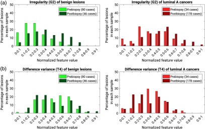
An example distribution of normalized feature values for each lesion type (benign or luminal A) by condition with respect to biopsy condition (prebiopsy or postbiopsy) is shown for two features (irregularity and difference variance) in Fig. 4.
Fig. 4.
Examples of distributions of normalized feature values for each lesion type by biopsy condition: (a) irregularity and (b) difference variance.
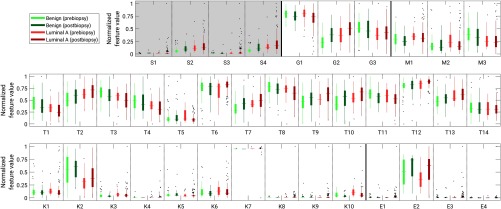
Distributions for all features using box plots of normalized feature values for each lesion type (benign or luminal A) by condition with respect to biopsy (prebiopsy or postbiopsy) are shown in Fig. 5. Visual inspection shows for some features large differences in the median values of both lesion types by biopsy condition, for example the irregularity (G2) of benign lesions and luminal A cancers compared pre- and postbiopsy. Some features show a wide range of values in one biopsy condition but not the other; for example, the texture features of energy (T5) and entropy (T6), for which the range of feature values for luminal A cancers imaged postbiopsy is much smaller than for luminal A cancers imaged prebiopsy.
Fig. 5.
Box plots of normalized feature values for benign (green bars) and luminal A lesions (red bars) from DCE-MR image series acquired either pre- or postbiopsy. The horizontal lines within the boxes indicate the median of a set, while the edges of the boxes indicate the 25th and 75th percentiles. The thin vertical lines for each box indicate the range of data values that are not considered outliers. The dots indicate outliers. Dashed vertical lines are drawn to separate each set of four groups of features by lesion status and biopsy conditions for a given feature, while solid vertical lines are drawn to indicate groups of features by category. Normalized values for size features are shown within a shaded box but were not included in statistical analysis. (S, size features; G, shape features; M, morphology features; T, enhancement texture features; K, kinetic curve assessment features; E, enhancement-variance kinetics). Full feature names are given in Table 2.
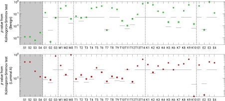
Using adjusted significance levels from Bonferroni–Holm multiple comparison testing and -values from the Kolmogorov–Smirnov test, most features failed to demonstrate a significant difference in their distribution between the prebiopsy and postbiopsy conditions (Fig. 6), suggesting that the occurrence of a biopsy event did not impact most of the extracted feature values. For benign lesions, the features of irregularity (G2), inverse difference moment (T7), and enhancement variance time to peak (E2) demonstrated significant differences in the distribution of feature values between the pre- and postbiopsy conditions. For luminal A lesions, the features of normalized total rate variation (K10) and enhancement variance time to peak (E2) demonstrated significant differences in distribution of feature values between pre- and postbiopsy conditions.
Fig. 6.
-values for the Kolmogorov–Smirnov test comparing the distributions of extracted feature values for benign (green) and luminal A lesions (red) by biopsy condition. The solid horizontal lines indicate the significance level each feature, for and otherwise according to the Bonferroni–Holm correction for multiple comparisons. Squares indicate a feature for which according to the Kolmogorov–Smirnov test but there was failure to demonstrate significant difference after correction for multiple comparisons. Stars indicate features for which a statistically significant difference was observed. Size features are shown within a shaded box but were not included in statistical analysis. Full feature names are given in Table 2.
3.3. Classification Performance
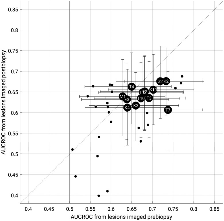
For the classification task of distinguishing between benign lesions and luminal A breast cancers for each biopsy condition, 14 features outperformed random guessing for both biopsy conditions as assessed by AUCROC (Fig. 7).
Fig. 7.
AUCROC for features extracted from images acquired postbiopsy versus those extracted from images acquired prebiopsy, in the task of distinguishing between benign lesions and luminal A breast cancers. The data points indicate the median value (2000 bootstrap iterations). Large black circles with feature abbreviations represent those that outperformed random guessing for both biopsy conditions. The data points for T1, T2, and T13 overlap in the figure. Error bars represent 95% confidence intervals. Small circles represent features which did not outperform random guessing for both biopsy conditions, and their error bars are not shown for figure clarity. The solid vertical and horizontal lines indicate (random guessing). Full feature names are given in Table 2.
For all features outperforming random guessing classification according to AUCROC, we failed to find a statistically significant difference in AUCROC between biopsy conditions. However, using the equivalence margin of 0.1, we were unable to demonstrate equivalence in AUCROC between the biopsy conditions. According to the AUCPRC metric, most features that outperformed random guessing according to the AUCROC metric performed better than baseline (i.e., cancer prevalence), the comparison for random guessing for precision–recall curves (see Sec. 5 Appendix).
3.4. Evaluation by Field Strength
When lesions were separated by field strength, results in feature distributions and classification performance differed. For benign lesions, the feature of normalized total rate variation (K10) and for luminal A cancers the features of energy (T5), entropy (T6), sum entropy (T12) demonstrated significant difference in feature value distribution when compared across biopsy condition for lesions imaged at 1.5 T. Additionally, at this field strength, only five features demonstrated classification performance better than random guessing, according to AUCROC, but for these five, no features demonstrated significant difference in feature value distribution for either lesion type. For lesions imaged at 3.0 T, eight features demonstrated significant difference in feature value distributions for benign lesions and 19 features did so for luminal A lesions. Eight features demonstrated classification performance better than chance for both prebiopsy conditions, but all of these coincided with at least one feature which demonstrated significant difference in feature value distribution. However, because the separation of the dataset by field strength reduces the number of cases for each evaluation, these assessments may be affected by the relatively low sample sizes.
3.5. Summary of Results
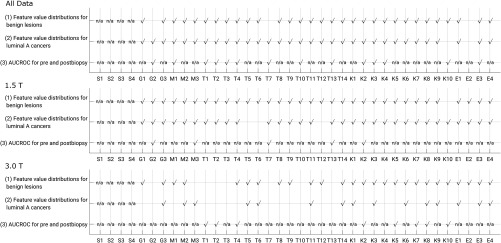
A summary of results for the tests of significant difference in nonsize feature value for each lesion type and of significant difference in AUCROC in the task of classification between benign lesions and luminal A cancers for features that performed better than chance, all compared by lesion status as pre- or postbiopsy, shows that all features of the lesions in the full dataset failed to demonstrate significant difference in both lesion value distributions and in AUCROC when compared against biopsy status (Fig. 8). The number of cases separated by field strength does not provide definitive insight into the classification performance of radiomic features by field strength within the context of biopsy condition of the lesions, but offers initial results on this issue.
Fig. 8.
Summary of statistical test results. Each comparison is made for groups of lesions by biopsy status. For each set, a check mark indicates that the feature distributions (rows 1 and 2) or difference in AUCROC (row 3) failed to demonstrate a statistically significant difference, and thus the feature may be robust. For the null-hypothesis for AUCROC comparison, only features with both for both biopsy conditions were assessed. Full feature names are given in Table 2.
4. Discussion and Conclusion
Most radiomic features of benign lesions and luminal A cancers failed to show a significant difference in their distribution of values when extracted from either pre- or postbiopsy images, indicating that the effects of biopsy on radiomic characterization may be minimal and that the features may be robust. The features that demonstrated significant differences in distribution of the feature values may have been affected because of disruptions in the lesion from the removal of tissue and the resulting effect on the intake and uptake of the contrast agent. One feature, enhancement-variance time to peak (E2), demonstrated significant difference in distribution of values in both groups of lesions, but this feature did not perform better than chance in the classification of lesions as benign or luminal A. In classification of benign lesions versus luminal A cancers, our results suggest that the introduction of the biopsy needle and/or clip failed to have a significant effect on the classification performance of those features that proved to be useful for classification, as measured by ROC curve performance (), suggesting that those features were potentially robust for the classification task by biopsy condition. The lack of demonstrable equivalence, however, limits the ability to absolutely affirm the robustness of features extracted from the lesions in this dataset. It is important to note that the irregularity of luminal A cancers has been shown to play an important role in their classification compared to benign lesions.15 In this study, the irregularity of benign lesions was significantly different between lesions imaged pre- or postbiopsy. The introduction of the biopsy needle and biopsy clip appears to disrupt the surface of the lesions, increasing their irregularity compared to other lesions that have not undergone biopsy; but in this study, this did not appear to have a significant effect on classification when considered separately by biopsy condition.
One limitation of this study is that the prevalence of luminal A lesions differs in each biopsy condition. To investigate the effect this could have on using a classification performance metric that is sensitive to the difference in prevalence, we investigated the AUCPRC; see the Sec. 5 Appendix for more information. As expected, because precision is dependent upon prevalence, the median AUCPRC was generally higher for these features in lesions imaged postbiopsy, compared to those that were imaged prebiopsy. However, this reflects the clinical nature of the dataset, influenced by typical scheduling of MR imaging and biopsy with respect to lesions first detected by, for example, mammography, versus high-risk screening programs involving MR imaging.
There could be variations in imaging protocol inherent to our dataset beyond image resolution. It is possible that there was variance in DCE-MR imaging protocol as a function of clinical contrast agent administration. For example, the dose of contrast agent may have been reduced for any patients with renal concerns. However, information regarding this was not available for our dataset. The relatively low numbers of cases when separated by field strength and the differences in prevalence between the groups by field strength limits the ability to comment conclusively on the differences in statistical conclusions when the lesions are separated in this manner, but is included for completeness. Because a different set of features performed better than random guessing according to AUCROC when the lesions were separated by field strength, further investigation into these differences is needed.
An additional area of limitation is that the cases in our study imaged under the pre- and postbiopsy condition were different, i.e., we did not have MR images of the same lesions imaged both pre- and postbiopsy, which would have increased statistical power. The number of cases was also limited by the selection of mass lesions only; our database did not have a sufficient number of nonmass enhancing lesions to be included in this study as a separate investigation. Our dataset also did not retain information that could identify the amount of time between prebiopsy and postbiopsy imaging, as these dates were removed as part of the patient anonymization process.
Our pilot study showed promising results regarding robustness of radiomic features by biopsy condition and more investigations are warranted using larger, preferably paired, datasets. The difference in robustness according to field strength and associated variables, such as associated differences in spatial resolution and how field strength itself can affect radiomic features related to contrast agent enhancement, is a topic of current investigation by our group. Future work will also expand analysis to cancers of different molecular subtypes.
5. Appendix
5.1. Methods
Due to the differences in cancer prevalence in the two biopsy-condition groups (30% for prebiopsy lesions, 79% for postbiopsy lesions), the AUCPRC was investigated as a complement to the assessment of classification performance using the receiver operating characteristic curve for features with AUCROC . When using precision–recall, the baseline performance in AUCPRC equals the disease prevalence (in our case, the prevalence of luminal A cancers) and represents random guessing, similar to 0.5 for AUCROC. Thus, AUCPRC classification performance with respect to the baseline was in the same manner as for AUCROC (2000 bootstrap iterations, using the same seeds for bootstrap sampling). We also assessed AUCPRC for a second subset with matched prevalence, drawn from the full sample. In this scenario, for each biopsy condition, the number of samples randomly drawn for each lesion type was limited to the size of the smallest set (i.e., the number of luminal A lesions imaged prebiopsy and the number of benign lesions postbiopsy).
5.2. Results
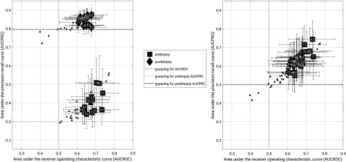
As expected, the AUCPRC for each group of lesions by biopsy condition differs in accordance with the difference in cancer prevalence (Fig. 9).
Fig. 9.
Classification performance in terms of AUCPRC versus AUCROC for (a) the full data set and (b) a subset of the data matched for prevalence during bootstrapping. The data points indicate the median value (2000 bootstrap iterations). The error bars represent the 95% confidence intervals. In each figure, squares represent prebiopsy lesions and diamonds represent postbiopsy lesions. The large, labeled data points represent features which performed better than random guessing according to AUCROC, while small, unlabeled points represent the remaining features and are shown for completeness. In (a), dotted and dashed horizontal lines represent baseline (e.g., random guessing) for AUCPRC in the prebiopsy and postbiopsy groups, respectively. In each figure, the vertical line represents random guessing for AUCROC. In (b), the baseline for each group is the same (0.5) and thus the horizontal lines overlap.
When the assessing the entire dataset, the AUCPRC was generally higher than the baseline performance level (baseline and for prebiopsy and postbiopsy conditions, respectively). For the prevalence-matched subsets, AUCPRC values clustered together and were generally greater than the equal baselines (baseline ). In this work, most features that performed better than guessing according to AUCROC did so as well according to AUCPRC, in both prevalence scenarios.
Acknowledgments
This work was funded in part by NIH U01 CA195564, NIH R15 CA227948, and the G.W. Aldeen Memorial Fund at Wheaton College. The authors gratefully acknowledge Dr. Ji Yu for discussions related to this work. Part of this work was presented at the International Workshop on Breast Imaging.
Biographies
Heather M. Whitney is an associate professor of physics at Wheaton College and a visiting scholar in the Department of Radiology, University of Chicago. Her experience in quantitative medical imaging has ranged from polymer gel dosimetry to radiation damping in nuclear magnetic resonance to now focusing on radiomics of breast cancer imaging. She is interested in investigating the effects of the physical basis of imaging on radiomics, as well as the repeatability and robustness of radiomics.
Karen Drukker is a research associate professor in the Department of Radiology, University of Chicago. She has been actively involved in computer-aided diagnosis/radiomics research for over a decade. Her work has focused on multimodality detection/diagnosis/prognosis of breast cancer and on the performance evaluation of radiomics methods.
Alexandra Edwards is a database specialist in the Department of Radiology, University of Chicago. She has expertise in the organization and implementation of quantitative image analyses and their associated multimodality datasets.
John Papaioannou is a computer scientist in the Department of Radiology, University of Chicago. He holds a master of science in computer science (computer vision) from Northwestern University. He has expertise in medical imaging database structuring and implementation, and has been instrumental in the computer-aided diagnosis and machine learning research in the Giger lab at the university.
Maryellen L. Giger is the A. N. Pritzker Professor of radiology and the Committee on Medical Physics at the University of Chicago. Her research entails the investigation of computer-aided diagnosis/radiomic/machine learning methods for the assessment of risk, diagnosis, prognosis, and response to therapy of breast cancer on multimodality (mammography, ultrasound, and magnetic resonance) images. She is also involved in the broad-based developments in computer vision and data mining of medical images.
Disclosures
MLG is a stockholder in R2 Technology/Hologic and a cofounder and equity holder in Quantitative Insights. MLG receives royalties from Hologic, GE Medical Systems, MEDIAN Technologies, Riverain Medical, Mitsubishi, and Toshiba. KD receives royalties from Hologic. It is the University of Chicago Conflict of Interest Policy that investigators disclose publicly actual or potential significant financial interest that would reasonably appear to be directly and significantly affected by the research activities.
References
- 1.Aerts H. J., et al. , “Decoding tumour phenotype by noninvasive imaging using a quantitative radiomics approach,” Nat. Commun. 5, 4006 (2014). 10.1038/ncomms5006 [DOI] [PMC free article] [PubMed] [Google Scholar]
- 2.Li H., et al. , “Quantitative MRI radiomics in the prediction of molecular classifications of breast cancer subtypes in the TCGA/TCIA data set,” Breast Cancer 2(1), 16012 (2016). 10.1038/npjbcancer.2016.12 [DOI] [PMC free article] [PubMed] [Google Scholar]
- 3.Burnside E. S., et al. , “Using computer-extracted image phenotypes from tumors on breast magnetic resonance imaging to predict breast cancer pathologic stage,” Cancer 122(5), 748–757 (2016). 10.1002/cncr.v122.5 [DOI] [PMC free article] [PubMed] [Google Scholar]
- 4.Sutton E. J., et al. , “Breast MRI radiomics: comparison of computer- and human-extracted imaging phenotypes,” Eur. Radiol. Exp. 1(1), 22 (2017). 10.1186/s41747-017-0025-2 [DOI] [PMC free article] [PubMed] [Google Scholar]
- 5.Cheung Y.-C., et al. , “Preoperative magnetic resonance imaging evaluation for breast cancers after sonographically guided core-needle biopsy: a comparison study,” Ann. Surg. Oncol. 11(8), 756–761 (2004). 10.1245/ASO.2004.12.008 [DOI] [PubMed] [Google Scholar]
- 6.Youngson B. J., Cranor M., Rosen P. P., “Epithelial displacement in surgical breast specimens following needling procedures,” Am. J. Surg. Pathol. 18(9), 896–903 (1994). 10.1097/00000478-199409000-00004 [DOI] [PubMed] [Google Scholar]
- 7.Layfield L. J., Frazier S., Schanzmeyer E., “Histomorphologic features of biopsy sites following excisional and core needle biopsies of the breast,” Breast J. 21(4), 370–376 (2015). 10.1111/tbj.2015.21.issue-4 [DOI] [PubMed] [Google Scholar]
- 8.Santiago L., et al. , “Breast cancer neoplastic seeding in the setting of image-guided needle biopsies of the breast,” Breast Cancer Res. Treat. 166(1), 29–39 (2017). 10.1007/s10549-017-4401-7 [DOI] [PubMed] [Google Scholar]
- 9.Kolmogorov A., “Sulla determinazione empirica di una legge di distributione,” G. dell’Istituto Ital. degli Attuari 4, 1–11 (1933). [Google Scholar]
- 10.Smirnov N., “Table for estimating the goodness of fit of empirical distributions,” Ann. Math. Stat. 19, 279–281 (1948). 10.1214/aoms/1177730256 [DOI] [Google Scholar]
- 11.Chen W., Giger M. L., Bick U., “A fuzzy C-means (FCM)-based approach for computerized segmentation of breast lesions in dynamic contrast-enhanced MR images,” Acad. Radiol. 13(1), 63–72 (2006). 10.1016/j.acra.2005.08.035 [DOI] [PubMed] [Google Scholar]
- 12.Gilhuijs K. G., Giger M. L., Bick U., “Computerized analysis of breast lesions in three dimensions using dynamic magnetic-resonance imaging,” Med. Phys. 25(9), 1647–1654 (1998). 10.1118/1.598345 [DOI] [PubMed] [Google Scholar]
- 13.Chen W., et al. , “Volumetric texture analysis of breast lesions on contrast-enhanced magnetic resonance images,” Magn. Reson. Med. 58(3), 562–571 (2007). 10.1002/(ISSN)1522-2594 [DOI] [PubMed] [Google Scholar]
- 14.Chen W., et al. , “Computerized interpretation of breast MRI: investigation of enhancement-variance dynamics,” Med. Phys. 31(5), 1076–1082 (2004). 10.1118/1.1695652 [DOI] [PubMed] [Google Scholar]
- 15.Whitney H. M., et al. , “Additive benefit of radiomics over size alone in the distinction between benign lesions and luminal A cancers on a large clinical breast MRI dataset,” Acad. Radiol. 26(2), 202–209 (2019). [DOI] [PMC free article] [PubMed] [Google Scholar]
- 16.Holm S., “A simple sequentially rejective multiple test procedure,” Scand. J. Stat. 6(2), 65–70 (1979). 10.2307/4615733 [DOI] [Google Scholar]
- 17.Metz C. E., “Basic principles of ROC analysis,” Semin. Nucl. Med. 8(4), 283–298 (1978). 10.1016/S0001-2998(78)80014-2 [DOI] [PubMed] [Google Scholar]
- 18.Ahn S., Park S. H., Lee K. H., “How to demonstrate similarity by using noninferiority and equivalence statistical testing in radiology research,” Radiology 267(2), 328–338 (2013). 10.1148/radiol.12120725 [DOI] [PubMed] [Google Scholar]
- 19.Garcia E. A., He H., “Learning from imbalanced data,” IEEE Trans. Knowl. Data Eng. 21(9), 1263–1284 (2009). 10.1109/TKDE.2008.239 [DOI] [Google Scholar]
- 20.Hittmair K., et al. , “Field strength dependence of MRI contrast enhancement: phantom measurements and application to dynamic breast imaging,” Br. J. Radiol. 69(819), 215–220 (1996). 10.1259/0007-1285-69-819-215 [DOI] [PubMed] [Google Scholar]
- 21.Rinck P., Muller R., “Field strength and dose dependence of contrast enhancement by gadolinium-based MR contrast agents,” Eur. Radiol. 9(1999), 998–1004 (1999). 10.1007/s003300050781 [DOI] [PubMed] [Google Scholar]
- 22.Mayerhoefer M. E., et al. , “Effects of MRI acquisition parameter variations and protocol heterogeneity on the results of texture analysis and pattern discrimination: an application-oriented study,” Med. Phys. 36(4), 1236–1243 (2009). 10.1118/1.3081408 [DOI] [PubMed] [Google Scholar]
- 23.Waugh S. A., et al. , “The influence of field strength and different clinical breast MRI protocols on the outcome of texture analysis using foam phantoms,” Med. Phys. 38(9), 5058–5066 (2011). 10.1118/1.3622605 [DOI] [PubMed] [Google Scholar]


