Developing a More Responsive Radiology Resident Dashboard

Abstract

Residents have a limited time to be trained. Although having a highly variable caseload should be beneficial for resident training, residents do not necessarily get a uniform distribution of cases. By developing a dashboard where residents and their attendings can track the procedures they have done and cases that they have seen, we hope to give residents a greater insight into their training and into where gaps in their training may be occurring. By taking advantage of modern advances in NLP techniques, we process medical records and generate statistics describing each resident’s progress so far. We have built the system described and its life within the NYP ecosystem. By creating better tracking, we hope that caseloads can be shifted to better close any individual gaps in training. One of the educational pain points for radiology residency is the assignment of cases to match a well-balanced curriculum. By illuminating the historical cases of a resident, we can better assign future cases for a better educational experience.

Background

Becoming a diagnostic radiologist in the USA requires 4 years of radiology-specific residency training during which residents are expected to become proficient with the breadth and depth of cases they will see throughout their career. On average, a radiology resident will see thousands of cases during their 4 years, but it is not necessarily true that residents will receive sufficient exposure across all classes of reads they will have to make [1]. Acknowledging the importance of experiential training and the staggering variety of cases in which radiologists need to be proficient, training programs have already taken steps to better track resident caseloads.

Radiology residencies in the UK have instituted logbooks that require residents to not only track the different cases they have worked up but ensure that they at least see a minimum number of cases across different classes [2]. Interventional radiology programs in the USA have also instituted similar logbooks for procedures. The existence of such practices demonstrates a demand for the ability for residents and residency programs to monitor caseloads.

With the digitization of medical records comes the ability to address such demands using data that is already being generated. While often maligned by physicians, electronic medical records (EMRs) have the potential, even if not fully realized, to improve physician and patient experience. By using this data, we allow residents insight into their own training and also how it compares against their peers. There have been prior examples [3] of computational tools to track effectiveness of medical education, but these tools often require sustained effort to collect and collate the required data sources. The popularization of EMRs provides an existing data pipeline to tap into which increases the sustainability of education tools that hook into this resource. There has already been some exploratory work done in the UK in this area to see how EMR data could automate parts of the resident logbook. However, even without explicit requirements to maintain such records in the USA, there appears to be value in providing our own residents such data given that it requires no extra human burden.

The Trove radiology resident dashboard is our attempt at an interactive, up-to-date, web-based dashboard that allows residents to visualize and track their case history, without the need for manual ingestion of data. Our hope is that by giving residents such a tool, we can empower them to direct their training to best prepare them for their future practice.

Medical records contain a significant amount of data in both structured and unstructured data formats. While there is a massive amount of nuanced information captured within unstructured clinician notes, our goal is to capture a summary of resident caseloads in broad brushstrokes. In that sense, structured data like ICD and CPT codes provide an ideal opportunity to take advantage of high-quality annotations that summarize provided care and are guaranteed to be part of all records. In contrast with other available forms of metadata like DICOM study names, ICD and CPT codes have the advantage of being standardized across institutions and capturing data related to diagnoses and patient type. These diagnoses and procedure codes are the data used by Trove to generate visualizations of resident case loads.

The drawback to this approach is that New York Presbyterian (NYP), like many other hospitals, outsources its coding which means that these codes are not available immediately. Because of this, there is a lag of up to a month before submitted codes get re-integrated into the EMR system. Because residency is finite, we understand that maximizing the utility of a dashboard like Trove includes improving its responsiveness.

To address this, we hoped to take advantage of advancements in machine learning to automate ICD/CPT classification, allowing the dashboard to provide up-to-date, albeit approximate, data around caseloads. There is a significant body of research around automating medical coding to reduce manual coding time by physicians or medical coders. So far, the research done around the automation of coding has been done on either a limited dataset or without using the latest advancements in machine learning technology [4–8]. There have been many advancements in machine learning for text processing along with statistical natural language processing that makes it a good time to work on this project.

Our problem-space has a couple of advantages compared to traditional automated coding systems, allowing us to put such an algorithm into production. First, our objective is not to create the final codes processed for billing. Rather, our goal is to generate codes as part of aggregate statistics around resident caseloads. As a result, while accuracy is important, perfect performance on each individual case is not required. Second, because we eventually get gold-standard human-annotated versions for all of our predicted codes, we have the opportunity for our algorithm to further train and improve itself over time. This type of setup is an example of iterative supervised training, a form of online learning, and is used for many production machine learning systems around the world.

Methods

Data Acquisition

In order to provide the end user with accurate and comprehensive information, Trove retrieves and integrates data from a variety of sources. The Trove study has been IRB approved at Weill Cornell Medical College. Our data access stream consists of a continuous HL7 dump from New York Presbyterian Hospital’s radiology records, which is then subsequently parsed and streamed to a mongoDB database using Mirth. The radiology records and associated metadata were obtained from 3 M’s CodeRyte dump and General Electric’s PACS system. Resident schedules were obtained manually using CSV dumps from Amion, a radiology resident scheduling system, and ingesting the data into our database.

Data Pipeline

Even though the continuous HL7 dump provides manual ICD and CPT codes, the information is not provided in real time. The overall turnaround time between report generation, medical coding, billing, and final validation from the payer can be on the order of weeks, particularly with cases of reimbursement denial. In order to provide more robust, real-time data for residents, Trove’s back-end uses state-of-the-art natural language processing (NLP) and neural network-based machine learning methods for predicting the codes on a radiology report before the gold standard is released. The system is expected to become more accurate at predicting codes as more and more data is processed through the system.

For the first iteration of Trove, only a subset of codes were analyzed and reported on the system, requested by radiology residents at New York Presbyterian Hospital, where the software was first deployed. The initial machine learning models were trained on data from 2004 to 2014 from ICD9 codes. The codes were then mapped to ICD10 equivalents for the purposes of the dashboard.

Preprocessing

Out of 2,185,643 radiology reports, we excluded all reports with no CPT code (n = 18,074), no ICD code (n = 63), or with a report length of less than 50 characters (n = 61).

All special characters and punctuation were removed from the report text. After running both Porter stemming and forgoing stemming, we made the decision to not stem individual words based on evaluation of the results. Words were tokenized, and words that appeared less than five times in the whole corpus were excluded. Finally, words from the SMART stoplist were excluded from our corpus [9].

Boolean Matching

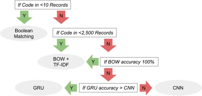
In situations where codes we wished to classify appeared less than 10 times in our dataset, we had no choice but to turn to exact term matching. In such cases, there is simply not enough training data to comfortably use a statistical model. Although we would rather avoid using rule-based approaches in our consensus model due to their lack of scalability, it was a tradeoff we were willing to make in order to classify all of the needed codes for our dashboard. There is also some intuition suggesting that this is not a bad approach for this subset of codes. We can reasonably expect to see less complex language structure when describing codes so specific that they appear less than 10 times in a dataset of over two million records. For example, we would not expect to see explicit negations in the text for an infrequently seen disease. In such cases, any mention of that specific disease is a strong indicator that the record should be tagged with that code.

Bag of Words and tf-idf

A bag of words (BOW) model is a popular model in natural language processing used for representing a body of text into a vector space model. The model discounts grammar and word ordering but takes into account presence and frequency of words. I is important to note that by dropping word ordering, it does not take into account negation of words. It also would struggle with a situation where the record says a patient has a “history of cancer,” and blindly looking for the word “cancer” could lead to misinterpreted results. Nevertheless, based on the literature, BOW models perform quite well in practice and are difficult to outperform.

As a baseline for evaluating more sophisticated models, we used a BOW model with term frequency-inverse document frequency (tf-idf) [10]. Tf-idf is often used as a weighting factor in text mining, natural language processing, and information retrieval uses. The underlying assumption in tf-idf is that the weight, or importance, of a term in a document is proportional to the term frequency, and that the specificity of a term can be quantified as an inverse function of the number of documents in which it occurs:

$$\mathit{\text{ft}},d$$

For the term frequency, we used the raw word count within a report. A report that mentions “pneumonia” multiple times is more likely to be related to pneumonia, for example. Other weighting schemes were evaluated, such as binary weighting and double normalization; however, raw counts performed the best:

$$\mathrm{idf}\left(t,D\right)=log\frac{N}{\mid \left\{d\in D:t\in d\right\}\mid }$$

Inverse document frequency was calculated using the formula above. A common word like “the” is likely to appear in all documents are down-weighted as such, while a highly specific word like “Budd-Chiari” is likely to be highly relevant and are up-weighted comparatively. Calculating tf-idf is calculated by an unweighted multiplication of the two terms above:

$$\text{tfidf}\left(t,d,D\right)=\mathrm{tf}\left(t,d\right)\cdot \mathrm{idf}\left(t,D\right)$$

A term-document matrix was calculated by calculating tf-idf for all terms in each radiology report. The collection of vectors was used for a simplistic single-layer perceptron model to evaluate a baseline.

Back-propagation with an Adam optimizer and early-stopping was performed. In evaluating the neural network, the negative class was down-sampled so there was an equal number of positive and negative cases.

Word Embeddings

One potential theoretical drawback to this method is the existence of synonymy, or multiple words having the same meaning (exopthalmos vs proptosis), and polysemy, or a single word having multiple meanings (trochlea). To address this, a popular computational linguistics technique is to evaluate words not in a naive vector space model, but in a reduced dimensionality space.

Common methods for accomplishing this are the use of latent semantic indexing (LSI), probabilistic latent semantic indexing (pLSI), or latent dirichlet allocation (LDA) [11–13]. Briefly, the methods above embed the entire vector space model into a substantially lower dimensionality, hoping to capture synonymy and polysemy and improve the quality of information retrieval. More recently, word embeddings were developed for this purpose for neural network use.

For Trove, we evaluated two state-of-the-art word-embedding methods, GloVe and Word2Vec [14, 15]. GloVe is based on a word-word co-occurrence model, while Word2Vec is based on a distributed representation of words based on continuous bag-of-words or a continuous skip-gram. After evaluating the performance of both GloVe and Word2Vec, we chose Word2Vec.

Raw word embedding models on a single-layer perceptron produced substantially worse results compared to our BOW benchmarks. However, in order to take into account negation and word order, dimensionality reduction and word embeddings is necessary. A 2 million-dimension word vector is too sparse, memory intensive, and cumbersome for state-of-the-art machine-learning methods.

Convolutional Neural Network

Convolutional neural networks (CNNs) are widely used in computer vision and image classification algorithms [16]. However, recently, they have seen increased use in natural language processing, even outperforming recurrent neural networks in classification tasks [17].

For our dataset, we used 1D convolutions with 128 × 5 kernel size and 1D max pooling with a length of 5. We used rectified linear units (RELUs) for activation of the convolutional layers and a dropout layer. RELUs and dropout are widely used in both natural language processing and computer vision problems. The parameters were obtained with an exhaustive grid search.

Because each kernel in the convolutional network is capable of identifying local context, word order and negation is theoretically considered in the machine-learning process. However, this method has drawbacks as well. It is impossible to capture large distances within the text. If a report references text from several sentences before, CNNs are unable to account for this. To deal with this drawback, variations on recurrent neural networks resistant to the vanishing gradient problem were considered.

Back-propagation with an Adam optimizer and early-stopping was performed. In evaluating the neural network, the negative class was down-sampled so there was an equal number of positive and negative cases.

Recurrent Neural Networks

To address the aforementioned problem, we used the latest advances in neural network-based approaches for NLP tasks: long short-term memory (LSTM) and gated recurrent unit (GRU)-based neural networks. LSTMs and GRUs are both units within a neural network that take advantage of “gated memory” in order to selectively “remember” relevant values over large spans of sequential data.

Each gated unit has a memory cell composed of an input gate, an output gate, and a forget gate. As such, it is capable of determining whether certain inputs are worth storing for a long period of time or a short period of time based on back-propagation results. In our final architecture, a standard GRU structure with forget gates was used, with gate equations shown below:

$$\begin{array}{c}\begin{array}{c}\begin{array}{c}{f}_t={\sigma }_g\left(W_{f{\chi }_t}+U_f{h}_{t-1}+b_f\right)\\ i_t={\sigma }_g\left(W_{i{\chi }_t}+U_i{h}_{t-1}+b_i\right)\end{array}\\ o_t={\sigma }_g\left(W_{o{\chi }_t}+U_o{h}_{t-1}+b_o\right)\end{array}\\ c_t=f_t\circ c_{t-1}+i_t\circ {\sigma }_c\left(W_{c{\chi }_t}+U_c{h}_{t-1}+b_c\right)\\ h_t=o_t\circ {\sigma }_h\left(\mathit{ct}\right)\end{array}$$

After evaluating the performance of LSTMs and GRUs, no significant differences were found. However, GRU’s had significantly faster performance, so they were used over LSTMs in the final architecture.

Back-propagation with an Adam optimizer and early-stopping was performed. In evaluating the neural network, the negative class was down-sampled so there was an equal number of positive and negative cases.

Consensus Model

Certain codes did not have enough training data. For codes with under 2500 positive cases, a simple rule-based system was used. We simply detected the presence of the disease name in the report and checked for an immediately preceding negation such as “history of,” “no signs of,” and so on.

Since certain models performed better than others for certain codes, we opted to use a consensus model. Consensus models are widely used in the literature for a variety of purposes, and an ensemble of models commonly outperforms any single model [18]. We deployed the models using Tensorflow Serving.

Web Architecture

The web server was written using Angular.js and node.js, with a mongoDB database. A number of wrapper features were engineered for visualization and gamification. Charts of the data were made using D3.js (Fig. 1).

Fig. 1.

Flowchart for model choice based on code characteristics

Results

Data Shape

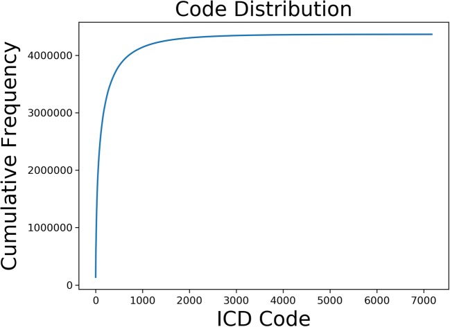
Figure 2 shows the cumulative frequency of codes used in our entire dataset. Note that the most frequent codes account for the vast majority of the dataset.

Fig. 2.

Cumulative frequency of most popular codes

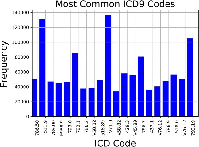
Figure 3 shows the most popular codes. In inspecting the most frequently used codes, several of the most frequent codes are non-descript, catch-all codes such as V71.9 “Observation for unspecified suspected condition”, or common constitutional symptoms such as 784.0 “headache.” Not all of these are valuable to resident education, and some of these findings are too common to be of use for tracking. Because of this, Trove subsamples only a small portion of our entire data and was curated based on resident needs.

Fig. 3.

Frequency of most popular ICD9 Codes

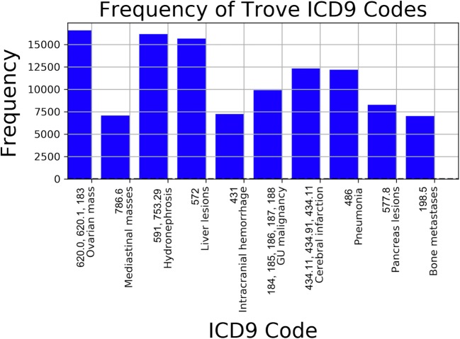
The actual codes deployed on Trove were comparatively less frequent, with common diagnoses such as “ovarian mass” accounting for the majority of total diagnoses and certain codes having no positive examples at all. The most common codes used in Trove are shown in Fig. 4.

Fig. 4.

Counts of most frequent codes used for Trove

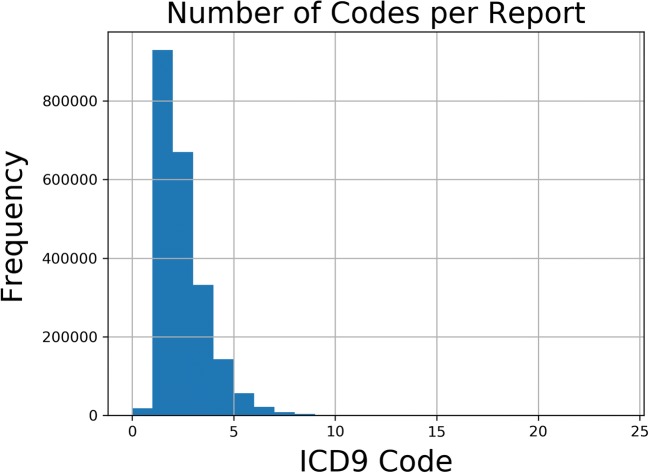
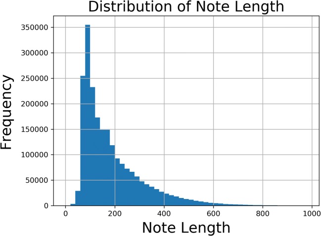
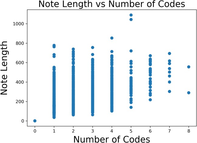
The classification problem is inherently multiclass. Figure 5 shows the distribution of number of codes per report. While the median number of codes per report is 1, multiple codes are not uncommon. There is also significant variability in the length of each note. Empirically speaking, there are some notes that follow a standard pattern or note a normal finding and others that are very long with multiple findings. Figure 6 shows the distribution of note length. Despite the variability in both number of codes per report and overall note length, there is only a loose correlation between note length and number of codes, as shown in Fig. 7.

Fig. 5.

Number of codes per report

Fig. 6.

Note length

Fig. 7.

Note length vs number of codes

Model Performance

Out of 227 codes that appeared in 10 records or more, 110 were perfectly classified by our BOW classifier. The average accuracy across those codes was 93.2%. However, if perfect scores were excluded from the dataset, accuracy drops to 86.7% on the remaining 117 codes. Looking only at non-perfectly classified codes appearing in greater than 2500 records (n = 28), the accuracy rises to 96.3% but is lower than both GRU and CNN accuracies across the same records.

Although our overall accuracy using either CNN or GRU architectures was lower than BOW, CNN or GRU architectures outperformed BOW for all except five codes when subsetting to codes found in greater than 2500 records and were not perfectly classified by BOW. Even for those five codes, BOW accuracy was only 0.46% better on average. The overall accuracy for CNN across the 28 codes that met this filter was 96.4 and 97.0% for GRU. This is a significant improvement compared to the 96.3% accuracy over the same codes using BOW.

Table 1 aggregates the findings listed above and lists the top 5 diagnoses for the three different models given. Lymphangiomyomatosis (LAM) is listed at the bottom as an example of one of the codes for the dashboards that fit the fallback criteria for Boolean matching.

Table 1.

Model performance across subsection of Trove codes

	Disease	Code	Training Size	Accuracy
				BOW	CNN	GRU	Consensus
Codes in > 2500 records	Tuberculosis	11	40,000	1.00	0.91	0.92	1.00
	Ascites or FAST	789.5	37,576	1.00	0.98	0.98	1.00
	Fibroids	218	35,466	1.00	0.99	0.99	1.00
	Pneumothorax...	512	32,164	1.00	0.99	0.99	1.00
	Gallstone	574	26,656	1.00	0.98	0.99	1.00
Codes in > 2500 records BOW Accuracy < 1.00	Hydronephrosis	591	22,906	0.96	0.99	0.97	0.99
	Liver lesions	573.8	20,994	0.96	0.96	0.97	0.97
	Pneumonia	486	19,298	0.95	0.98	0.99	0.99
	Cerebral infarction	434.91	17,588	0.97	0.98	0.97	0.98
	Ovarian cyst	620.2	16,844	0.98	0.99	0.99	0.99
Codes in < 2500 records	Pneumoperitoneum	568.89	2472	0.94	0.85	0.73	0.94
	Ovarian mass	620.9	2444	0.94	0.92	0.95	0.94
	Hardware complic...	996.4	2422	1.00	0.94	0.94	1.00
	Pancreatitis	577	2384	0.89	0.89	0.89	0.89
	Colitis	558	2350	1.00	0.91	0.95	1.00
Codes in < 10 records	Lymphangiomyomatosis (LAM)	516.4	8	N/A	N/A	N/A	N/A

Note that we did not use GRU for the Ovarian mass consensus model despite it having the highest overall score

Discussion

Model Discussion

Despite the strong assumption made by BOW that word order is irrelevant to the classification problem, the BOW classifier was our highest performing classifier. Overall, the BOW classifier performed extremely well. It is important to keep in mind that BOW, while ignoring word order, preserves the original data vocabulary. This gives BOW the capability to learn to exact-match multiple words even if it cannot exact-match sequences of words.

We hypothesize that the cases where BOW was not able to achieve 100% accuracy required preservation of word order in order to make the correct classification. The advantage and disadvantage of our deep learning approaches is that we feed the networks embeddings of the records using Word2Vec, trading vocabulary expressiveness for reduced sparsity. The disadvantage is that it becomes more difficult to exact-match words, likely the cause behind most of the BOW 100% accuracies. However, the advantage is that the reduction in sparsity allows us to feasibly train models that take into account language structure and can handle negations, misspellings, or multiple representations of concepts. It would make sense that codes that BOW is unable to achieve 100% accuracy on would be codes that require complex parsing, and therefore is consistent with the improved accuracy of the deep learning models for such codes. Based on these hypotheses, we manually inspected some of the records that were misclassified by BOW that were correctly classified by CNNs/GRUs to see if this was true. The results of this analysis are discussed in the Deep Dive on Classification Examples section.

We did not use deep-learning classifiers for codes appearing in less than 2500 records. Looking at our data, BOW significantly outperforms deep-learning approaches on such records. This makes sense given that deep-learning models require a significant amount of data to train. Although this means that our deep-learning models are currently being used for a minority of the codes we are classifying (n = 28), we believe this is the right approach for two reasons: (1) deep learning is not always the right choice for a problem. If a simpler model works well for a sub-classification task, use it because keeping it simple can avoid overfitting. (2) Our production models are trained in real-time because we continuously get codes for our records, albeit with a 1-month delay. This means eventually, all of our codes should have sufficient data for deep-learning approaches in the future.

Deep Dive on Classification Examples

Though the performance of GRUs and to a large extent, CNNs, are likely a “black box,” we can postulate several reasons for why they outperformed the BOW model in certain occasions. We believe that even though BOWs excelled when the classification task was simply recognizing the inclusion of a certain word, tasks of higher complexity required a more sophisticated model. To illustrate this point, we have picked some examples of trends that we found to be true for Trove.

First, words that are commonly negated, such as “pneumonia,” tended to have lower performance metrics when using BOW. This intuitively makes sense. BOW does not factor in word order and therefore may falsely assume that a document is about pneumonia even when it is negated. From manually inspecting classification results from the GRU model, we can see that this is the case. The GRU was able to correctly classify negation examples to a certain degree, such as “no evidence of pneumonia,” “clinically correlate to exclude pneumonia,” or even “atelectasis versus pneumonia,” in cases where the BOW marked them as false positives.

Extending the example further, the GRU was also able to correctly mark cases of pneumonia where the word pneumonia did not exist, such as in “...left lower lobe consolidation” or “near complete consolidation of the left lung.” As the word “consolidation” is commonly negated as well, it appeared that the BOW model had difficulty in classifying those cases as well. CNNs perform well in the case of negation. When considering “hydronephrosis,” CNNs performed the best and were able to correctly identify cases of negation such as in “no hydronephrosis, mass, or calculus” or “no left hydronephrosis.”

Second, GRUs excelled over BOWs when the challenge was to recognize a specific group of words. For “mediastinal mass,” for example, the BOW often reported false positives when the word “mediastinal” and “mass” were both in a document, but were not related. This is true in the document “The thyroid gland is symmetric without evidence of mass. Bilateral breast expanders are noted. Clips are seen within the right axilla. There is no axillary, mediastinal, or hilar adenopathy.” We found that CNNs and especially GRUs performed better in these cases.

Though this may be a shortcoming of not including bigrams, having bigrams and trigrams quickly makes the BOW model too sparse and unwieldy. Furthermore, the GRU was able to identify cases where the separation of words was rather large, as in the examples of “large soft tissue mass contain foci of calcification within the anterior mediastinum on the right” or “large heterogeneous mass in the medial right lung mildly extending into the right hilum and subcarinal region of the mediastinum”. N-grams are unlikely to solve the above issue, and CNNs also would not be able to capture such a large distance.

Finally, in cases where the disease cannot be explained by a clear set of words, such as “decreased gallbladder ejection fraction,” the BOW had substantially lower performance compared to GRUs and CNNs. The GRU was able to pick up on more subtle instances, such as “the gallbladder is again partially collapsed containing questionable sub-centimeter filling defects within the gallbladder fundus.” Intuitively, this makes sense, as a human would not be attempting to look for certain words in this case, but rather trying to interpret an underlying idea.

Notable Findings

Based on our work, we learned many valuable lessons. First, the quantity and quality of data is very important. We believe that we were able to achieve better metrics than those found in the literature, not because of heavy model optimization or the use of novel methods, but because our dataset was substantially bigger and cleaner.

In fact, for many codes, a simple bag of words classifier was not only sufficient but was able to provide perfect or near-perfect accuracy. However, for other codes, a more complex model was needed. For those codes, we were able to use more sophisticated models to take into account negation and word order.

Although our efforts were focused on a specialized case study on radiology reports, the techniques and findings can be used to inform many more problems in the medical community. From the architecture for the dashboard to the findings made about the feasibility of automated coding, we can extend this to any medical text that may benefit from NLP techniques for use in medical education.

Future Work

One direction of future research is to see, over the period of many years, the effect of implementing Trove. One intended outcome of Trove is the standardization of medical training, thereby encouraging residents to take on cases that they otherwise would not have seen. Interesting cases should be distributed somewhat equally throughout the residents’ workload instead of uniformly being distributed to one resident.

We can evaluate this by doing clustering based on individual residents in the past and using t-SNE or PCA to plot out the distribution of residents in their medical training. We can similarly then calculate the average distances between their respective caseloads. Ideally, with the implementation of Trove, such differences should decrease over time, as residents become exposed to more evenly distributed datasets.

Additionally, we hope to expand Trove’s reach to multiple teaching sites. It would be interesting to explore the differences in teaching between sites, and to be able to make recommendations to residents based on the results of findings made outside their immediate teaching facility. Furthermore, we can evaluate the challenges logistically of generalizing our platform, including integrating across multiple systems and supporting residents on different system architectures.

References

- 1.Bhargavan M, Kaye AH, Forman HP, Sunshine JH. Workload of radiologists in United States in 2006–2007 and trends since 1991–1992. Radiology. 2009;252(2):458–467. doi: 10.1148/radiol.2522081895. [DOI] [PubMed] [Google Scholar]
- 2.Willatt JMG, Mason AC. Comparison of radiology residency programs in ten countries. Eur Radiol. 2006;16(2):437–444. doi: 10.1007/s00330-004-2635-3. [DOI] [PubMed] [Google Scholar]
- 3.Denny JC, Smithers JD, Miller RA, Spickard A., III Understanding medical school curriculum content using KnowledgeMap. J Am Med Inform Assoc. 2003;10(4):351–362. doi: 10.1197/jamia.M1176. [DOI] [PMC free article] [PubMed] [Google Scholar]
- 4.Farkas R, Szarvas G. Automatic construction of rule-based ICD-9-CM coding systems. BMC Bioinformatics. 2008;9(Suppl. 3):S10. doi: 10.1186/1471-2105-9-S3-S10. [DOI] [PMC free article] [PubMed] [Google Scholar]
- 5.Pereira S, Névéol A, Massari P, Joubert M, Darmoni S. Construction of a semi-automated ICD-10 coding help system to optimize medical and economic coding. Stud Health Technol Inform. 2006;124:845–850. [PubMed] [Google Scholar]
- 6.Franz P, Zaiss A, Schulz S, Hahn U, Klar R. Automated coding of diagnoses--three methods compared. Proc AMIA Symp. 2000;2000:250–254. [PMC free article] [PubMed] [Google Scholar]
- 7.Lussier YA, Shagina L, Friedman C. Automating icd-9-cm encoding using medical language processing: A feasibility study. Proc AMIA Symp. 2000;2000:1072. [PMC free article] [PubMed] [Google Scholar]
- 8.Friedman C, Shagina L, Lussier Y, Hripcsak G. Automated encoding of clinical documents based on natural language processing. J Am Med Inform Assoc. 2004;11(5):392–402. doi: 10.1197/jamia.M1552. [DOI] [PMC free article] [PubMed] [Google Scholar]
- 9.Wibowo W, Williams HE: Simple and accurate feature selection for hierarchical categorisation. Proceedings of the 2002 ACM symposium on Document engineering 2002:111–118
- 10.Ramos J: Using tf-idf to determine word relevance in document queries. In: Proceedings of the first instructional conference on machine learning, 2003, 242:133–142
- 11.Deerwester S, Dumais ST, Furnas GW, Landauer TK, Harshman R. Indexing by latent semantic analysis. J Am Soc Inf Sci. 1990;41(6):391. doi: 10.1002/(SICI)1097-4571(199009)41:6<391::AID-ASI1>3.0.CO;2-9. [DOI] [Google Scholar]
- 12.Hofmann T. Probabilistic latent semantic indexing. ACM SIGIR Forum. 2017;51(2):211–218. doi: 10.1145/3130348.3130370. [DOI] [Google Scholar]
- 13.Blei DM, Ng AY, Jordan MI. Latent dirichlet allocation. J Mach Learn Res. 2003;3(Jan):993–1022. [Google Scholar]
- 14.Pennington J, Socher R, Manning C. Glove: Global vectors for word representation. Proc EMNLP Conf. 2014;2014:1532–1543. [Google Scholar]
- 15.Mikolov T, Sutskever I, Chen K, Corrado GS, Dean J. Distributed representations of words and phrases and their compositionality. Adv Neural Inf Proces Syst. 2013;26:3111–3119. [Google Scholar]
- 16.Krizhevsky A, Sutskever I, Hinton GE. Imagenet classification with deep convolutional neural networks. Adv Neural Inf Proces Syst. 2012;25:1097–1105. [Google Scholar]
- 17.Simard PY, Steinkraus D, Platt JC. Best practices for convolutional neural networks applied to visual document analysis. ICDAR. 2003;3:958–962. [Google Scholar]
- 18.Herrera F, Herrera-Viedma E. A model of consensus in group decision making under linguistic assessments. Fuzzy Sets Syst. 1996;78(1):73–87. doi: 10.1016/0165-0114(95)00107-7. [DOI] [Google Scholar]