Semi-intrusive multiscale metamodelling uncertainty quantification with application to a model of in-stent restenosis

Abstract

We explore the efficiency of a semi-intrusive uncertainty quantification (UQ) method for multiscale models as proposed by us in an earlier publication. We applied the multiscale metamodelling UQ method to a two-dimensional multiscale model for the wound healing response in a coronary artery after stenting (in-stent restenosis). The results obtained by the semi-intrusive method show a good match to those obtained by a black-box quasi-Monte Carlo method. Moreover, we significantly reduce the computational cost of the UQ. We conclude that the semi-intrusive metamodelling method is reliable and efficient, and can be applied to such complex models as the in-stent restenosis ISR2D model.

This article is part of the theme issue ‘Multiscale modelling, simulation and computing: from the desktop to the exascale’.

1. Introduction

Uncertainty quantification (UQ) of complex models is an increasingly important topic in computational biomedicine [1,2]. In order for computational models to be usable in practical applications, such as in silico medical trials and personalized medicine, the uncertainties in their predictions must be known. UQ methods compute these uncertainties as a function of uncertainty in the inputs (e.g. patient-specific parameter variability), taking into account any stochasticity in the model itself as well, i.e. model aleatoric uncertainty. However, these methods can be computationally expensive, especially when the model that requires a UQ analysis is computationally intensive itself. Reducing this computational burden is an important step on the way to production UQ of computationally expensive models such as in computational biomedicine.

UQ methods can be classified as intrusive or non-intrusive [3,4]. Intrusive methods, such as the Galerkin method [5], modify the model equations to directly propagate the uncertainties rather than a single model state. While often efficient, these methods do not immediately apply to all kinds of models. Moreover, if the model is highly nonlinear, intrusive methods may be expensive to compute. Non-intrusive methods use Monte Carlo algorithms, running the model many times with inputs sampled from a statistical distribution. This does not require changing the model and therefore applies universally, but it can be computationally expensive since a large number of (potentially themselves expensive) model runs are usually required.

Many complex simulation models are multiscale. They describe several interacting processes that take place at different scales in time and space [6–9]. For example, the in-stent restenosis (ISR) model described below models the response of blood flow patterns to changes in a diseased artery's geometry, a process that takes place in milliseconds, as well as the cell growth process that causes these changes and which may take weeks to complete. The implementation of such models usually consists of several computer programs that communicate with each other during the simulation, possibly via a coupling framework [9–11]. These multiscale simulations are often computationally expensive [12], and their UQ even more so. However, in some cases the multiscale nature of the model can be taken advantage of to improve performance of UQ. We refer to this as semi-intrusive UQ [4]. Semi-intrusive UQ of a multiscale simulation model substitutes a surrogate for the most expensive single-scale model in order to decrease the computational time of UQ, while preserving approximately correct estimation of the uncertainties. One example of semi-intrusive UQ is the metamodelling approach, where the micro model is replaced by a computationally cheaper surrogate model.

In this article, we describe the application of surrogate modelling to the UQ of a two-dimensional simulation of in-stent restenosis (ISR2D). ISR is the adverse reaction to angioplasty and stenting of stenosed arteries [13]. As this model is comparatively inexpensive to compute (unlike its three-dimensional variant [14]), we are able to compare the computational cost and accuracy of several surrogate models with those of a full quasi-Monte Carlo (QMC) UQ method [15].

2. ISR2D model

Cardiovascular diseases are the global leading cause of mortality [16]. Coronary artery stenosis is a widespread type of cardiovascular disease, in which the coronary artery is narrowed by the build-up of fatty plaque inside the artery. It is commonly treated by balloon angioplasty, which presses the plaque into the wall, followed by placement of a stent to keep the artery from collapsing. In 5–10% of cases, however, the injury caused by this procedure results in a renewed narrowing of the artery inside of the stent, due to abnormal growth of smooth muscle cells (SMCs) [13]. This is known as in-stent restenosis (ISR). Computer simulations of ISR may help to understand the causes of this process, and may in the future serve as a tool for in silico trials of, for example, improved stent designs.

(a). Model structure

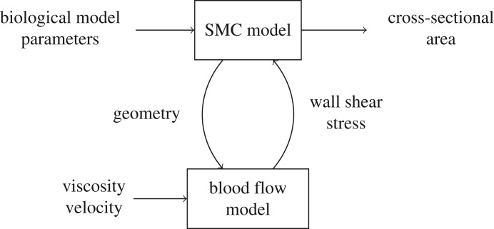
In this paper, we consider a two-dimensional simulation model of ISR [17]. We simplify it here to two submodels: a simulation of SMC growth into the artery lumen, and a simulation of blood flow through the artery (figure 1). SMC growth changes the geometry of the artery, which affects the blood flow, while the wall shear stress (WSS) caused by the blood flow inhibits SMC growth when it is above a threshold value. The final output of the model is the cross-sectional area of the neointima, which indicates the degree of restenosis. For a more detailed description of the model, we refer to previous papers [17–19].

Figure 1.

A multiscale model of in-stent restenosis.

Because the SMC growth process happens on much longer time scales than the response of the blood flow, ISR2D is a multiscale model, in particular a macro–micro model with separated time scales. For the implementation, this implies that the SMC model, which is the macro model, calls the blood flow model at each time step, sending it the current geometry of the artery. The blood flow model then runs to convergence, and returns the corresponding WSS pattern. When running on a single core for maximal computational efficiency, the blood flow model takes up ≈ 50–60% of the total run-time of the model. Therefore, replacing the blood flow model with a surrogate model has the potential to significantly increase performance of the overall simulation, but care must be taken that it does not significantly affect the accuracy of the results. For the three-dimensional simulations [14], our final target for the UQ, the time taken by the blood flow calculations is substantially higher. In order to obtain a closer approximation of the run-time characteristics of the three-dimensional model, we allocated four cores for the SMC model, while the real blood flow model as well as the surrogate models used a single core. This resulted in the SMC model using ≈ 15% of the wall clock time, with ≈ 85% used by the blood flow simulation.

The model is subject to aleatoric and epistemic uncertainty [15]. Aleatoric uncertainty is due to natural variability of the cell cycle, the relative orientation of daughter cells and the pattern of re-endothelialization in the SMC model [17,20]. Epistemic uncertainty is due to imperfect measurements of the values of the flow velocity, maximum deployment depth and endothelium regeneration time. The flow velocity is related to the blood flow model and is equal to the maximum velocity at the inlet. The other two parameters are related to the SMC model. Deployment depth is the difference between the initial position of the wall–lumen border and the final position of the outer side of stent struts. Endothelium regeneration time is the time until the endothelium is completely re-covered. We explore the effect of the model stochasticity and imprecision in the input values in the UQ study.

(b). Micro model input and output

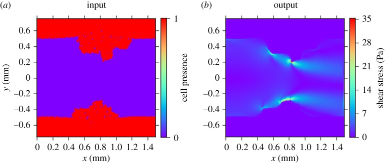
The input and output of the micro scale model (whether the actual blood flow model or a surrogate) are shown in figure 2. The inputs of the model are the geometry of a longitudinal section of the artery (figure 2a) and the maximum inlet velocity of the blood flow (not shown), and the output is the shear stress in the fluid (figure 2b). The domain measures 1.5 mm by 1.5 mm, with a grid spacing of 0.01 mm. Thus, we have a 150 by 150 binary grid plus a scalar as the input, and a 150 by 150 grid as the output.

Figure 2.

(a) Input (artery geometry, in red) and (b) output (shear stress) of the blood flow model.

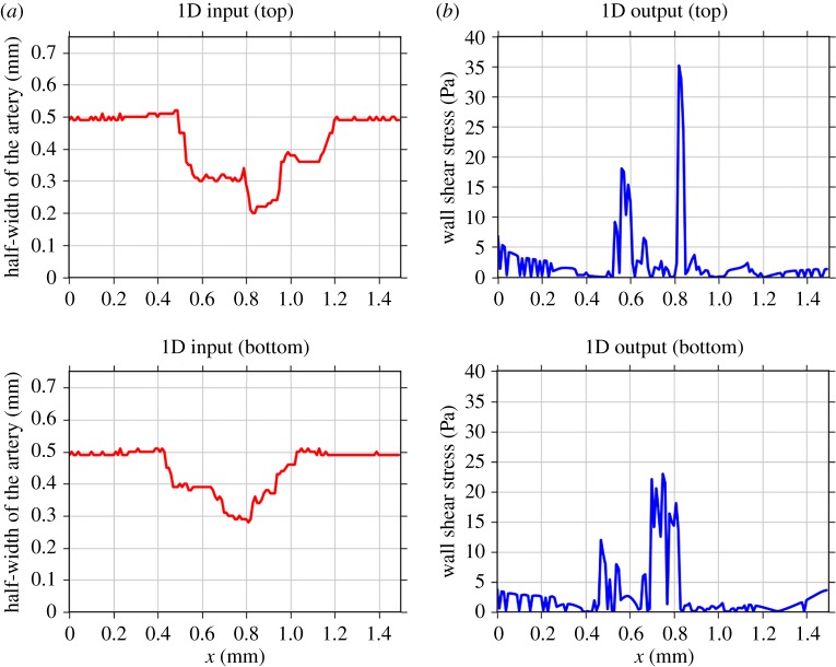
In order to build a surrogate, we first reduced the dimensionality of the inputs and outputs (figure 3). We converted the input grid to two vectors r^u(t) and r^l(t) containing the distances from the centre (y = 0) to the top or to the bottom lumen wall, where the half-width of the artery in figure 3a is computed by

$$\begin{array}{rl}{r}_x^u(t)& =(75-n_x^u(t))\times {10}^{-2}\hspace{0.17em}(\mathrm{mm})\\ \mathrm{and}{r}_x^l(t)& =(75-n_x^l(t))\times {10}^{-2}\hspace{0.17em}(\mathrm{mm}),\end{array}\}$$ 2.1

where n^u_x(t) and n^l_x(t) are the numbers of SMCs in column x (figure 2a) in the upper or lower part of the domain, respectively, at a simulation time t. Each of these vectors r^u and r^l are of size 150, i.e. r^u = (r^u₁ · sr^u₁₅₀) and r^l = (r^l₁ · sr^l₁₅₀), and we consider them as two separate inputs with the same blood flow velocity value. Correspondingly, we consider the top and bottom halves of the output separately.

Figure 3.

Converted input (a) and output (b) for the upper and lower halves of the flow domain, of the micro model to vectors of dimension 150. (Online version in colour.)

As the macro model uses only the shear stress value at the arterial wall, we similarly converted the original WSS output to two vectors of length 150 describing the shear stress at the top and bottom walls as a function of horizontal position (figure 3b).

3. Uncertainty quantification

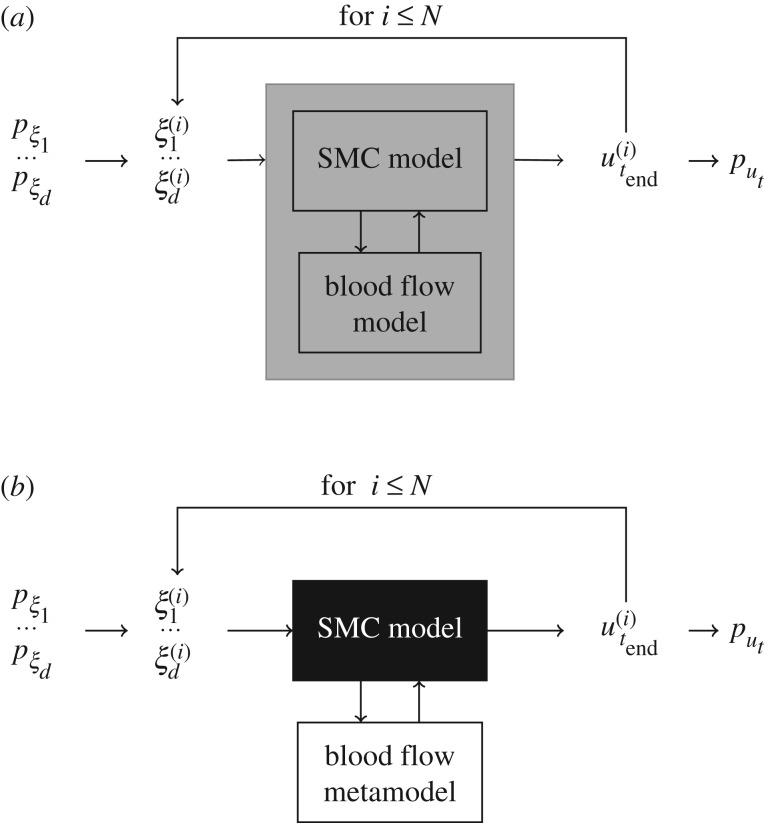
Monte Carlo (figure 4a) is a general and straightforward method for uncertainty propagation. However, if the model execution takes a significant amount of computational time, such methods can become prohibitively expensive. Since multiscale models are usually computationally demanding, we proposed a family of semi-intrusive UQ methods for multiscale models in [4].

Figure 4.

UQ methods: at each model run i, uncertain model inputs ξ_j (for 1 ≤ j ≤ d with d the number of inputs) take a value according to their distribution p_ξj, and a model result u⁽ⁱ⁾_{t end} is obtained. After collecting N outputs, the probability density function p_ut of model results is computed. In this work, d = 3 with ξ₁ flow velocity (m s⁻¹), ξ₂ maximum deployment depth (mm), ξ₃ endothelium regeneration time (days), and p_ξ1 = U(0.432, 0.528), p_ξ2 = U(0.09, 0.13), p_ξ3 = U(15, 23), where U(a, b) stands for a uniform distribution with [a, b] the range of possible values. The model response u_t is the cross-sectional area. (a) Black-box Monte Carlo and (b) semi-intrusive metamodelling approach.

In the metamodelling approach (figure 4b), the algorithm is similar to a usual Monte Carlo method, but instead of the original micro model there is a surrogate, obtained by building a simplified and computationally cheaper version of the model, or applying a data-driven approach using a collection of samples of size N_train. In this way, we approximate only the micro model function and keep the original macro model. When the sensitivity of the model's predictions to the output of the micro model is low, or when the metamodel mimics the result of the original micro model well, only a small error in the output will be introduced. And even more so, for UQ, where we are mainly interested in the average model output and its uncertainties, we could tolerate errors in the metamodel without too much influencing the estimates of the average model output and its uncertainties.

(a). Physical metamodel

We developed a metamodel based on a simplified representation of the fluid dynamics. In this model, we assume that the blood flow is a two-dimensional Poiseuille flow in a pipe. The WSS in this case is

$$\mathrm{WSS}=\frac{2\mu v}{r},$$ 3.1

where μ = 4 × 10⁻³ (Pa s) is the dynamic viscosity, v is the maximum velocity (m s⁻¹) and r is the radius of the pipe (m).

The simplified-physics metamodel assumes that fluid flow at any given point in the artery has such a parabolic profile, as if that slice of the artery was a slice of a long pipe with a diameter equal to the local width of the artery. Consequently, we calculated the distance from the centre to the upper or the lower artery wall r by equation (2.1), and then applied equation (3.1) to calculate the local WSS.

(b). Data-driven metamodel

The data-driven surrogate model predicts the WSS at a point in space x based on the nominal blood flow velocity, the local half-width of the channel (r_x), and the local shape of the channel represented by the vector

$$S_x=(r_x-r_{x-m},\dots ,r_x-r_{x-1},r_{x+1}-r_x,\dots ,r_{x+m}-r_x),$$

where for points past the edge of the domain, i.e. if x − i < 1 or x + i > 150, the value for r_x−i or r_x+i is set to equal r₀ or r₁₅₀, correspondingly. The choice of the number of neighbourhood points m is critical. If the value of m is close to 150, information on the geometry is preserved. On the other hand, if m is close to 0, the input dimensionality of the metamodel is low; therefore, the metamodel requires a lower training dataset and produces predictions in a shorter computational time.

In order to obtain training data, the ISR2D model was run N_train times with different values of the uncertain model inputs (as in figure 4a with N = N_train). At each simulation, the values of input and output of the blood flow model were saved, and then converted to one-dimensional vectors as described above.

For each coordinate x, the metamodel was trained using flow velocity, r_x′ and S_x′ from all recorded N_train runs corresponding to the current simulation time, where x′∈{x − n, …, x + n}. Using these n neighbour points as well increases the training sample size, resulting in better predictions. Thus, the total size of the training data for each metamodel was N_train(2n + 1).

Predictions were made using the nearest-neighbour interpolation method¹ with different values of m, N_train and n. After some initial experiments to determine reasonable values of these metamodel parameters, we built two data-driven metamodels with different settings, in order to study the trade-off between the computational requirements of collecting training data and the resulting prediction quality. Table 1 contains the settings we used in this work.

Table 1.

Settings for the two data-driven metamodels used in the study.

parameter	notation	DD metamodel 1	DD metamodel 2
number of inputs with the gradients to the left and right	m	10	5
training sample size	Ntrain	10	5
number of neighbour points in space to the left and to the right, which were used to increase the dataset	n	15	5

(c). Sampling

The reference solution by QMC was obtained by sampling 960 model results with different values of uncertain model inputs [15]. We followed the same sampling procedure for the metamodelling cases, collecting 960 samples for each case, with input parameters generated using a Sobol sequence. We used the Sobol library [22] to generate the Sobol quasi-random sequences [23].

4. Results

Here we present a comparison of computational performance and accuracy of the results obtained by the different UQ methods discussed above, as compared to the black-box Monte Carlo results [15].

Our main goal for the metamodelling method is to reduce the computational burden of a given model, in order to make UQ feasible. Figure 5 shows the time needed for a single model run using each of the four UQ methods: the quasi-Monte Carlo (QMC), the data-driven metamodels (DD meta I and II) with two different settings according to table 1, and the metamodelling by the simplified physical surrogate. The light colours indicate the total execution time of the whole multiscale model, and the dark colours indicate the portion of the time taken by the micro model or surrogate. For the metamodelling methods, the indicated time includes the construction of the metamodels. DD meta I reduces total run-time by almost half. DD meta II, which uses less data, is faster still, at five times the speed of the original. The physical metamodel is fastest, but only by a small margin over DD meta II.

Figure 5.

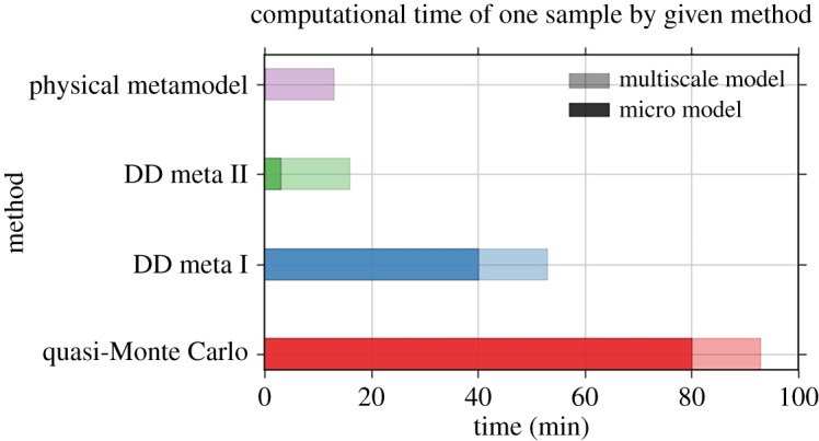
Comparison of the computational time per one model run with different UQ methods. (Online version in colour.)

Improved performance is only useful, however, if the results are still sufficiently accurate. Figure 6 contains the results of the uncertainty estimation (mean value and standard deviation) of the ISR2D model's output, the cross-sectional area of the neointima, by different UQ methods. The results show all metamodels producing less growth than the reference model, but there is still a large overlap in the estimated uncertainty areas. DD meta I, the slowest metamodel, is closest to the reference solution, and the faster DD meta II shows only a slightly worse result than DD meta I. The physical metamodel shows the largest deviation.

Figure 6.

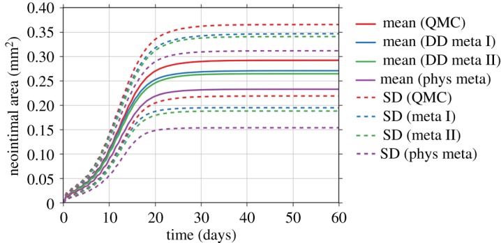
Comparison of the estimated mean and standard deviation (SD) by the quasi-Monte Carlo (QMC) method, metamodelling methods by data-driven (DD meta I and II) approach and by simplified physics (phys meta).

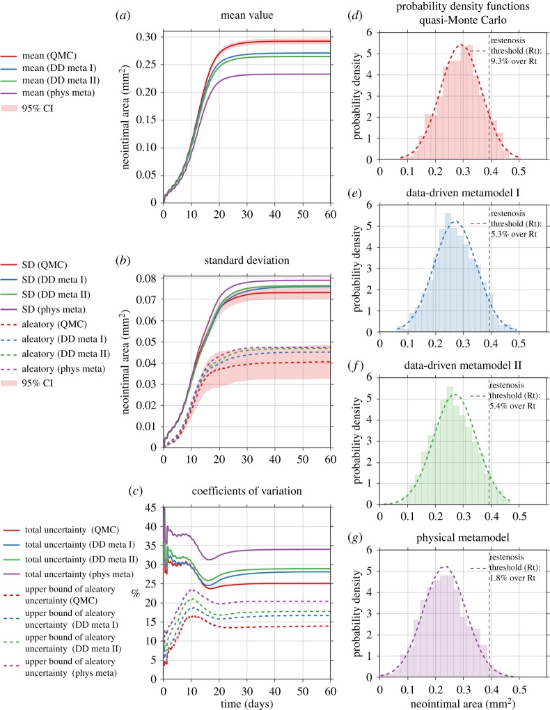
Figure 7 contains a more detailed analysis of the results obtained by the four UQ methods. Figure 7a shows the estimated mean value obtained from the four methods, with the 95% bootstrap confidence interval [24] plotted as a red shaded area around the results from the QMC method. All three metamodelling results show a statistically significant underestimation of the mean value (two-valued t-test, p < 0.01).

Figure 7.

Analysis of the uncertainty measures by the four UQ methods: the quasi-Monte Carlo (QMC) method, metamodelling methods by data-driven (DD meta I and II) approach and by simplified physics (phys meta).

ISR2D is subject to both epistemic and aleatoric uncertainty. Some model inputs are uncertain due to lack of knowledge, and the model is also stochastic itself because it simulates the natural variability of the process of interest. We estimated the total standard deviation, as well as an upper bound of the partial standard deviation due to aleatoric model uncertainty² . As figure 7b shows, the metamodelling estimates are high, but for the data-driven metamodels still within the 95% confidence interval of the QMC result.

The coefficients of variation (CoV) shown in figure 7c are equal to the ratio between the (partial) standard deviation and the mean value, and are a measure of the relative model output uncertainties. Here we observe that the underestimation of the mean value leads to the overestimation of the CoV.

Figure 7d–g shows the distribution of the cross-sectional areas at the final simulation time step. The dashed vertical line indicates a restenosis threshold, defined as 50% occlusion of the original lumen area [26]. Thus, about 9.7% out of all samples obtained by QMC result in restenosis. The data-driven metamodel results are about half this value. The results with the physical metamodel shows a result of only 1.8%, and a shift of the probability density function to the left is visible.

5. Discussion

Our results show that the metamodelling method for UQ can result in significant reduction of computational time in comparison with the black-box QMC method. Our fastest metamodel reduced the time taken by the blood flow calculations by a factor of 20, reducing the overall compute time by a factor of 5. For the three-dimensional version of the ISR model, the blood flow calculations take up a much larger fraction of the compute time, which would result in an even larger improvement. For computationally expensive three-dimensional multiscale models, our semi-intrusive multiscale UQ methods may be the only viable solution to perform UQ in a reasonable time frame, even if large-scale computing environments are available.

This performance improvement did result in reduced accuracy of the estimated mean values and uncertainties. We found a statistically significant lower mean cross-sectional area for all metamodels (p < 0.01), as well as larger standard deviations. The overall difference, although statistically significant, is fairly small, however, with the mean final cross-sectional area produced by the best metamodel only deviating by 7.3%, which is much less than the 25% overall uncertainty in the original model's output. The best final standard deviation differed by 3.8%. This result matches well with our previous results [15], which showed that the overall output of ISR2D is relatively insensitive to the output of the blood flow submodel. We hypothesize that our metamodelling approach to multiscale UQ can be very beneficial for those multiscale models where the sensitivity to the output of their micro scale model is relatively small, in comparison to sensitivities to the uncertain parameters in the rest of the multiscale model. We intend to explore this in more detail in future work.

Whether a given level of error is acceptable depends on the application. For ISR, ultimately what matters is whether a restenosis has occurred, as this necessitates further treatment. The estimated probability of this occurring, given the input parameters and their uncertainties, is 9.3% according to the original model, and 5.3% according to the best metamodel, a difference that would be considered too high in clinical practice.

This suggests that, in order to obtain an accurate UQ of a three-dimensional model of ISR, several challenges will have to be met. The metamodel needs to be improved to the point where the probability of restenosis can be estimated accurately, by improving the surrogate model structure, by using more training data, or by some kind of bias correction. For the three-dimensional version of the model, a further complication is that running a black-box QMC UQ is computationally very hard, so that the metamodel will have to be validated in a different way. In our previous work [4], we developed several semi-intrusive methods for UQ that can work under these constraints, and we plan to explore those in future work.

In conclusion, the semi-intrusive multiscale metamodelling is an efficient method to estimate uncertainty in the model response, when the model is composed of single-scale components. Moreover, the method can be standardized when it is applied in combination with the data-driven approaches, or can be a specific model together with simplified physics surrogate models.

Authors' contributions

A.N. and L.V. carried out the experiments. A.N. performed the data analysis. P.Z. and A.G.H. conceived of the work. A.N., L.V. and P.Z. designed the study and drafted the manuscript. A.G.H. supervised the study. All authors read and approved the manuscript.

Competing interests

The authors declare that they have no competing interests.

Funding

This work was supported by the Netherlands eScience Center under the e-MUSC (Enhancing Multiscale Computing with Sensitivity Analysis and Uncertainty Quantification) project. This project has received funding from the European Union Horizon 2020 research and innovation programme under grant agreement #800925 (VECMA project) and grant agreement #671564 (ComPat project). The authors acknowledge financial support by The Russian Science Foundation under agreement #14-11-00826. This work was sponsored by NWO Exacte Wetenschappen (Physical Sciences) for the use of supercomputer facilities, with financial support from the Nederlandse Organisatie voor Wetenschappelijk Onderzoek (Netherlands Organization for Science Research, NWO).

References

- 1.Mirams GR, Pathmanathan P, Gray RA, Challenor P, Clayton RH. 2016. Uncertainty and variability in computational and mathematical models of cardiac physiology. J. Physiol. 594, 6833–6847. ( 10.1113/tjp.2016.594.issue-23) [DOI] [PMC free article] [PubMed] [Google Scholar]
- 2.Brault A, Dumas L, Lucor D. 2017. Uncertainty quantification of inflow boundary condition and proximal arterial stiffness-coupled effect on pulse wave propagation in a vascular network. Int. J. Numer. Method Biomed. Eng. 33, e2859 ( 10.1002/cnm.2859) [DOI] [PubMed] [Google Scholar]
- 3.Smith RC. 2013. Uncertainty quantification: theory, implementation, and applications. Philadelphia, PA: SIAM. [Google Scholar]
- 4.Nikishova A, Hoekstra AG. 2018 Semi-intrusive uncertainty quantification for multiscale models. (http://arxiv.org/abs/1806.09341. ).
- 5.Mathelin L, Hussaini MY, Zang TA. 2005. Stochastic approaches to uncertainty quantification in CFD simulations. Numer. Algorithms. 38, 209–236. ( 10.1007/BF02810624) [DOI] [Google Scholar]
- 6.Sloot PMA, Hoekstra AG. 2010. Multi-scale modelling in computational biomedicine. Br. Bioinform. 11, 142–152. ( 10.1093/bib/bbp038) [DOI] [PubMed] [Google Scholar]
- 7.Weinan E. 2011. Principles of multiscale modeling. Cambridge, UK: Cambridge University Press. [Google Scholar]
- 8.Hoekstra AG, Chopard B, Coveney PV. 2014. Multiscale modelling and simulation: a position paper. Phil. Trans. R. Soc. A 372, 20130377 ( 10.1098/rsta.2013.0377) [DOI] [PubMed] [Google Scholar]
- 9.Chopard B, Borgdorff J, Hoekstra AG. 2014. A framework for multi-scale modelling. Phil. Trans. R. Soc. A 372, 20130378 ( 10.1098/rsta.2013.0378) [DOI] [PMC free article] [PubMed] [Google Scholar]
- 10.Chopard B, Falcone J-L, Kunzli P, Veen L, Hoekstra A. 2018. Multiscale modeling: recent progress and open questions. Multiscale Multidiscip. Model. Exp. Des. 1, 57–68. ( 10.1007/s41939-017-0006-4) [DOI] [Google Scholar]
- 11.Groen D, Knap J, Neumann P, Suleimenova D, Veen L, Leiter K. 2019. Mastering the scales: a survey on the benefits of multiscale computing software. Phil. Trans. R. Soc. A 377, 20180147 ( 10.1098/rsta.2018.0147) [DOI] [PMC free article] [PubMed] [Google Scholar]
- 12.Alowayyed S, Groen D, Coveney PV, Hoekstra AG. 2017. Multiscale computing in the exascale era. J. Comput. Sci. 22, 15–25. ( 10.1016/j.jocs.2017.07.004) [DOI] [Google Scholar]
- 13.Iqbal J, Gunn JP, Serruys PW. 2013. Coronary stents: historical development, current status and future directions. Br. Med. Bull. 106, 193–211. ( 10.1093/bmb/ldt009) [DOI] [PubMed] [Google Scholar]
- 14.Zun PS, Anikina T, Svitenkov A, Hoekstra AG. 2017. A comparison of fully-coupled 3D in-stent restenosis simulations to in-vivo data. Physiol. 8, 284 ( 10.3389/fphys.2017.00284) [DOI] [PMC free article] [PubMed] [Google Scholar]
- 15.Nikishova A, Veen L, Zun P, Hoekstra AG. 2018. Uncertainty quantification of a multiscale model for in-stent restenosis. Cardiovasc. Eng. Technol. 9, 761–774. ( 10.1007/s13239-018-00372-4) [DOI] [PMC free article] [PubMed] [Google Scholar]
- 16.World Health Organization 2018. Global health estimates 2016: Deaths by cause, age, sex, by country and by region, 2000–2016. Geneva, Switzerland: World Health Organization.
- 17.Caiazzo A. 2011. A complex automata approach for in-stent restenosis: two-dimensional multiscale modelling and simulations. J. Comput. Sci. 2, 9–17. ( 10.1016/j.jocs.2010.09.002) [DOI] [Google Scholar]
- 18.Evans DJW. et al. 2008. The application of multiscale modelling to the process of development and prevention of stenosis in a stented coronary artery. Phil. Trans. R. Soc. A 366, 3343–3360. ( 10.1098/rsta.2008.0081) [DOI] [PubMed] [Google Scholar]
- 19.Tahir H, Hoekstra A, Lorenz E, Lawford P, Hose D, Gunn J, Evans D. 2011. Multi-scale simulations of the dynamics of in-stent restenosis: impact of stent deployment and design. Interface Focus 1, 365–373. ( 10.1098/rsfs.2010.0024) [DOI] [PMC free article] [PubMed] [Google Scholar]
- 20.Tahir H, Bona-Casas C, Hoekstra AG. 2013. Modelling the effect of a functional endothelium on the development of in-stent restenosis. PLoS ONE 8, e66138 ( 10.1371/journal.pone.0066138) [DOI] [PMC free article] [PubMed] [Google Scholar]
- 21.Oliphant TE. 2007. Python for scientific computing. Comput. Sci. Eng. 9, 10–20. ( 10.1109/MCSE.2007.58) [DOI] [Google Scholar]
- 22.Chisari C. 2014. SOBOL. The Sobol quasirandom sequence (Python library for the Sobol quasirandom sequence generation). See http://people.sc.fsu.edu/%7Ejburkardt/py_src/sobol/sobol.html.
- 23.Sobol IM. 1998. On quasi-Monte Carlo integrations. Math. Comput. Simul. 47, 103–112. ( 10.1016/S0378-4754(98)00096-2) [DOI] [Google Scholar]
- 24.Archer GE, Saltelli A, Sobol IM. 1997. Sensitivity measures, ANOVA-like techniques and the use of bootstrap. J. Stat. Comput. Simul. 58, 99–120. ( 10.1080/00949659708811825) [DOI] [Google Scholar]
- 25.Saltelli A, Annoni P, Azzini I, Campolongo F, Ratto M, Tarantola S. 2010. Variance based sensitivity analysis of model output. Design and estimator for the total sensitivity index. Comput. Phys. Commun. 181, 259–270. ( 10.1016/j.cpc.2009.09.018) [DOI] [Google Scholar]
- 26.Serruys PW. et al. 2009. A bioabsorbable everolimus-eluting coronary stent system (ABSORB): 2-year outcomes and results from multiple imaging methods. Lancet 373, 897–910. ( 10.1016/S0140-6736(09)60325-1) [DOI] [PubMed] [Google Scholar]
- 27.Bal H, Epema D, de Laat C, van Nieuwpoort R, Romein J, Seinstra F, Snoek C, Wijshoff H. 2016. A medium-scale distributed system for computer science research: infrastructure for the long term. Computer 49, 54–63. ( 10.1109/MC.2016.127) [DOI] [Google Scholar]