Global Seismic Nowcasting With Shannon Information Entropy

Abstract

Seismic nowcasting uses counts of small earthquakes as proxy data to estimate the current dynamical state of an earthquake fault system. The result is an earthquake potential score that characterizes the current state of progress of a defined geographic region through its nominal earthquake “cycle.” The count of small earthquakes since the last large earthquake is the natural time that has elapsed since the last large earthquake (Varotsos et al., 2006, https://doi.org/10.1103/PhysRevE.74.021123). In addition to natural time, earthquake sequences can also be analyzed using Shannon information entropy (“information”), an idea that was pioneered by Shannon (1948, https://doi.org/10.1002/j.1538‐7305.1948.tb01338.x). As a first step to add seismic information entropy into the nowcasting method, we incorporate magnitude information into the natural time counts by using event self‐information. We find in this first application of seismic information entropy that the earthquake potential score values are similar to the values using only natural time. However, other characteristics of earthquake sequences, including the interevent time intervals, or the departure of higher magnitude events from the magnitude‐frequency scaling line, may contain additional information.

Key Points

• Nowcasting was previously used to analyze earthquake data to determine current seismic risk to global megacities for magnitudes M ≥ 6

• We extend the method to computing hazard from great earthquake and mega‐tsunami sources arising from earthquakes with magnitudes M > 7.9

• We also develop nowcasting methods using the information entropy of earthquake sequences

1. Introduction

The determination of earthquake risk for geographic regions is an old problem that has been associated with the development of methods for forecasting and prediction (Holliday et al., 2016; Scholz, 2002; WGCEP [http://www.wgcep.org/overview]). In many ways, the problem of earthquake forecasting bears similarities to the problem of forecasting in weather and economic systems (Jolliffe & Stephenson, 2003; OECD [http://www.oecd.org/economy/oecd‐forecasts‐during‐and‐after‐the‐financial‐crisis‐a‐post‐mortem.htm]). In all these cases, probabilities of future activity are calculated using physical or statistical models and then validated by backtesting and prospective testing.

An associated question is the degree to which past and present conditions convey information about future conditions. For the case of weather forecasting, the continual improvement of forecasting methods is evidence that there is considerable information contained in past data and that the improvement of data acquisition via satellite observations maps into better probabilities of future activity (Marshall et al., 2006).

An important goal is therefore to quantify the amount of information that is contained in past activity. In order to address this question, we begin with the simpler idea of nowcasting and apply ideas from the field of statistical communication theory (Shannon information entropy). Nowcasting is a simpler form of risk estimation than forecasting and is therefore readily amenable to analysis of information content.

2. Nowcasting

Nowcasting refers to the use of proxy data to estimate the current dynamical state of a driven complex system such as earthquakes, neural networks, or the financial markets (Rundle et al., 2016). In previous papers (Rundle et al., 2016; Rundle et al., 2018), a method to nowcast earthquakes has been presented based on the natural time count of small earthquakes after the last large earthquake in a defined, seismically active geographic region. Natural time has been discussed extensively in Varotsos et al. (2004, 2005, 2006), Sarlis et al. (2011, 2018), Vallianatos et al. (2012), and Holliday et al. (2006).

The basic idea is that the recurring pattern, or cycle, of “large earthquake‐quiescence‐large earthquake” is characterized by an “earthquake clock” that in some way quantitatively describes the region (e.g., Hill & Prejean, 2007; Rogerson, 2018). Nowcasting is a method that can be used to statistically define the current state of this earthquake clock.

In the nowcasting method, a “large” seismically active geographic region is identified in which a “local” region of interest is embedded. The primary assumption in the method is that the frequency‐magnitude statistics of the large region are the same as the those of the local region. From a practical standpoint, this implies that the Gutenberg‐Richter b‐value is assumed to be the same in both regions.

Applications of the clock metaphor have led to a series of papers discussing the idea of earthquake triggering. “Clock advance” is the idea that a previous large earthquake will advance the earthquake clock of the local region so that a future large earthquake would occur sooner than it otherwise would (e.g., Gomberg et al., 1998; Rogerson, 2018; Savage & Marone, 2008). For these applications, it is important to understand the current state of the earthquake clock, since a clock advance early in the earthquake cycle may not be as important as a clock advance late in the earthquake cycle from a hazard perspective. Nowcasting provides an answer to the uncertain current state of the earthquake clock.

3. Data

The nowcasting technique relies on seismic catalogs that are complete, in the sense that all events whose magnitude is larger than a completeness threshold have been detected. In the large geographic region, many large earthquakes are required to define the interevent statistics of the small earthquakes in natural time.

As an example, this paper considers the “large” geographic region to be the entire Earth, and the “small” regions to be polygonal source regions for great earthquakes. More specifically, we consider “large” earthquakes of magnitude M ≥ 7.9, and “small” earthquakes of magnitude 6 ≤ M < 7.9. An example is shown in Figure 1, which displays all earthquakes of magnitude M ≥ 7.9 occurring since 1900, together with 14 polygonal source regions. Data are from the USGS online catalog (https://earthquake.usgs.gov/earthquakes/search/). While the exact choice of the source regions is arbitrary, they nevertheless encompass earthquake fault segments upon which historic earthquakes are known to have occurred. These polygons were chosen using methods analogous to those used to define seismic gap segments in previous studies (Kelleher et al., 1973; Nishenko, 1991; Scholz, 2002).

Figure 1.

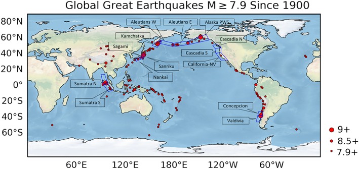
Map with polygons used to define source regions of great earthquakes used in the analysis. Of interest here is the source polygon for the M9.0 Kamchatka earthquake on 4 November 1952. The great earthquakes having M ≥ 7.9 are shown as red circles. These are used to define the histogram of small earthquakes used to compute the earthquake potential score.

We then construct a histogram for the number of small earthquakes between the large earthquakes in the large geographic regions. Focusing next on the local polygon, we count the number of small earthquakes that have occurred since the last large earthquake. Comparing this natural time count (Holliday et al., 2006; Varotsos et al., 2006) to the histogram in the large region determines the earthquake potential score (EPS) from the cumulative distribution function (CDF) constructed from the natural time histogram.

An example of the EPS score is shown in Figure 2 for the Kamchatka source polygon. The M9.0 Kamchatka earthquake occurred in that polygonal source region on 4 November 1952 (www.wsspc.org/resources‐reports/tsunami‐center/significant‐tsunami‐events/1952‐kamchatka‐tsunami/). An associated tsunami generated by the earthquake led to the deaths of 10,000 to 15,000 persons in the Kuril islands (WSSPC [www.wsspc.org/resources‐reports/tsunami‐center/significant‐tsunami‐events/1952‐kamchatka‐tsunami/]). Run‐ups as high as 15 m were observed locally, and run‐ups as large as 1 m were observed as far away as California.

Figure 2.

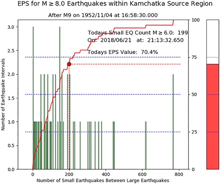
Current earthquake potential score (EPS) for the Kamchatka source polygon. Vertical green bars are the histogram of counts of “small” earthquakes having M ≥ 8.0. The red dot records the current count, 199, of small earthquakes in the polygon, with a corresponding EPS value of 70.4%.

The (green) vertical bars in Figure 2 represent the numbers of 6 ≤ M < 7.9 earthquakes between the M ≥ 7.9 great earthquakes that occurred worldwide since 1950. Small earthquake data from years prior to 1950 are not complete at the M ≥ 6 level (Rundle et al., 2018). The red curve monotonically ascending from lower left to upper right is the CDF corresponding to the histogram. The current count of 199 small earthquakes having magnitudes 6 ≤ M < 7.9 since the great earthquake in 1952 is indicated by the red dot in Figure 2, leading to an EPS value of 70.4%. The interpretation of this statistic is that the Kamchatka source polygon is 70.4% through the typical earthquake cycle characterizing global great earthquakes, as measured by small earthquake counts.

4. Shannon Information Entropy

Shannon information entropy was developed in statistical communication theory as a means to characterize the information content transmitted between a source and a receiver by means of a communication channel (Cover & Thomas, 1991; Shannon, 1948; Stone, 2015). In his 1948 paper, Shannon described a method for computing a metric for the information delivered from a source to a receiver using only binary (yes/no) decisions. Given an “alphabet” of symbols, Shannon showed that the number of decisions needed to send a symbol from the source to the receiver defines the information content of the communication. He related this to the degree of surprise, or “surprisal,” of unanticipated content embedded in the signal.

The typical example is “Alice” sending a dictionary word to “Bob” by means of a binary digital communication device. Alice must send the message letter by letter. So the question is, how many binary digits must Alice send to convey a single letter? If each letter in the alphabet is equally probable (it is not!), the answer is 4.7 bits of information. This value can be determined by the use of equation (1) below, using a letter probability $p_i=\frac{1}{26}$ for the constant probability case.

The principal objective of the present paper is to apply ideas about Shannon information entropy to earthquake physics. Here we use the known earthquake frequency‐magnitude statistics to measure the information that an earthquake is contributing to current hazard calculations.

A reason to believe that information might be contained in earthquake sequences is the idea that earthquakes bear strong similarities to neural networks in terms of the governing equations (Hertz & Hopfield, 1995; Hopfield, 1994; Rundle et al., 2002). It is known that neural networks convey information, and that Shannon information entropy methods are used to characterize their information content (Marzen et al., 2015; Marzen & Crutchfield, 2017).

Neurons are simple elements that emit action potentials or voltage “spikes” in response to driving currents (Hopfield, 1994). Once a neuron fires, typically at a level of −53 mV, the voltage resets to around −70 mV, followed by a refractory period during which the neuron does not fire. The information is contained in the temporal spacing between the spikes (Marzen & Crutchfield, 2017).

On the other hand, earthquakes are caused by tectonic driving forces that lead to a sudden slip event associated with a sudden change in fault stress, a stress “spike.” While neural networks are an electrical system, earthquakes are a mechanical system. The common features of these two systems have been discussed by Hopfield (1994), Hertz and Hopfield (1995), and Rundle et al. (2002). We begin with an analysis of the information contained in the magnitude of the events in earthquake sequences.

To understand information entropy, one starts with an “alphabet” of symbols, each symbol indexed by the integer i. In our case, the “alphabet” will be a sequence of discrete magnitude “bins” centered on a value m _i, each bin being of width Δm. The probability that an earthquake has a magnitude m _i is denoted as p_i.

For a system having discrete states indexed by an integer i, Shannon defined the self‐information I_i as

$$I_i=-{log}_2\left(p_i\right)$$ (1)

(Cover & Thomas, 1991; Shannon, 1948; Stone, 2015).

The equation for average or expectation of Shannon self‐information is

$$I\equiv <I_i>=-{\sum }_i{p}_i{log}_2\left(p_i\right)$$ (2)

It is required that 0 ≤ p_i ≤ 1 and that ∑_ip_i = 1. As a result, I ≥ 0. By construction, I is an expectation or average. As a common practice, we will refer to I as simply the “Shannon information.”

Although we use only earthquake magnitude, the neural network studies suggest that additional information might be found by evaluating the probabilities of earthquake time intervals. In future research, we plan to discuss the similarities and differences between magnitude entropy and interval entropy. Similarly, we might find ways to evaluate entropy of slip‐rate distributions, and other earthquake‐related quantities. A potentially important question might be, is entropy change in one variable correlated with entropy change in another variable? This might imply some sort of crossover information principle important to earthquake predictability.

5. Magnitude Information Entropy

We first examine magnitude information entropy. We start with the Gutenberg‐Richter distribution:

$$N\left(\ge m\right)={10}^{a-\mathit{bm}}$$ (3)

Equation (3) can be interpreted as the survivor distribution for magnitudes m, given the catalog completeness magnitude m _c. The associated CDF P(m|m _c) is then

$$P\left(m|m_c\right)=1-{10}^{b\left(m_c-m\right)}$$ (4)

Using the substitution β ≡ b ln (10), the associated probability density function ρ(m) in magnitude space is found from differentiating (4):

$$\rho \left(m\right)=\beta e^{\beta \left(m_c-m\right)}$$ (5)

For a discrete bin probability centered on a magnitude value m _Δ, the discrete probability density function is

$$p\left(m_{\mathrm{\Delta }}\right)=\varrho \left(m_{\mathrm{\Delta }}\right)\mathrm{\Delta }m=\beta e^{\beta \left(m_c-m_{\mathrm{\Delta }}\right)}\mathrm{\Delta }m$$ (6)

In this case, the “alphabet” of symbols being transmitted is the sequence of magnitude bins beginning at the completeness magnitude m _c, and having width Δm.

We replace the counts of small earthquakes with the sum of the self‐information in magnitude space using equations (1) and (6) (see Rundle et al., 2016). Further, we assume that the coarse‐grained magnitude element is given by the typical magnitude resolution of Δm ≈ 0.1. Thus, we find that the accumulated self‐information I_cum since the last large earthquake is given by combining (1) and (6):

$$I_{\mathit{cum}}=-{\sum }_j\frac{1}{p_j}$$ (7)

where

$$p_j=0.1\beta e^{\beta \left(m_c-m_j\right)}$$ (8)

and index j refers to small earthquakes that have occurred since the last large earthquake.

The result is shown in Figure 3 for the same polygon as in Figure 2, the Kamchatka polygon. Here the EPS is 64.8%, compared to the previous natural time count‐based value of 70.4%.

Figure 3.

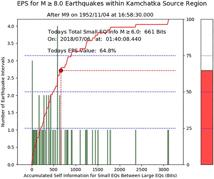
Current earthquake potential score (EPS) for the Kamchatka source polygon. Vertical green bars are the histogram of self‐information in bits for “small” earthquakes having M ≥ 6 between the great earthquakes having M ≥ 8.0. The red dot records the current self‐information value, 661 bits, of small earthquakes in the polygon, with a corresponding EPS value of 64.8%.

Comparing Figures 2 and 3, it can be seen that there is relatively little difference between the values for the EPS. Data for the remainder of the 13 source polygons are shown in Tables 1 and 2. EPS scores shown in Table 1 are based only on natural time counts. In Table 2, the EPS values are based on the sum of self‐information of the small earthquakes since the last great earthquake. Note that small earthquake counts for great earthquakes prior to 1950 are based on estimates whose accuracy is unknown (Rundle et al., 2018), a subject for future research.

Table 1.

Natural Time Nowcast

Location (source)	EPS (%) score	Most recent large EQ	Mag recent large EQ	Count on 2018/06/27	Current M P
Aleutions E	77.8	1946/04/01	8.6	251	8.2
Kamchatka	70.4	1952/11/04	9	199	8.2
Cascadia S	69.4	1922/01/31	7.3	26	7.3
Cascadia N	55.3	1946/06/23	7.5	28	7.4
Calif.‐Nevada	43.0	1906/04/18	7.9	69	7.7
Aleutions W	40.7	1965/02/04	8.7	100	7.9
Alaska PWS	38.9	1964/03/28	9.2	88	7.8
Sagami	25.9	1923/09/01	8.1	64	7.7
Sumatra N	25.9	2004/12/26	9.1	62	7.7
Sanriku	25.9	2011/03/11	9.1	58	7.7
Sumatra S	25.9	2005/03/28	8.6	56	7.6
Valdivia	20.4	1960/05/22	9.5	46	7.6
Concepcion	18.5	2010/02/27	8.8	40	7.5
Nankai	13.0	1946/12/20	8.3	22	7.3

Note. EPS = earthquake potential score.

Table 2.

Information Nowcast

Location (source)	EPS (%) score	Most recent large EQ	Mag recent large EQ	Bits on 2018/06/27	Current M P
Aleutions E	74.1	1946/04/01	8.6	841	8.2
Cascadia S	66.7	1922/01/31	7.3	95	7.3
Kamchatka	64.8	1952/11/04	9	661	8.2
Cascadia N	47.9	1946/06/23	7.5	88	7.4
Calif.‐Nevada	44.3	1906/04/18	7.9	266	7.7
Aleutions W	38.9	1965/02/04	8.7	354	7.9
Alaska PWS	35.2	1964/03/28	9.2	317	7.8
Sagami	24.1	1923/09/01	8.1	216	7.7
Sumatra S	24.1	2005/03/28	8.6	218	7.6
Sumatra N	24.1	2004/12/26	9.1	208	7.7
Sanriku	22.2	2011/03/11	9.1	185	7.7
Valdivia	18.5	1960/05/22	9.5	159	7.6
Concepcion	18.5	2010/02/27	8.8	127	7.5
Nankai	13.0	1946/12/20	8.3	84	7.3

Note. EPS = earthquake potential score.

In some cases, the largest catalog earthquake that occurred in the source polygon is less than M7.9 and is indicated in the 4th column. In other columns we show the date of the most recent great earthquake, its magnitude, the natural time count of M ≥ 6 events since the last great earthquake, and the estimated current potential magnitude M _P of the next great earthquake:

$$M_P=m_c+\left(\frac{1}{b}\right)\mathit{lo}{g}_{10}{n}_s$$ (9)

In equation (9), n _S is the current count of small earthquakes, m _c is the catalog completeness magnitude, and b is the Gutenberg‐Richter b‐value.

Most of the information is contained in the smaller events, primarily because there are so many more of them. This raises the question of whether this method could be modified to more strongly emphasize the larger of the small events. To emphasize this last point, we show in Figure 4 the frequency‐magnitude relation for a region of radius 1,000 km around Tokyo, Japan. In Figure 4a, data are for the time interval from 1 January 1970 through the last event prior to the M9.1 earthquake on 11 March 2011. Figure 4b shows the data following the M7.7 aftershock up to the present.

Figure 4.

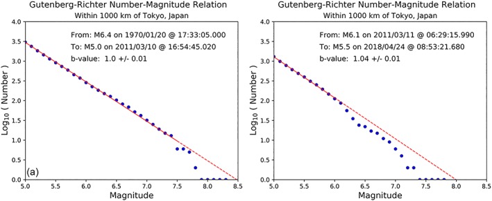
(a) Magnitude‐frequency data for the spatial region within 1,000 km of Tokyo, Japan, prior to the M9.1 mainshock on 11 March 2011. Red solid line indicates the magnitude range fit by the scaling line, from M5.0 to M7.5. (b) Magnitude‐frequency data for the spatial region within 1,000 km of Tokyo, Japan, following the M7.7 aftershock on 11 March 2011. Red solid line indicates the magnitude range fit by the scaling line, from M5.0 to M6.0.

Figure 4a shows that the data are well fit at almost all magnitude intervals by a Gutenberg‐Richter scaling line having a slope, or b‐value of 1.0 ± 0.1. This can be considered to be the long‐term average behavior of earthquakes in the region. On the other hand, the data in Figure 4b show that the scaling line is first re‐established at the small magnitude end, and that there is a deficiency of larger magnitude earthquakes relative to the scaling line. The b‐value of the scaling line in Figure 4b is 1.04 ± 0.1, nearly the same as in Figure 4a. This deficit in larger earthquakes is eventually removed as larger earthquakes occur.

6. Summary and Conclusions

This paper has focused on a first study to incorporate measures of Shannon information entropy into the nowcasting method. A question that has been addressed elsewhere is the issue of the sensitivity of the EPS values to the data used to define the histogram and therefore the CDF.

We have shown in companion papers (Rundle et al., 2018) that the nowcasting method is generally not very sensitive to the choice of large spatial region defining the histogram, leading to a standard error of approximately ±10%. However, the method is strongly sensitive to issues of catalog completeness (Rundle et al., 2018).

Extending our current results to great earthquakes that occurred prior to 1950, the beginning of catalog completeness for magnitudes M ≥ 6, is at this time only approximate. To rectify this problem, we will require additional assumptions, such as estimates of aftershock activity, together with estimates of magnitude statistics.

We have found that in this first study, the results of using magnitude information are similar to those found using only natural time counts of events. The primary reason for this is that even though large magnitude events carry more information than small magnitude events, there are many more small magnitude events at approximately the catalog completeness magnitude. Thus the information entropy at these small events dominates the total self‐information sum.

Further work will investigate techniques to focus attention on primarily the largest events. In future work we also plan to incorporate temporal information in the Shannon information measures through the use of methods similar to those developed in connection with models for Epidemic Type Aftershock Sequences and their derivative methods such as the Branching Aftershock Sequence Statistics (Helmstetter & Sornette, 2003; Ogata, 2004; Turcotte et al., 2007).

Data Sources

The data used in this paper were downloaded from the online earthquake catalogs maintained by the U.S. Geological Survey (https://earthquake.usgs.gov/earthquakes/search/), accessed between June through August, 2018.

Rundle, J. B. , Giguere, A. , Turcotte, D. L. , Crutchfield, J. P. , & Donnellan, A. (2019). Global seismic nowcasting with Shannon information entropy. Earth and Space Science, 6, 191–197. 10.1029/2018EA000464

References

- Cover, T. M. , & Thomas, J. A. (1991). Elements of information theory. John Wiley, NY. ISBN 0–471–06259‐6 [Google Scholar]
- Gomberg, J. , Beeler, N. M. , Blanpied, M. , & Bodin, P. (1998). Earthquake triggering by transient and static deformations. Journal of Geophysical Research, 103, 24,411–24,426. 10.1029/98JB01125 [DOI] [Google Scholar]
- Helmstetter, A. , & Sornette, D. (2003). Predictability in the epidemic‐type aftershock sequence model of interacting triggered seismicity. Journal of Geophysical Research, 108(B10), 2482 10.1029/2003JB002485 [DOI] [Google Scholar]
- Hertz, A. V. M. , & Hopfield, J. J. (1995). Physical Review Letters, 75, 1222–1225. 10.1103/PhysRevLett.75.1222 [DOI] [PubMed] [Google Scholar]
- Hill, D. P. , & Prejean, S. G. (2007). Dynamic triggering In Schubert G. & Kanamori H. (Eds.), Earthquake seismology, Treatise on Geophysics, Schubert, G (Editor‐In Chief) (Vol. 4, pp. 257–291). Amsterdam: Elsevier. [Google Scholar]
- Holliday, J. R. , Graves, W. R. , Rundle, J. B. , & Turcotte, D. L. (2016). Computing earthquake probabilities on global scales. Pure and Applied Geophysics, 173, 739–748. 10.1007/s00024-014-0951-3 [DOI] [Google Scholar]
- Holliday, J. R. , Rundle, J. B. , Turcotte, D. L. , Klein, W. , Tiampo, K. F. , & Donnellan, A. (2006). Using earthquake intensities to forecast earthquake occurrence times. Physical Review Letters, 97, 238,501. [DOI] [PubMed] [Google Scholar]
- Hopfield, J. J. (1994). Neurons, dynamics and computation. Physics Today, 47, 40–46. 10.1063/1.881412 [DOI] [Google Scholar]
- Jolliffe, I. T. , & Stephenson, D. B. (2003). Forecast Verification, A Practitioner's Guide in Atmospheric Science. NJ, USA: Wiley. [Google Scholar]
- Kelleher, J. A. , Sykes, L. R. , & Oliver, J. (1973). Possible criteria for predicting earthquake locations and their applications to major plate boundaries of the Pacific and Caribbean. Journal of Geophysical Research, 78, 2547–2585. 10.1029/JB078i014p02547 [DOI] [Google Scholar]
- Marshall, J. L. , Jung, J. , Derber, J. , Chahine, M. , Treadon, R. , Lord, S. J. , Goldberg, M. , Wolf, W. , Liu, H. C. , Joiner, J. , Woollen, J. , Todling, R. , vab Delst, P. , & Tahara, Y. (2006). Improving global forecasting and analysis with AIRS. Bulletin of the American Meteorological Society, 87, 891–894. [Google Scholar]
- Marzen, S. E. , & Crutchfield, J. P. (2017). Structure and randomness of continuous‐time, discrete‐event processes. Journal of Statistical Physics, 169, 303–315. 10.1007/s10955-017-1859-y [DOI] [Google Scholar]
- Marzen, S. E. , DeWeese, M. R. , and Crutchfield, J. P. (2015), Time resolution dependence of information measures for spiking neurons: Atoms, scaling, and universality, Santa Fe Institute Working Paper. arXiv:1504.04756v1[q‐bio.NC] 18 April (2015) [DOI] [PMC free article] [PubMed]
- Nishenko, S. P. (1991). Circum‐Pacific seismic potential—1989–1999. Pure and Applied Geophysics, 135, 169–259. [Google Scholar]
- Ogata, Y. (2004). Space‐time model for regional seismicity and detection of crustal stress changes. Journal of Geophysical Research, 109, B03308 10.1029/2003JB002621 [DOI] [Google Scholar]
- Rogerson, P. A. (2018). Statistical evidence for long‐range space‐time relationships between large earthquakes. Journal of Seismology, 30 10.1007/s10950-018-9775-4 [DOI] [Google Scholar]
- Rundle, J. B. , Luginbuhl, M. , Giguere, A. , & Turcotte, D. L. (2018). Natural time, nowcasting, and the physics of earthquakes: Estimation of seismic risk to global megacities. Pure and Applied Geophysics, 175, 647–660. 10.1007/s00024-017-1720-x [DOI] [Google Scholar]
- Rundle, J. B. , Tiampo, K. F. , Klein, W. , & Martins, J. S. S. (2002). Self‐organization in leaky threshold systems: The influence of near mean field dynamics and its implications for earthquakes, neurobiology and forecasting. Proceedings of the National Academy of Sciences of the United States of America, 99(Supplement 1), 2514–2521. [DOI] [PMC free article] [PubMed] [Google Scholar]
- Rundle, J. B. , Turcotte, D. L. , Donnellan, A. , Grant‐Ludwig, L. , & Gong, G. (2016). Nowcasting earthquakes. Earth and Space Science, 3, 480–486. [Google Scholar]
- Sarlis, N. V. , Skordas, E. S. , & Varotsos, P. A. (2011). The change of the entropy in natural time under time‐reversal in the Olami–Feder–Christensen earthquake model. Tectonophysics, 513(1), 49–53. [Google Scholar]
- Sarlis, N. V. , Skordas, E. S. , Varotsos, P. A. , Ramírez‐Rojas, A. , & Flores‐Márquez, E. L. (2018). Natural time analysis: On the deadly Mexico M8.2 earthquake on 7 September 2017. Physica A, 506, 625–634. [Google Scholar]
- Savage, H. M. , & Marone, C. (2008). Potential for earthquake triggering from transient deformations. Journal of Geophysical Research, 113, B05302 10.1029/2007JB005277 [DOI] [Google Scholar]
- Scholz, C. H. (2002). The mechanics of earthquakes and faulting (2nd ed.p. 471). New York: Cambridge Univ. Press. [Google Scholar]
- Shannon, C. E. (1948). A Mathematical Theory of Communication. Bell System Technical Journal, 27, 379–423 & 623–656, July & October. [Google Scholar]
- Stone, J. V. (2015). Information theory: A tutorial introduction. Sheffield, UK: Sebtel Press. ISBN978–0–9563728‐5‐7 [Google Scholar]
- Turcotte, D. L. , Holliday, J. R. , & Rundle, J. (2007). BASS, an alternative to ETAS. Geophysical Research Letters, 34, L12303 10.1029/2007GL029696 [DOI] [Google Scholar]
- Vallianatos, F. , Michas, G. , Papadakis, G. , & Sammonds, P. (2012). A nonextensive statistical physics view to the spatiotemporal properties of the June 1995, Aegean earthquake (M6. 2) aftershock sequence (West Corinth rift, Greece). Acta Geophysica, 60(3), 758–768. [Google Scholar]
- Varotsos, P. A. , Sarlis, N. V. , Efthimios S Skordas, E. S. , & Tanaka, H. (2004). A plausible explanation of the b‐value in the Gutenberg‐Richter law from first principles. Proc. of the Japan Acad. Series B, 80(9), 429–434. [Google Scholar]
- Varotsos, P. A. , Sarlis, N. V. , Skordas, E. S. , Tanaka, H. K. , & Lazaridou, M. S. (2006). Attempt to distinguish long‐range temporal correlations from the statistics of the increments by natural time analysis. Physical Review E, 74, 021123. [DOI] [PubMed] [Google Scholar]
- Varotsos, P. A. , Sarlis, N. V. , Tanaka, H. K. , & Skordas, E. S. (2005). Similarity of fluctuations in correlated systems: The case of seismicity. Physical Review E, 72, 041103 10.1103/PhysRevE.72.041103 [DOI] [PubMed] [Google Scholar]