Abstract
We propose a new algorithm, called line integral alternating minimization (LIAM), for dual-energy X-ray CT image reconstruction. Instead of obtaining component images by minimizing the discrepancy between the data and the mean estimates, LIAM allows for a tunable discrepancy between the basis material projections and the basis sinograms. A parameter is introduced that controls the size of this discrepancy, and with this parameter the new algorithm can continuously go from a two-step approach to the joint estimation approach. LIAM alternates between iteratively updating the line integrals of the component images and reconstruction of the component images using an image iterative deblurring algorithm. An edge-preserving penalty function can be incorporated in the iterative deblurring step to decrease the roughness in component images. Images from both simulated and experimentally acquired sinograms from a clinical scanner were reconstructed by LIAM while varying the regularization parameters to identify good choices. The results from the dual-energy alternating minimization algorithm applied to the same data were used for comparison. Using a small fraction of the computation time of dual-energy alternating minimization, LIAM achieves better accuracy of the component images in the presence of Poisson noise for simulated data reconstruction and achieves the same level of accuracy for real data reconstruction.
Keywords: line integral, dual-energy, X-ray CT, alternating minimization algorithm, iterative deblurring algorithm
I. Introduction
An important quantitative application of X-ray computed tomography (CT) is the imaging of radiological properties of the underlying tissues. For example, use of quantitative single-energy CT imaging [1],[2] to determine relative electron density on a voxel-by-voxel basis is standard-of-practice in mega-voltage radiation therapy planning. However, single-energy CT imaging is inadequate for high-energy charged particle beams and low energy (<100 keV) photon fields, because their interactions with tissue are sensitive to both tissue composition and electron density.
In proton beam therapy, state-of-the-art single-energy CT imaging results in residual stopping power-ratio measurement uncertainties [3] that lead not only to dose-computation errors, but to geometric targeting errors (called “range uncertainty” errors): 3–7 mm uncertainties in the depth of the sharp distal falloff of the spread-out Bragg peak.
The transport and absorption of low energy (<100 keV) X-ray photons in tissue is highly sensitive to both electron density and tissue composition, because photoelectric absorption varies with the cube of the atomic number of the tissue (Z). Because conventional single-energy 70 keV clinical CT imaging cannot distinguish between density and effective atomic number changes, patient-specific photon cross section is generally not available for medical applications requiring radiation transport calculations. Tissue-specific atomic composition measurements are very sparse and demonstrate large sample-to-sample variations. Hence the standard ICRP [4] tissue compositions have heretofore potentially large uncharacterized uncertainties. One application where patient dosimetry is hindered by these circumstances is low energy interstitial seed brachytherapy. In this energy range (20–35 keV) neglecting tissue composition heterogeneities introduces large (10%–50%) systematic errors into dose computation [5]. Patient-specific estimation of organ doses from diagnostic CT imaging [6] is another application that is hindered by lack of quantifiably accurate photon cross sections. Finally, the full clinical benefits of iterative model-based CT image reconstruction techniques can only be realized with accurate a priori knowledge of elemental composition of the underlying tissues. This is necessary because of the limited effectiveness of water-equivalent beam-hardening preprocessing and data linearization corrections.
Quantitative dual-energy CT stands as an attractive modality to address the problem of in-vivo determination of tissue radiological properties. The use of different energies allows for the estimation of photon cross sections and proton stopping powers, which requires at least two independent measurements at different energies [7],[8]. In addition, CT image intensities approximate linear attenuation coefficients.
Modeling studies have demonstrated that low-energy photon cross sections can be modeled with acceptable accuracy (1%–3% in the 20–1000 keV energy range) utilizing either effective electron density and [7],[9] or a linear combination of two dissimilar materials [8] as surrogates for elemental tissue composition and density.
Unfortunately, photon cross-section imaging via dual energy CT imaging is a physically challenging measurement since small differences in high-to-low energy tissue contrast correspond to very large changes in photoelectric cross section. In their simulation of post-processing dual-energy analysis, Williamson et al. [8] demonstrated that systematic and random uncertainties in image intensity must to be limited to 0.2%–0.5% in order to recover linear attenuation coefficients with an uncertainty less than 3%. This specification cannot be achieved by commercial scanners using filtered back projection at clinically feasible doses and resolutions. However, our group [10] has experimentally demonstrated that photon cross sections can be measured on a clinical scanner with an accuracy better than 1% provided that image artifacts and noise can be eliminated.
Model-based iterative algorithms[11], [12], [13], [14], [15], [16] seek to identify optimal images which maximize fidelity to the measured projection data. These algorithms are attractive because systematic artifacts, (such as those due to beam hardening, scatter, image blur, and incompletely sampled projections) can be minimized using physically realistic signal formation models [17],[18]. In particular, regularized statistical image reconstruction algorithms, which model the statistics of signal formation, provide a 2- to 5-fold more favorable tradeoff between spatial resolution and signal-to-noise ratio than filtered back projection [19].
In our previous work, the use of a statistical image reconstruction algorithm [20] reduced cross section measurement uncertainty two fold [10],[21]. The most prevalent algorithm in spectral CT including dual-energy CT corresponds to the basis material decomposition (BMD) algorithm proposed by Alvarez and Macovski in 1976 [22]. The BMD algorithm assumes the linear attenuation coefficient μ(x, E) of the scanned object are expressed as a linear combination of some basis functions,
where f1, f2, …, fi, …, fI are the linearly independent basis material attenuation functions and c1, c2, …, ci, …, cI are the corresponding coefficients.
Many possible choices of basis functions have been proposed, including a two component (I = 2) basis pair originally recommended by Alvarez and Macovski, consisting of approximations to the photoelectric absorption and scattering cross sections. In this study, we utilize a basis pair consisting of two dissimilar reference materials that bracket the range of biological media contained in typical patients:
A study by Williamson et al. [8] demonstrates that this model is able to parameterize linear attenuation coefficients and mass energy absorption coefficients, along with scattering and photoelectric effect cross sections, with 1–2% accuracy in the 20 keV to 1 MeV energy range.
Dual energy reconstruction methods in the literature typically fall into one of three classes. The first method is the post-processing class [8], in which images from each scan are computed separately, then combined afterwards to compute component image estimates. Mathematically, the coefficients c1(x) and c2(x) are expressed as the product of a 2 by 2 matrix T (T = K−1, Ki,j = ∫E Sj(E)fi(E)dE) and two sets of input image data corresponding to two spectra. The input image data are expressed as ∫E Sj(E)μ(x, E)dE, where Sj(E) is the normalized spectrum with ∫E Sj(E)dE = 1 and j indexes the spectrum. The second method is the preprocessing class [22],[23],[24], in which the scan sinograms are combined to extract estimates of scans of single components/ basis from which the single component/base image estimates are recovered through image reconstruction. In preprocessing methods, the basis material model replaces the linear attenuation coefficients in the mathematical expressions of measurements which are governed by Beer’s law. Then the line integrals of the coefficients c1(x) and c2(x) can be computed based on the measurements. Finally, the coefficients c1(x) and c2(x) can be calculated. The third method is the joint-processing class, in which the dual-energy scan data are processed simultaneously to directly recover component image estimates. Fessler et al. [25] found a paraboloidal surrogate function for the original log-likelihood function [15]. Zhang et al. [26] used a quadratic approximation of the negative log-likelihood function[16]. The approaches presented in this work correspond to the joint-processing class, as do any statistical image reconstruction algorithms based on a direct comparison of the raw measurements to mean data predicted from the component images.
There are, however, some ambiguities in the classification above. Linear operations on attenuation data that have been pre-corrected for beam-hardening may commute with linear reconstruction. An exception is the pair of two-component models used by Williamson et al. [8], with the components selected in the post-processing stage based on the values of the linear attenuation coefficients in the reconstructed images.
There are also limitations to single component/base reconstructions followed by post-processing of the result. The errors in the single component/base model can be significant, and can be amplified in the resulting post-processing. Similarly, preprocessing can amplify noise in the individual scans, yielding significant errors in the resulting images. The pre-processing methods can be very sensitive to the deviation between the choice of basis functions and the true composition of the object. A mismatch between them can cause systematic errors as well as image artifacts such as streaking [27]. Moreover, since the pre-processing method neglects noise characteristics, it can produce very noisy estimates in the low dose scenario. To reduce the noise in the estimates, Noh et al. [28] proposed to use penalized weighted least squares and penalized likelihood methods based on statistical models. By incorporating two components in the forward model and directly comparing the measured data to the predicted mean data using a data log-likelihood function, joint-processing methods quantitatively account better for the underlying physics than post and preprocessing methods.
O’Sullivan and Benac developed an alternating minimization (AM) algorithm [20],[29] for a polyenergetic CT data model. Their approach is to find the maximum likelihood estimates of the two component images within a Poisson data model framework. This method is based on the fact that maximizing log-likelihood is equivalent to minimizing I - divergence [30]. They extended this AM algorithm to a dualenergy alternating minimization (DE-AM) algorithm, in which a regularizer can be incorporated to improve image smoothness [31]. While regularized DE-AM algorithms can produce quantitatively accurate component images, these methods suffer from slow convergence. Even with the ordered subset (OS) technique, over 2000 iterations are required for convergence, according to our implementation. Jang et al. [32] proposed a very similar approach called information-theoretic discrepancy based on iterative reconstructions (IDIR); they compared AM to IDIR and showed slow convergence. One reason for the slow convergence is that the two component attenuation functions are highly correlated, leading to high correlation in the estimates of the corresponding images.
This ill-conditioned problem formulation poses challenges for all statistical image reconstruction algorithms. Reducing this correlation might speed up the convergence. An extensive study of the effect of the correlation can be found in [33].
A. LIAM in Relation to Literature
Our optimization approach is motivated by first reformulating the original image reconstruction problem (as cast in [31]) as a constrained optimization problem, then softening the constraint by not forcing equality. This is analogous to a variable splitting approach [34] in that additional variables are introduced separating the data fit term from the constraint.
The line integral alternating minimization (LIAM) algorithm alternates between the evaluation of the line integrals (optimization in data space, analogous to pre-processing) and the images (optimization in image space). In LIAM, the high correlation between components remains in the estimates of the two line integrals from the dual energy measurements, but not in the individual voxel estimates. While this may lead to large errors in the estimated line integral values, these are smoothed by the second term that penalizes the discrepancy between the line integrals and the forward-projected images. These predicted sinograms are smooth, introducing smoothing to the estimated line integrals.
The algorithm described here is easily extended to more than two measurement spectra and attenuation components, so it is directly applicable to a broad array of spectral CT problems. Our emphasis on dual energy is due to its availability in clinical scanners.
There is an alternative interpretation of the soft constraint between line integrals determined from the data and line integrals predicted from estimated component images. The forward model from image space to line integrals is approximate, so the soft constraint can be interpreted as making the algorithm robust to errors in the forward model.
There are many approaches in the literature for variable splitting including the related split Bregman [35], method of multipliers [36], and alternating direction method of multipliers (ADMM) [37]. While motivated by these approaches, our algorithm avoids the use of square error preferring I-divergence. I-divergence is an information-theoretic measure that results from an axiomatic derivation of discrepancy over nonnegative vectors [38], [39]. As described by Boyd et al. [37], a goal of ADMM is the same as ours, namely to decompose the problem into a set of smaller problems, each such smaller problem being solvable.
ADMM has been successfully applied to X-ray CT imaging [40], [41]; Tracey and Miller [42] derive an algorithm using ADMM with a total variation penalty combined with nonlocal means. Sawatsky et al. [43] use a version of ADMM along with a sparsity-promoting penalty for spectral CT. Wang and Banerjee [44] introduce a generalization of ADMM by allowing an arbitrary Bregman divergence to be substituted in place of the square difference used in ADMM; we use I-divergence which is a Bregman divergence. Our algorithm uses an I-divergence surrogate for the data fit term and is thus not a Bregman ADMM algorithm.
The rest of the paper is organized as follows. We first introduce the data model, the problem definition, as well as the algorithm in Section II. Section III sketches regularized LIAM algorithm, which uses an edge-preserving penalty function. Sections IV and V provide reconstructions with different regularization parameters for simulated data and real data from the Philips Brilliance Big Bore scanner (Philips Healthcare, Cleveland, Ohio), respectively.
II. LIAM Algorithm
We propose to minimize I -divergence between the data and the estimated mean represented by line integrals L (vector with dimension equal to the number of measurements), subject to a soft projection constraint on the discrepancy between Li and Hci, where ci is the component image (vector with dimension equal to the number of pixels) with i indexing the component and H = h(y, x) (matrix with row size equal to the number of measurements and column size equal to the number of pixels) is the discrete approximation to the projections that links the component image and the line integral. Essentially, we seek the maximum likelihood estimates of the line integrals subject to the soft projection constraint, and eventually, when the constraint is satisfied with equality, we actually obtain the maximum likelihood estimates of the component images. The soft projection constraint is introduced as the I -divergence between the line integral and forward projection of the image, with a Lagrange multiplier. Then by alternately updating L and c while keeping the other fixed, we can obtain converged line integrals and images. We update integrals by using Newton’s method and update images by using an iterative deblurring (ID) algorithm [45]. If necessary, we can add a neighborhood penalty when updating images by using a trust region Newton’s method (regularized ID algorithm).
A. Data Model
Denote the source-detector measurement pairs by y, pixels by x and X-ray spectra by j ∈ {1, 2}. The X-ray spectra I0j(y, E), j = 1, 2 depend on energy indexed by E and typically depend on the source-detector pair (for example, due to a bow-tie filter). E denotes discretized energy level (for our implementations, the increment for values of E is 1 keV, the minimum energy is 10 keV and the maximum energy is determined by the kVp of the source spectrum). The transmission data dj(y) are assumed to be Poisson distributed with means Qj [c1, c2](y),
| (1) |
where ci(x), i = 1, 2 are the component images [20], with nonnegativity constraint, μi(E) represents the attenuation of a basis material, and I0j represents the number of unattenuated photons absorbed by the detector. The explicit dependence of Qj on [c1, c2] may be dropped if it is clear from context.
All models for transmission data are approximate and limited. The assumption of Poisson data is appropriate for photon-counting (including energy-sensitive photon-counting) detectors. The detectors in typical clinical scanners are energy-integrating, resulting in a compound Poisson process model for which a modified Poisson model is an approximation [46], [47], [48]. Other authors use weighted Gaussian distribution models for the data.
B. Problem Definitions
We use I -divergence to measure the discrepancy between the measured data and the estimated mean. The original image reconstruction problem [31] is
| (2) |
We reformulate (2) as a constrained optimization problem
| (3) |
where
| (4) |
i.e. Fj(y) is directly a function of Li(y) not ci(x); however, with the constraint that Li(y) = ∑xh(y, x)ci(x), i ∈ {1, 2}, (3) and (2) become identical.
As has been shown by Chen [33], the original algorithm has slow convergence, therefore, we want to soften the constraint by not forcing equality of the constraint (i.e., Li(y) = ∑xh(y, x)ci(x), i ∈ {1, 2}). Using I-divergence as a discrepancy, the new optimization problem is min
| (5) |
where
| (6) |
where the term multiplying β penalizes the differences between the estimated line integrals and the forward projections of the component images and β is the parameter that controls the tradeoff between the data fit term and the penalty term. In the extreme case when β → +∞, the penalty term must go to zero, and (5) becomes equivalent to the original problem in (3) and (2).
C. Reformulation of Problem
The Convex Decomposition Lemma [20] provides a variational representation for the data fit term in our problem. That is, the data fit or log-likelihood term can be written as the result of minimizing over auxiliary variables
| (7) |
where fj(y, E) takes values in the exponential family of nonnegative functions parameterized by Li, i = 1, 2,
| (8) |
pj takes values in the linear family of distributions determined by the data
| (9) |
(we refer to “family” as a set of probability distributions of a certain form), and the I-divergence on the right side includes sums over source-detector pairs y and energies E,
| (10) |
We can then reformulate our problem as min
| (11) |
Updating Li, i = 1, 2 is equivalent to updating fj, j = 1, 2 since fj lies in the exponential family parameterized by Li.
D. Alternating Minimization Iterations
There are three steps in every iteration of which the pj and ci updates are easy.
The updating step for pj is analogous to the updating step described for DE-AM, which is
| (12) |
The updating step for ci is the same as the ID algorithm update [45], which is
| (13) |
Note that here k indexes the main iteration regarding updating pj, fj and ci, and n indexes the iteration inside the ID algorithm to recover ci alone, for fixed pj and fj.
In terms of updating fj or Li, we use Newton’s method, since the problem is strictly convex and one extra use of the convex decomposition lemma from DE-AM algorithm can be avoided. The gradient for (L1(y), L2(y))T is ∇(y) = (∇1(y), ∇2(y))T, where
| (14) |
The corresponding Hessian matrix is , where
| (15) |
The pseudocode for LIAM algorithm is as follows:
|
Note that in the procedure, the choice of β is not discussed. It can be held fixed or incrementally changed during iterations using a fixed schedule. One motivation for using a dynamic selection for β during iterations is that using β → 0 can empirically promote convergence which is desirable at early iterations, then as iterations proceed, a larger β will enforce the projection constraints more, forcing the line integrals to lie in the range space of h(y, x).
III. Regularized LIAM Algorithm
As with the DE-AM algorithm, desirable smooth images can be achieved using regularization. In the setup of LIAM algorithm, we cannot apply regularization to the estimated line integrals directly since the smoothness prior does not pertain to the line integrals. Instead, we need to apply regularization to the ID algorithm which recovers the component images.
The regularization form we used is
| (16) |
where φ is the selected potential function; 𝒩x is the neighborhood pixels surrounding pixel x. The weights wx,k control the relative contribution of each neighbor. In all the reconstructions in this paper, 𝒩x is the 8-pixel neighborhood surrounding pixel x and wx,k are set to be the inverse distance between pixel centers.
We use a type of edge-preserving potential function
| (17) |
which has been used by many researchers [49],[50],[51]. In this potential function, t is the intensity difference between neighboring pixels/voxels, δ is a parameter that controls the transition (cutoff point is at 1/δ) between a quadratic region (for small t) and a linear region (for larger t) and we will explore later the effects of δ on the reconstructed images.
The total objective function we are trying to minimize is
| (18) |
where λ is a scalar that reflects the amount of smoothness desired for fixed β, and βλ controls the tradeoff between data fit (I -divergence) and image smoothness (regularization). In the implementation of this paper, a single λ value controls the smoothness constraint for both component images. More λ’s can be incorporated to have independent control over each component.
We use a convex decomposition of the penalty as introduced by De Pierro [52], and the resulting objective function (18) is strictly convex and a trust region Newton’s method [53] can be applied to solve for the component images. Therefore, regularized LIAM algorithm differs from unregularized LIAM only in the ID step (step D in the pseudocode of unregularized LIAM) which solves for the component images, where we use the trust region Newton’s method to incorporate the penalty rather than a regular ID update step.
After the update for (step C in the pseudocode of unregularized LIAM), the decoupled objective function for every is,
| (19) |
where . The pseudocode for the trust region Newton’s method in regularized LIAM is as in Appendix.
In the implementation of regularized LIAM, β and λ can be selected jointly to achieve the desired image quality. When β approaches zero, the terms with βλ as weighting in the front are negligible, and the updates of the line integrals do not depend on the reconstructed images. In the following reconstructions, β → 0 corresponds to the limiting case as β approaches zeros, therefore, the updating becomes a simple two-step procedure: after the line integrals are updated, by using some value of λ, the component images can be recovered.
In summary, we use “unregularized/regularized LIAM algorithm” to specify whether a neighborhood penalty function is used. β → 0 corresponds to the case that the estimation of line integrals and component images are decoupled, and a simple two step algorithm is applied: updating the line integrals without considering the component images for k iterations, then at kth iteration, updating component images using the ID algorithm or the trust region Newton’s method with nonnegativity constraint for some iterations based on the estimated line integrals. β ≠ 0 corresponds to the case that the estimation of line integrals is coupled with the estimation of component images and step C in the pseudocode is applied to solve for the line integrals.
IV. Simulation Results and Discussions
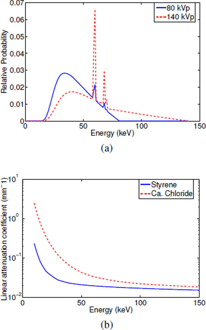
In this section, the simulated image size is 64 × 64 with pixel size 1 mm × 1 mm. The initial conditions are uniform images with pixel intensities equal 1. I0 = 100000, which corresponds to the mean number of unattenuated photons per detector. The two component materials used are polystyrene (c1(x)) and calcium chloride solution (c2(x)), which is a mixture of 23% calcium chloride and 77% water by mass. The attenuation coefficient spectra for the two components are shown in Fig. 1b.
Fig. 1.
(a) Incident spectra computed using Xcomp5 [54] and (b) Attenuation coefficients of the component materials for simulated data reconstruction.
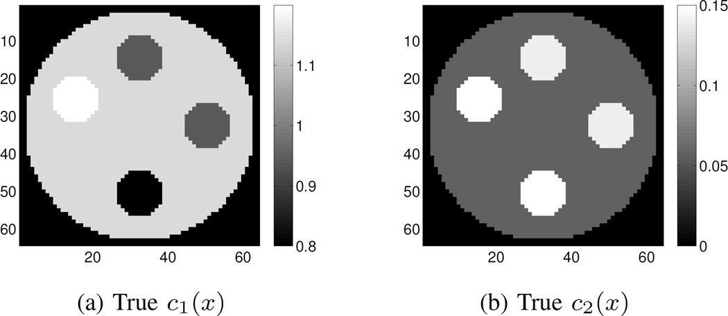
A mini CT scanner geometry is used for generating simulated data consisting of 360 source angles and 92 detectors in the detector fan. Fig. 1a shows the two incident energy spectra corresponding to tube voltages of 80 kVp and 140 kVp. The phantom consists of a cylindrical polymethylmethrylate (PMMA) core in air. The core has four openings for housing different materials. We simulate samples of muscle, teflon and cortical bone substitute with the two component materials (polystyrene and calcium chloride solution) in the proportions listed in Table I. The true component images for polystyrene (c1(x)) and calcium chloride solution (c2(x)) are shown in Fig. 2.
TABLE I.
Component coefficients of the phantom for mini CT geometry.
| Substance | Polystyrene | Calcium Chloride Solution |
|---|---|---|
| Muscle | 0.940 | 0.139 |
| Teflon | 1.42 | 0.488 |
| Cortical Bone Substitute | 0.030 | 2.86 |
| PMMA | 1.14 | 0.0583 |
Fig. 2.
Simulated phantom. (a) True polystyrene (c1(x)) image; (b) True calcium chloride solution (c2(x)) image. Starting from 12 o’clock, clockwise, the inserted rods are muscle, muscle, cortical bone and teflon. The background core is made of PMMA.
The computation platform used in the experiments of this paper is with Intel Core i7-3960X CPU at 3.3-GHz. 64GB of RAM is installed along with 64-bit Windows 7 operating system.
A. Reconstruction with β → 0 and Fixed λ
LIAM reconstructions were first explored with β → 0 corresponding to the case when the penalty term is negligible compared to data fit term, so the updates for line integrals do not depend on reconstructed images for all iterations. As a result, the ID image reconstruction step was performed only after the convergence of the line integral estimates. However, for the purpose of evaluating the I -divergence in (2), we still cycle through step B to D for every iteration, even though step D does not give feedback to step B and C.
We first test the unregularized (corresponding to λ = 0) version of LIAM algorithm with β → 0. We compare the 100 iterations reconstruction results of unregularized LIAM and the 36700 iterations reconstruction results of unregularized DE-AM without OS, using noiseless data. For the Poisson noisy data, the 100 full iterations reconstruction results of unregularized LIAM and the 22500 iterations reconstruction results of unregularized DE-AM without OS were used. The reason for choosing the reconstructions corresponding to a certain number of iterations is that if we compare the I - divergence terms that are the data fit terms inside the objective function, the two results have similar I -divergence values. Due to limited iterations, neither the unregularized LIAM algorithm nor the unregularized DE-AM algorithm gives perfect reconstructions using noiseless data. In general, the unregularized LIAM algorithm achieves more accurate mean estimation compared to unregularized DE-AM algorithm. In particular, for cortical bone substitute, the unregularized DEAM algorithm gives significant overestimation in c1(x) and underestimation in c2(x). However, unregularized LIAM has almost ten times larger standard deviations when noise is present compared to noiseless data, while unregularized DEAM gives similar standard deviations as well as means, for noiseless and noisy data. Unregularized LIAM seems very sensitive to noise, hence regularization is needed.
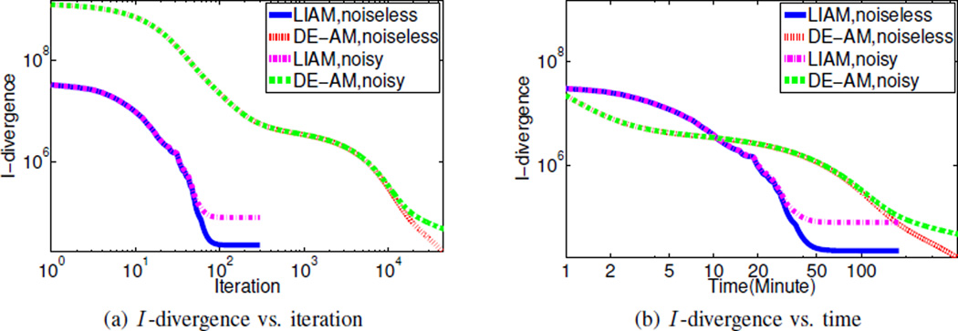
We can also plot the evolution of I -divergence (between the data and the mean represented by the reconstructed images) in order to compare the convergence of unregularized LIAM algorithm to unregularized DE-AM algorithm, as seen in Fig. 3. We see that unregularized LIAM algorithm converges much faster than unregularized DE-AM algorithm for both noiseless data and noisy data, in terms of both iteration and time. While this is not a fair comparison since the I -divergence in unregularized LIAM algorithm is computed in terms of component images, which is not the objective function LIAM algorithm tries to minimize, Fig. 3 does show a much faster convergence. Also, it takes about 100 iterations or 50 minutes for unregularized LIAM algorithm to converge, but compared to the noiseless data reconstruction, the noisy data reconstruction converges to a higher I -divergence, and this I -divergence value is about the same order as the I -divergence between the noisy data and the mean data. Moreover, for unregularized LIAM algorithm (when β → 0), since updating line integrals does not depend on the update of images, the running time of unregularized LIAM can be reduced significantly.
Fig. 3.
(a) I -divergence vs. iteration and (b) I -divergence vs. time using unregularized LIAM algorithm with β → 0 and unregularized DE-AM algorithm for simulated data reconstruction. I -divergence is evaluated according to (2).
B. Reconstruction with Dynamic β and λ
The introduction of β and λ in the LIAM algorithm offers flexibility to control the reconstruction performance as well as the convergence rate. However, at the same time, it adds complexity in terms of choosing the correct parameters. We try to explore the parameter space to achieve the best image smoothness while maintaining high estimation accuracy.
From the previous section, we can see that by running unregularized LIAM with β → 0, the reconstructed images can achieve high mean estimation accuracy, but are very noisy. In order to improve image smoothness, we will use nonzero β to incorporate the projection constraint, as well as image smoothness regularization to directly add a neighborhood penalty. We compare the reconstruction results of regularized LIAM after 200 full iterations (updating pj, Li and ci) with different λ values, using the same Poisson noisy data as before. Note that in the reconstructions, we set β → 0 for the first 100 iterations and β = 1000 for the second 100 iterations. For the first 100 iterations, the (unregularized) ID algorithm is used for reconstructing images while for the second 100 iterations, a trust region Newton’s method is used.
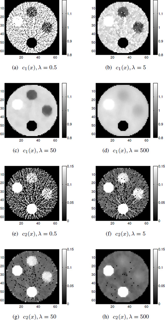
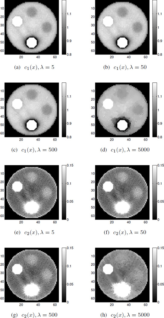
According to the results shown in Fig. 4, λ = 0.5 and λ = 5 do not give a strong enough neighborhood penalty while λ = 500 is too strong and washes out some regions, causing mean intensity changes which sacrifice accuracy. Among these λ choices, λ = 50 performs best, even though there are isolated speckles for c2(x). The“speckles” are just noisy pixels in which the intensity is below the chosen window level values and these stick out as very noticeable black pixels. It is worth mentioning that the choice of β and λ should be considered jointly, since according to (18), the neighborhood penalty weight is βλ in the overall objective function. Reconstructions of 25000 iterations using regularized DE-AM without OS are also presented in Fig. 5 for comparison, with δ = 500, λ = 5, 50, 500, 5000. Among these comparisons, regularized DEAM algorithm gives relative larger bias in the reconstructions, which is consistent with the unregularized reconstructions.
Fig. 4.
Simulated noisy data reconstruction using regularized LIAM algorithm for polystyrene (c1(x)) and calcium chloride solution (c2(x)) with different λ values. Images were obtained using β → 0 for the first 100 iterations and β = 1000 for the second 100 iterations, δ = 500.
Fig. 5.
Simulated noisy data reconstruction using regularized DE-AM algorithm for polystyrene (c1(x)) and calcium chloride solution (c2(x)) with different λ values. Images were obtained using δ = 500 for 25000 iterations without OS.
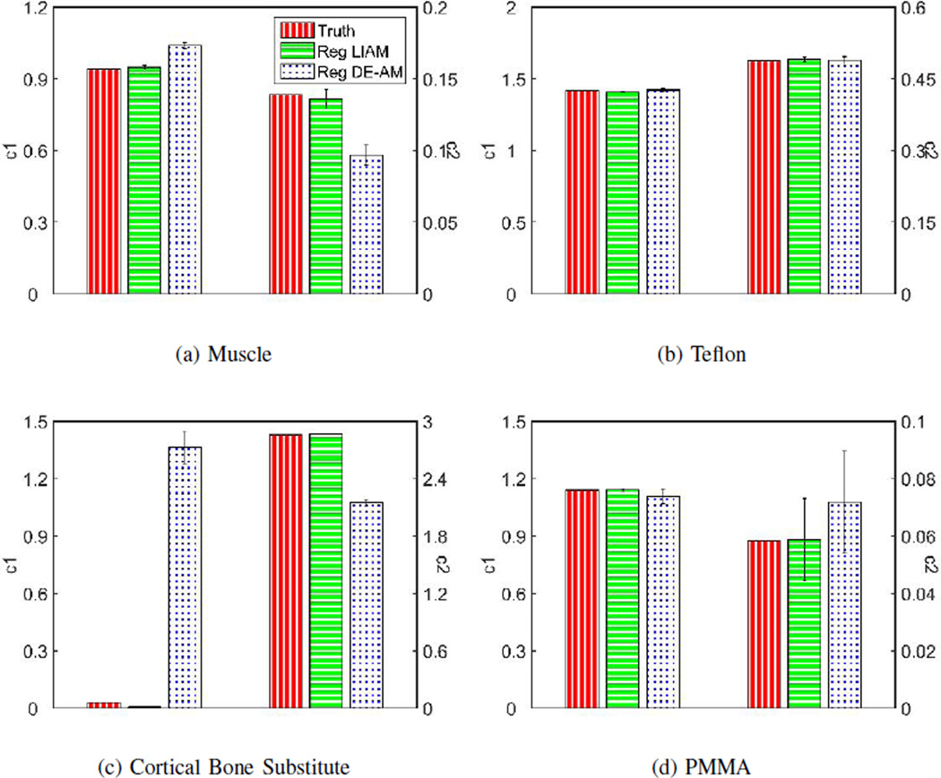
Similar to the unregularized case, we can plot the mean and standard deviation of estimated c1(x) and c2(x) from the regularized LIAM and DE-AM reconstructions with λ = 50 for both reconstructions, as shown in Fig. 6. The reason for selecting reconstructions corresponding to this particular λ value is that among different choices of λ’s, λ = 50 achieves the best image quality (regularized DE-AM is not sensitive to λ ranging from 5 to 500). As is consistent with the unregularized case, regularized LIAM achieves better mean estimation accuracy compared to regularized DE-AM algorithm, and has comparable standard deviations. By jointly looking at Fig. 4, Fig. 5 and Fig. 6, with proper choice of regularization parameters (λ = 50, δ = 500) as well as the incorporation of the projection constraint (β = 1000), regularized LIAM algorithm can achieve much less noise in the reconstructed images while maintaining good accuracy in mean estimation.
Fig. 6.
Mean and standard deviation bar chart of simulated data reconstruction for (a) Muscle, (b) Teflon, (c) Cortical Bone Substitute and (d) PMMA. For regularized LIAM algorithm reconstruction, results were obtained using β → 0 for the first 100 iterations and β = 1000 for the second 100 iterations and λ = 50, δ = 500. For regularized DE-AM algorithm reconstruction, results were obtained using λ = 50, δ = 500 for 25000 iterations without OS.
V. Physical Phantom Experiment Results and Discussions
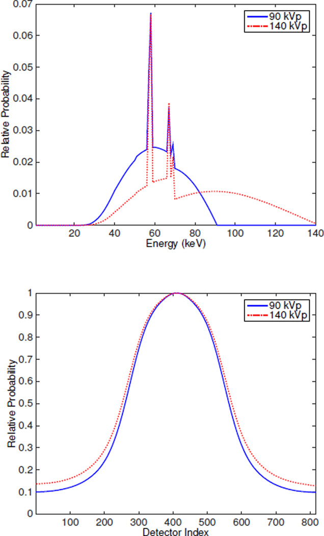
In this section, real data of a cylinder phantom were collected (data were collected by Dong Han and Joshua D. Evans at Virginia Commonwealth University) from the Philips Brilliance Big Bore scanner with 816 detectors per detector row, 1320 sources positions per revolution and collimation 4 by 0.75 mm. Incident spectra are 90 kVp and 140 kVp as shown in Fig. 7 with corresponding bowtie filter which adjusts the rays from each source location to each detector according to its shape. Only the third row of data were used for reconstruction. The physical phantom is a PMMA cylinder with four holes filled with ethanol, teflon, polystyrene and PMMA. The image size is 610 × 610 with pixel size 1 mm × 1 mm. The two component materials used are polystyrene (c1) and calcium chloride solution (c2). The attenuation coefficients spectra for the two components are shown in Fig. 1b.
Fig. 7.
(a) Incident spectra and (b) Bowtie filters for real data from Philips Brilliance Big Bore scanner.
We compute the theoretical truth based on the linear attenuation map from NIST by fitting c1 and c2 according to μ(E) = c1μ1(E) + c2μ2(E). Table II gives the estimated ideal true c1 and c2 for the four sample materials. The nonzero c2 coefficient for polystyrene material is due to the presence of contamination.
TABLE II.
Estimated ideal component coefficients for the physical cylinder phantom.
| Substance | Polystyrene | Calcium Chloride Solution |
|---|---|---|
| PMMA | 1.14 | 0.0583 |
| Ethanol | 0.800 | 0.0337 |
| Teflon | 1.42 | 0.488 |
| Polystyrene | 0.997 | 0.0024 |
A. Reconstruction with β → 0 and Fixed λ
We first test unregularized version of LIAM algorithm with β → 0 on this set of real data. We compare the 100 iteration reconstruction results of unregularized LIAM and the 2500 iteration reconstruction results of unregularized DE-AM with 33 OS (which is equivalent to 82500 iterations without OS). The initial conditions for both of the algorithms are images with all ones.
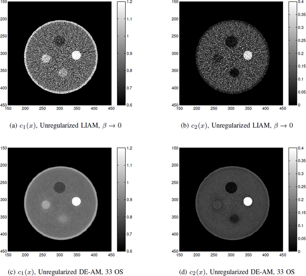
The image reconstruction results are shown in Fig. 8, from which we can see that although the images are all grainy due to the presence of noise, results from unregularized LIAM algorithm can achieve quite accurate estimation of the component images for every region of interest on average. Moreover, LIAM is superior to DE-AM in terms of the number of iterations (100 iterations vs. 2500 iterations with 33 OS). These observations are consistent with those from the simulated noisy data case.
Fig. 8.
Real data reconstructions for (a) c1(x) from unregularized LIAM with β → 0, (b) c2(x) by unregularized LIAM with β → 0, (c) c1(x) from unregularized DE-AM with 33 OS, and (d) c2(x) from unregularized DE-AM with 33 OS.
B. Reconstruction with Dynamic β and λ
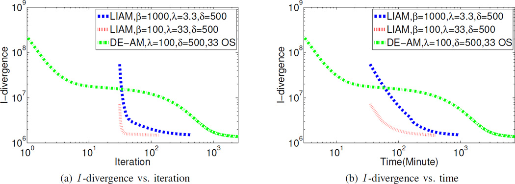
In the following experiments, we compared the reconstruction results from regularized LIAM algorithm and regularized DE-AM algorithm. For regularized DE-AM algorithm, images with all ones were used as the initial condition. Reconstructed images were obtained from 2500 iterations with 33 OS and regularization parameters δ = 500, λ = 100. For regularized LIAM algorithm, images for the initial condition were obtained by using unregularized LIAM algorithm with β → 0 for 30 iterations. The regularized LIAM algorithm with β = 1000 and β = 100 was run for 400 and 100 iterations to obtain the reconstructed images, respectively, based on the convergence plot in Fig. 10. The chosen regularization parameters for regularized LIAM algorithm were δ = 500, λ = 3.3 and λ = 33, respectively.
Fig. 10.
(a) I -divergence vs. iteration and (b) I -divergence vs. time for regularized LIAM algorithm and regularized DE-AM algorithm using real data. I -divergence is evaluated according to (2).
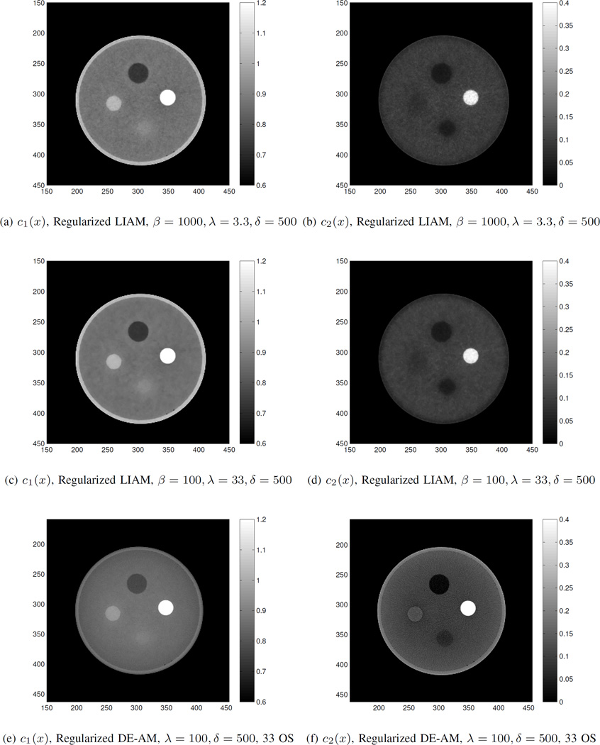
Fig. 9 shows the reconstructed c1(x) and c2(x) images for the three cases described above. By jointly looking at Fig. 8(c)(d) and Fig. 9(e)(f), the results from regularized DE-AM algorithm do not differ significantly from those obtained from unregularized DE-AM algorithm. The introduction of neighborhood penalty in regularized LIAM algorithm has significant smoothness effect in the reconstructed images. For the two reconstructions using regularized LIAM algorithm, the reconstructed images corresponding to β = 100, λ = 33 have less noise in the background.
Fig. 9.
Real data reconstructions for (a) c1(x) from regularized LIAM with β = 1000, λ = 3.3, δ = 500 for 100 iterations, (b) c2(x) from regularized LIAM with β = 1000, λ = 3.3, δ = 500 for 100 iterations, (c) c1(x) from regularized LIAM with β = 100, λ = 33, δ = 500 for 100 iterations, (d) c2(x) from regularized LIAM with β = 100, λ = 33, δ = 500 for 100 iterations, (e) c1(x) from regularized DE-AM with λ = 100, δ = 500, 33 OS for 2500 iterations, and (f) c2(x) from regularized DE-AM with λ = 100, δ = 500, 33 OS for 2500 iterations.
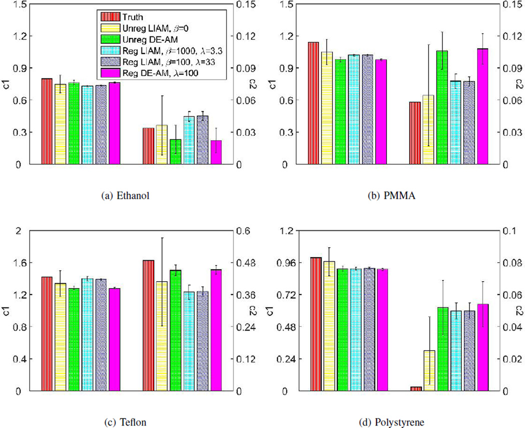
So far, we have used unregularized and regularized LIAM and DE-AM algorithms to reconstruction the same real dataset. Similarly, we can compute the estimated c1(x) and c2(x) means and standard deviation and the corresponding bar charts are shown in Fig. 11. In general, LIAM algorithms can produce better accuracy in mean estimations compared to DE-AM algorithms. We have shown in simulated data case that unregularized LIAM is very sensitive to noise, and regularization is important in order to achieve smooth images. As is consistent with the simulated data case, regularized LIAM, with proper choice of regularization parameters, can produce much less noisy images than unregularized LIAM, without sacrificing much mean estimation accuracy. For the two results using the regularized LIAM algorithm, the case β = 100, λ = 33 has less noise, however, these two choices of β values produce almost identical mean estimations of c1 and c2, which is consistent with observations from Fig. 9.
Fig. 11.
Mean and standard deviation bar chart of real data reconstruction for (a) Ethanol, (b) PMMA, (c) Teflon and (d) Polystyrene. For regularized LIAM algorithm reconstruction, results were obtained using β = 1000, λ = 3.3, δ = 500 and β = 100, λ = 33, δ = 500, respectively, for 100 iterations. For regularized DE-AM algorithm reconstruction, results were obtained using λ = 100, δ = 500 and 33 OS for 2500 iterations.
The c2 overestimation errors for polystyrene insert could have many possible sources, including lack of use scatter correction and off focal radiation and deviations between the actual and assumed photon spectra. We are currently investigating incorporating a more realistic scatter estimate into both the DE-AM and LIAM algorithm in an attempt to mitigate estimation error and image artifacts. Also, as shown by Williamson et al. [8], the single polystyrene-CaCl2 is not an optimally accurate cross section model for low atomic number media. This paper demonstrated that improved accuracy was achievable using a polystyrene-liquid water basis pair for low- Z materials, but at the cost of violating LIAMs nonnegativity constraint. Investigation of these residual estimation errors is currently underway and will be reported in the future.
The evolution of I -divergence (between the data and the mean represented by the reconstructed images) was presented in Fig. 10. Since for regularized LIAM algorithm, the initial condition was obtained after 30 iterations using unregularized LIAM algorithm with β = 0, the corresponding iterations and time are also reflected in the plot. Similar to the simulated data case, the regularized LIAM algorithm converges much faster than regularized DE-AM algorithm, in both iteration and time. According to Fig. 10, it takes regularized LIAM with β = 100, λ = 33 about 200 minutes to converge, while for regularized DE-AM, after 7500 minutes, I -divergence tends to converge to a value that is a little smaller than the value achieved by the regularized LIAM with β = 100, λ = 33 after 200 minutes. With different choices of regularization parameters, convergence time can be different. A smaller β value, for example, β = 100, can achieve faster convergence compared to β = 1000, which takes about 500 min to converge. While not being fully proven, regularized LIAM algorithm not only can achieve monotonic convergence in the total objective function, but also shows monotonic decrease in I -divergence where the mean data are represented by the reconstructed images, not estimated line integrals. Note than in the reconstruction results obtained by using LIAM, in the step of estimating component images from estimated line integrals, an OS method can be used to further reduce computation time.
VI. Conclusions
We have introduced a new algorithm, LIAM, that decouples line integral estimation for two component images from image reconstruction, but utilizes the second step as a soft constraint on the admissible line-integral solutions. This two-step algorithm has much faster convergence than DE-AM algorithm with significantly more accurate and artifact-free component images, even in the presence of high density materials. An edge-preserving penalty function was used as a regularizer in order to achieve desired image smoothness.
To validate the LIAM algorithm, simulated data with and without Poisson noise, as well as real data from the Philips Brilliance Big Bore scanners were used for reconstruction. The DE-AM algorithm was also used for comparison. For the LIAM algorithm, the penalty of the line integral and the forward projections of the component images was first set to zero, and a simple two-step reconstruction by using the ID algorithm was applied after the line integrals were obtained. Compared to DE-AM algorithm, fast convergence was observed and improved average estimation accuracy was achieved. In order to improve image smoothness, a neighborhood penalty was introduced and different regularization parameters were studied to explore the effect on the reconstructed images. Moreover, a nonzero penalty on the line integral and the forward projections of the component images was used in conjunction with a neighborhood penalty to achieve better image smoothness while maintaining quantitatively accurate estimates. By using only a small fraction of the computation time of DE-AM, LIAM achieves better accuracy of the component coefficients estimations in the presence of Poisson noise for simulated data reconstruction and achieves the same level of accuracy in the component coefficients estimations for real data reconstruction. In the future experiments, an OS method can be applied in the step where one tries to estimate the component images from the estimated line integrals, such that even faster convergence can be obtained.
In summary, the LIAM algorithm can achieve fast convergence without sacrificing the estimation accuracy, making its clinical application possible. With proper choices of regularization parameters, which can be obtained empirically, good reconstructed image quality and accurate estimates of component coefficients can be achieved.
There are detectors available that provide energy-sensitive, often photon-counting measurements. These may open a pathway toward the development of medical imaging systems that provide improved volumetric, quantitative data about material properties. The LIAM algorithm can be applied directly to such spectral CT systems, with varying numbers of measurement energy bins and material bases.
Acknowledgments
The authors thank the reviewers for their comments that helped significantly improve the presentation in the paper. We thank Mariela A. Porras-Chaverri for her input to the introduction. This work was supported in part from Grant No. R01CA 75371awarded by the National Institutes of Health.
Appendix
Since the objective function is decoupled in every , for simplification, we use ĉold to denote and ĉnew to denote . The following pseudocode is to replace step D in the unregularized LIAM pseudocode and is denoted by D’.
D’. Calculate ĉnew using the trust region Newton’s method.
|
Step b in D’ is to enforce nonnegativity for the component images. The choices of η1, η2, γ1, γ2 and Δ(n=0) are empirical. We used η1 = 0.1, η2 = 0.9, γ1 = 0.5, γ2 = 2, Δ(n=0) = 0.25 for our implementation of trust region Newton’s method.
Contributor Information
Yaqi Chen, Department of Electrical and Systems Engineering, Washington University in St. Louis, St. Louis, MO, 63130 USA.
Joseph A. O’Sullivan, Department of Electrical and Systems Engineering, Washington University in St. Louis, St. Louis, MO, 63130 USA.
David G. Politte, Electronic Radiology Laboratory, Mallinckrodt Institute of Radiology, Washington University School of Medicine, St. Louis MO, 63110.
Joshua D. Evans, Department of Radiation Oncology, Virginia Commonwealth University, Richmond, VA, 23220
Dong Han, Department of Radiation Oncology, Virginia Commonwealth University, Richmond, VA, 23220.
Bruce R. Whiting, Department of Radiology, University of Pittsburgh, Pittsburgh, PA, 15213
Jeffrey F. Williamson, Department of Radiation Oncology, Virginia Commonwealth University, Richmond, VA, 23220
References
- 1.du Plessis FCP, Wilemse CA, Lotter MG. The indirect use of CT numbers to establish material properties needed for Monte Carlo calculation of dose distributions in patients. Medical Physics. 1998;25(7):1195–1201. doi: 10.1118/1.598297. [DOI] [PubMed] [Google Scholar]
- 2.Schneider U, Pedroni E, Lomax A. The calibration of CT Hounsfield units for radiotherapy treatment planning. Physics in Medicine and Biology. 1996;41(1):111–124. doi: 10.1088/0031-9155/41/1/009. [DOI] [PubMed] [Google Scholar]
- 3.Yang M, Virshup G, Clayton J, Zhu XR, Mohan R, Dong L. Theoretical variance analysis of single- and dual-energy computed tomography methods for calculating proton stopping power ratios of biological tissues. Physics in Medicine and Biology. 2010;55(5):1343–1362. doi: 10.1088/0031-9155/55/5/006. [DOI] [PubMed] [Google Scholar]
- 4.I. C. on Radiological Protection. Report on the Task Group on Reference Man. Oxford: Pergamon Press; 1975. [Google Scholar]
- 5.Beaulieu L, Tedgren AC, Carrier JF, Davis SD, Mourtada F, Rivard MJ, Thomson RM, Verhaegen F, Wareing TA, Williamson JF. Report of the Task Group 186 on model-based dose calculation methods in brachytherapy beyond the TG-43 formalism: current status and recommendations for clinical implementation. Medical Physics. 2012;39(10):6208–6236. doi: 10.1118/1.4747264. [DOI] [PubMed] [Google Scholar]
- 6.Sechopoulos I, Suryanarayanan S, Vedantham S, D’Orsi C, Karellas A. Computation of the glandular radiation dose in digital tomosynthesis of the breast. Medical Physics. 2007;34(1):221–232. doi: 10.1118/1.2400836. [DOI] [PMC free article] [PubMed] [Google Scholar]
- 7.Rutherford RA, Pullan BR, Isherwood I. Measurement of effective atomic number and electron density using an EMI scanner. Neuroradiology. 1976;11(1):15–21. doi: 10.1007/BF00327253. [DOI] [PubMed] [Google Scholar]
- 8.Williamson JF, Li S, Devic S, Whiting BR, Lerma FA. On two parameter models of photon cross sections: application to dualenergy CT imaging. Medical Physics. 2006 Nov;33(11):4115–4129. doi: 10.1118/1.2349688. [DOI] [PubMed] [Google Scholar]
- 9.Torikoshi M, Tsunoo T, Sasaki M, Endo M, Noda Y, Ohno Y, Kohno T, Hyodo K, Uesugi K, Yagi N. Electron density measurement with dual-energy X-ray CT using synchrotron radiation. Physics of Medicine and Biology. 2003;48(5) doi: 10.1088/0031-9155/48/5/308. [DOI] [PubMed] [Google Scholar]
- 10.Evans JD, Whiting BR, O’Sullivan JA, Politte DG, Klahr PF, Yu Y, Williamson JF. Prospects for in vivo estimation of photon linear attenuation coefficients using postprocessing dual-energy CT imaging on a commercial scanner: comparison of analytic and polyenergetic statistical reconstruction algorithms. Medical Physics. 2013;40(12):121914. doi: 10.1118/1.4828787. [DOI] [PMC free article] [PubMed] [Google Scholar]
- 11.Zhang R, Thibault J-B, Bouman CA, Sauer KD, Hsieh J. An iterative maximum-likelihood polychromatic algorithm for CT. IEEE Transactions on Medical Imaging. 2001 Oct;20(10):999–1008. doi: 10.1109/42.959297. [DOI] [PubMed] [Google Scholar]
- 12.Beister M, Kolditz D, Kalender WA. Iterative reconstruction methods in X-ray CT. Physica Medica. 2012 Feb;28(2):94–108. doi: 10.1016/j.ejmp.2012.01.003. [DOI] [PubMed] [Google Scholar]
- 13.Fessler JA. Statistical image reconstruction methods for transmission tomography. In: Sonka M, Fitzpatrick JM, editors. Medical Image Processing and Analysis. Vol. 2. SPIE Press; 2000. [Google Scholar]
- 14.Elbakri IA, Fessler JA. Efficient and accurate likelihood for iterative image reconstruction in X-ray computed tomography. Proc. of SPIE 5032. Medical Imaging 2003: Image Processing. 2003:1839–1850. [Google Scholar]
- 15.Erdogan H, Fessler JA. Monotonic algorithms for transmission tomography. IEEE Transactions on Medical Imaging. 1999 Sep;18(9):801–814. doi: 10.1109/42.802758. [DOI] [PubMed] [Google Scholar]
- 16.Thibault J-B, Sauer KD, Bouman CA, Hsieh J. A three-dimensional statistical approach to improved image quality for multislice helical CT. Medical Physics. 2007 Nov;34(11):4526–4544. doi: 10.1118/1.2789499. [DOI] [PubMed] [Google Scholar]
- 17.Snyder DL, O’Sullivan JA, Murphy RJ, Politte DG, Whiting BR, Williamson JF. Image reconstruction for transmission tomography when projection data are incomplete. Physics in Medicine and Biology. 2006;51(21):5603–5619. doi: 10.1088/0031-9155/51/21/015. [DOI] [PubMed] [Google Scholar]
- 18.Williamson JF, Whiting BR, Benac J, Murphy RJ, Blaine GJ, O’Sullivan JA, Politte DG, Synder DL. Prospects for quantitative computed tomography imaging in the presence of foreign metal bodies using statistical image reconstruction. Medical Physics. 2002;29(10):2402–2408. doi: 10.1118/1.1509443. [DOI] [PubMed] [Google Scholar]
- 19.Evans JD, Politte DG, Whiting BR, O’Sullivan JA, Williamson JF. Noise-resolution tradeoffs in X-ray CT imaging: a comparison of penalized alternating minimization and filtered backprojection algorithms. Medical Physics. 2011;38(3):1444–1458. doi: 10.1118/1.3549757. [DOI] [PMC free article] [PubMed] [Google Scholar]
- 20.O’Sullivan JA, Benac J. Alternating minimization algorithms for transmission tomography. IEEE Transactions on Medical Imaging. 2007 Mar;26(3):283–297. doi: 10.1109/TMI.2006.886806. [DOI] [PubMed] [Google Scholar]
- 21.Evans JD, Whiting BR, Politte DG, O’Sullivan JA, Klahr PF, Williamson JF. Experimental implementation of a polyenergetic statistical reconstruction algorithm for a commercial fan-beam CT scanner. Physica Medica. 2013;29(5):500–512. doi: 10.1016/j.ejmp.2012.12.005. [DOI] [PMC free article] [PubMed] [Google Scholar]
- 22.Alvarez RE, Macovski A. Energy-selective reconstructions in X-ray computerized tomography. Medical Physics. 1976;21:733–744. doi: 10.1088/0031-9155/21/5/002. [DOI] [PubMed] [Google Scholar]
- 23.Heismann BJ. Signal-to-noise Monte-Carlo analysis of base material decomposed CT projections. Nuclear Science Symposium Conference Record; IEEE; 2006. pp. 3174–3175. [Google Scholar]
- 24.Kalender WA, Klotz E, Kostaridou L. An algorithm for noise suppression in dual energy CT material density images. IEEE Transactions on Medical Imaging. 2008;7(3):218–224. doi: 10.1109/42.7785. [DOI] [PubMed] [Google Scholar]
- 25.Fessler JA, and IE. Maximum-likelihood dual-energy tomographic image reconstruction. Proceedings of SPIE. 2002 Feburary;:38–49. [Google Scholar]
- 26.Zhang R, Thibault J-B, Bouman CA, Sauer KD, Hsieh J. Model-based iterative reconstruction for dual-energy X-ray CT using a joint quadratic likelihood model. IEEE Transactions on Medical Imaging. 2014 Jan;33(1):117–134. doi: 10.1109/TMI.2013.2282370. [DOI] [PubMed] [Google Scholar]
- 27.Heismann B, Schmidt B, Flohr T. Spectral computed tomography. Bellingham, Washington, USA: SPIE Press; 2012. [Google Scholar]
- 28.Noh J, Fessler JA, Kinahan PE. Statistical sinogram restoration in dual-energy CT for PET attenuation correction. IEEE Transactions on Medical Imaging. 2009;28(11):1688–1702. doi: 10.1109/TMI.2009.2018283. [DOI] [PMC free article] [PubMed] [Google Scholar]
- 29.Benac J. Ph.D. dissertation. St. Louis, Missouri: Washington University in St. Louis; 2005. Alternating minimization algorithms for X-ray computed tomography: Multigrid acceleration and dual energy. [Google Scholar]
- 30.Chen Y, Moran CH, Tan Z, Wooten AL, O’Sullivan JA. Robust analysis of multiplexed SERS microscopy of Ag nanocubes using an alternating minimization algorithm. Raman Spectroscopy. 2013 Feb;44:703–709. [Google Scholar]
- 31.O’Sullivan JA, Benac J, Williamson JF. Alternating minimization algorithms for dual energy X-ray CT; Biomedical Imaging: Nano to Macro, 2004. IEEE International Symposium; 2004. pp. 579–582. [Google Scholar]
- 32.Jang KE, Lee J, Sung Y, Lee S. Information-theoretic discrepancy based iterative reconstructions (IDIR) for polychromatic X-ray tomography. Medical Physics. 2013 Aug;40(11):091908. doi: 10.1118/1.4816945. [DOI] [PubMed] [Google Scholar]
- 33.Chen Y. Ph.D. dissertation. St. Louis, Missouri: Washington University in St. Louis; 2014. Alternating minimization algorithms for dual-energy Xray CT imaging and information optimization. http://openscholarship.wustl.edu/etd/1291. [Google Scholar]
- 34.Afonso MV. Fast image recovery using variable splitting and constrained optimization. IEEE Transactions on Image Processing. 2010 Apr;19(9):2345–2356. doi: 10.1109/TIP.2010.2047910. [DOI] [PubMed] [Google Scholar]
- 35.Goldstein T, Osher S. The split Bregman method for L1- regularized problems. SIAM Journal on Imaging Sciences. 2009;2(2):323–343. [Google Scholar]
- 36.Rockafellar RT. The multiplier method of Hestenes and Powell applied to convex programming. Journal of Optimization Theory and applications. 1973;12(6):555–562. [Google Scholar]
- 37.Boyd S, Parikh N, Chu E, Peleato B, Eckstein J. Distributed optimization and statistical learning via the alternating direction method of multipliers. Foundations and Trends in Machine Learning. 2011;3(1):1–122. [Google Scholar]
- 38.Csiszár I. I-divergence geometry of probability distributions and minimization problems. The Annals of Probability. 1975:146–158. [Google Scholar]
- 39.Csiszár I. Why least squares and maximum entropy? an axiomatic approach to inference for linear inverse problems. The annals of statistics. 1991:2032–2066. [Google Scholar]
- 40.Nien H, Fessler J, et al. Fast X-ray CT image reconstruction using a linearized augmented lagrangian method with ordered subsets. Medical Imaging, IEEE Transactions on. 2015;34(2):388–399. doi: 10.1109/TMI.2014.2358499. [DOI] [PMC free article] [PubMed] [Google Scholar]
- 41.Ramani S, Fessler J, et al. A splitting-based iterative algorithm for accelerated statistical X-ray CT reconstruction. Medical Imaging, IEEE Transactions on. 2012;31(3):677–688. doi: 10.1109/TMI.2011.2175233. [DOI] [PMC free article] [PubMed] [Google Scholar]
- 42.Tracey BH, Miller EL. Stabilizing dual-energy X-ray computed tomography reconstructions using patch-based regularization. arXiv:cs. 2014 vol. arXiv: 1403.6318. [Google Scholar]
- 43.Sawatzky A, Xu Q, Schirra CO, Anastasio M, et al. Proximal admm for multi-channel image reconstruction in spectral X-ray CT. Medical Imaging, IEEE Transactions on. 2014;33(8):1657–1668. doi: 10.1109/TMI.2014.2321098. [DOI] [PubMed] [Google Scholar]
- 44.Wang H, Banerjee A. Bregman alternating direction method of multipliers. arXiv:math. 2014 vol. arXiv: 1306.3203v3. [Google Scholar]
- 45.Snyder DL, Schulz TJ, O’Sullivan JA. Deblurring subject to nonnegativity constraints. IEEE Transactions on Signal Processing. 1992 May;40(5):1143–1150. [Google Scholar]
- 46.Whiting BR. Signal statistics in X-ray computed tomography. Medical Imaging 2002. International Society for Optics and Photonics. 2002:53–60. [Google Scholar]
- 47.Whiting BR, Massoumzadeh P, Earl OA, O’Sullivan JA, Snyder DL, Williamson JF. Properties of preprocessed sinogram data in X-ray computed tomography. Medical physics. 2006;33(9):3290–3303. doi: 10.1118/1.2230762. [DOI] [PubMed] [Google Scholar]
- 48.Lasio GM, Whiting BR, Williamson JF. Statistical reconstruction for X-ray computed tomography using energy-integrating detectors. Phys. Med. Biol. 2007;52:2247–2266. doi: 10.1088/0031-9155/52/8/014. [DOI] [PubMed] [Google Scholar]
- 49.Lange K. Convergences of EM image reconstruction algorithms with Gibbs smoothing. IEEE Transactions on Medical Imaging. 1990;4:439–446. doi: 10.1109/42.61759. [DOI] [PubMed] [Google Scholar]
- 50.Erdogan H, Fessler JA. Ordered subsets algorithms for transmission tomography. Physics in Medicine and Biology. 1999 Jul;44:2835–2851. doi: 10.1088/0031-9155/44/11/311. [DOI] [PubMed] [Google Scholar]
- 51.Fessler JA, Ficaro EP, Clinthome NH, Lange K. Grouped-coordinate ascent algorithms for penalized-likelihood transmission image reconstruction. IEEE Transactions on Medical Imaging. 1997:166–175. doi: 10.1109/42.563662. [DOI] [PubMed] [Google Scholar]
- 52.De Pierro AR. A modified expectation maximization algorithm for penalized likelihood estimation in emission tomography. IEEE transactions on medical imaging. 1994;14(1):132–137. doi: 10.1109/42.370409. [DOI] [PubMed] [Google Scholar]
- 53.Sorensen DC. Newton’s method with a model trust region modification. SIAM Journal on Numerical Analysis. 1982;19(2):409–426. [Google Scholar]
- 54.Nowotny R, Hofer A. Program for calculating diagnostic Xray spectra. RoeFo, Fortschr. Geb. Roentgenstr. Nuklearmed. 1985;142(6):685–689. doi: 10.1055/s-2008-1052738. [DOI] [PubMed] [Google Scholar]


