Abstract
Diffusion MRI affords valuable insights into white matter microstructures, but suffers from low signal-to-noise ratio (SNR), especially at high diffusion weighting (i.e., b-value). To avoid time-intensive repeated acquisition, post-processing algorithms are often used to reduce noise. Among existing methods, non-local means (NLM) has been shown to be particularly effective. However, most NLM algorithms for diffusion MRI focus on patch matching in the spatial domain (i.e., x-space) and disregard the fact that the data live in a combined 6D space covering both spatial domain and diffusion wavevector domain (i.e., q-space). This drawback leads to inaccurate patch matching in curved white matter structures and hence the in-ability to effectively use recurrent information for noise reduction. The goal of this paper is to overcome this limitation by extending NLM to the joint x – q space. Specifically, we define for each point in the x – q space a spherical patch from which we extract rotation-invariant features for patch matching. The ability to perform patch matching across q-samples allows patches from differentially orientated structures to be used for effective noise removal. Extensive experiments on synthetic, repeated-acquisition, and HCP data demonstrate that our method outperforms state-of-the-art methods, both qualitatively and quantitatively.
Keywords: Denoising, Diffusion MRI, Non-local means, Patch matching
1. Introduction
Diffusion MRI (DMRI) relies on its sensitivity to the displacement of water molecules to probe tissue microstructure. To be able to characterize fine microstructural details, the diffusion weighting (i.e., b-value) needs to be sufficiently high, allowing, for example, more accurate separation of fiber bundles crossing at small angles and greater sensitivity to the restricted diffusion of water molecules trapped inside axons. However, due to the significant attenuation of the MR signal at high diffusion weightings, the low signal-to-noise ratio (SNR) poses significant challenges to subsequent analysis.
A straightforward means to improve SNR is by repeating and averaging scans (Johansen-Berg and Behrens, 2013), which however inevitably prolongs acquisition times and is hence impractical in clinical settings. In view of this, post-acquisition denoising methods have been widely adopted (Wiest-Daesslé et al., 2007, 2008; Descoteaux et al., 2008; Becker et al., 2012; Manjón et al., 2013; Becker et al., 2014; Lam et al., 2014; Yap et al., 2014; Varadarajan and Haldar, 2015; Veraart et al., 2016; St-Jean et al., 2016; Chen et al., 2019). Among existing methods, non-local means (NLM) (Buades et al., 2005) has been shown to be particularly good at preserving edges when reducing noise. NLM avoids blurring by averaging over recurrent image patterns collected via patch matching.
NLM has been applied to reducing noise in DMRI data (Wiest-Daesslé et al., 2007, 2008; Descoteaux et al., 2008; Yap et al., 2014). Existing NLM methods denoise diffusion-weighted (DW) images as individual images, a multi-spectral vector image, or parametric maps given by a diffusion model (Wiest-Daesslé et al., 2007). However, these methods mainly focus on patch matching in the spatial domain (i.e., x-space), despite the fact that DMRI data live in a combined space consisting of both spatial x-space and diffusion wavevector q-space. This causes NLM to be less effective in locating self-similar patterns in highly curved white matter structures, resulting in smoothing artifacts caused by averaging over differentially oriented structures. Another limitation of NLM is the rare patch effect (Duval et al., 2011; Deledalle et al., 2012; Salmon and Strozecki, 2012). This phenomenon happens when matching structures cannot be found, leading to the degradation of fine details and causing halos around object boundaries. A natural solution to this problem is to expand the search extent (Prima and Commowick, 2013; Chen et al., 2016c) so that the possibility of finding matching structures can be increased. However, this significantly increases computation time and might result in false-positive matches.
To overcome these limitations, in this paper we extend NLM beyond x-space to include q-space for improved denoising in DMRI. Specifically, for each point in x – q space, we first define a patch covering a q-space neighborhood. We then perform patch matching in x – q space and assign a weight, indicating neighborhood similarity, for each pair of points in the joint space. Finally, the denoised signal at each point in x – q space is estimated via weighted averaging.
The advantage afforded by this extension is fourfold: (i) Non-local information can now be harnessed not only over x-space, but also over q-space, allowing information to be borrowed across DW images for effective denoising; (ii) Information from structures oriented in different directions can be used more effectively for denoising without introducing artifacts; (iii) Patch matching complexity can be significantly reduced by leveraging the fact that diffusion signal profiles generally have smooth and simpler shapes; (iv) The simpler shapes also imply that better patch matches can be found more easily, therefore mitigating the rare patch effect.
Before noise reduction, we first transform the DMRI data, using Koay’s inversion technique (St-Jean et al., 2016; Koay et al., 2009a), so that noise is Gaussian-distributed. This is essential for DMRI data acquired using modern multi-coil MRI techniques, which typically exhibit stationary/non-stationary Rician/noncentral χ (nc-χ) noise distributions.
Comprehensive experiments on synthetic, repeated-acquisition, and HCP data demonstrate that x – q space non-local means (XQ-NLM) removes noise effectively while preserving structures and improves the quality of derived quantities, such as generalized fractional anisotropy (GFA) (Tuch, 2004), orientation distribution function (ODF), and fiber tracts. We compared our method with state-of-the-art methods, including adaptive NLM (ANLM) (Manjón et al., 2010), non-local spatial and angular matching (NL-SAM) (St-Jean et al., 2016), and Marchenko-Pastur principle component analysis (MPPCA) (Veraart et al., 2016). Experimental results confirm that our method consistently gives the best performance both qualitatively and quantitatively.
A preliminary version of this work has been presented at a conference (Chen et al., 2016a). In this journal version, we (i) extend our method to work with a wider range of noise types resulting from multi-coil MRI and different methods of magnitude signal reconstruction, (ii) perform quantitative evaluation using a ground truth generated using repeatedly acquired data, (iii) include new results for synthetic and real data with additional metrics covering voxel- and tract-based assessments, (iv) compare our method with state-of-the-art denoising methods (i.e., NLSAM and MPPCA), and (v) include additional discussions that are not part of the conference publication.
The rest of the paper is organized as follows. We will first flesh out in Section 2 the key components of the proposed method. We will then demonstrate the effectiveness of our method in Section 3 using synthetic and real data. Additional discussions are provided in Section 4 before concluding the paper in Section 5.
2. Methods
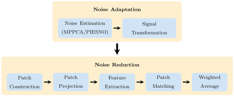
Our method consists of two major components, i.e., noise adaptation and noise reduction. We first transform the signal for Gaussian-distributed noise and then remove noise using x – q space non-local means. An overview of our method is shown in Fig. 1.
Fig. 1.
Method overview.
2.1. Noise adaptation
2.1.1. Noise types in multi-coil MRI
The noise distribution of the composite magnitude signal (CMS) (Aja-Fernández and Vegas-Sánchez-Ferrero, 2016) given by modern multi-coil MRI techniques is dependent on how the k-space signal is sampled and how it is used to reconstruct the magnitude signal. For practical purposes, it is commonly assumed that noise in the real and imaginary parts of k-space is generated using a zero-mean stationary Gaussian process with equal variance (Gudbjartsson and Patz, 1995; Aja-Fernández and Vegas-Sánchez-Ferrero, 2016).
Sum of squares (SoS) and spatial matched filter (SMF) are widely used for CMS reconstruction. For N coils with uncorrelated noise, SoS reconstruction from fully-sampled k-space data leads to spatially stationary nc-χ noise distribution with 2N degrees of freedom, whereas SMF leads to spatially stationary Rician noise distribution (Dietrich et al., 2008). If noise is correlated across coils, the noise distribution of the reconstructed CMS becomes spatially non-stationary.
To accelerate acquisition, parallel MRI subsamples the k-space. Two widely used methods are sensitivity encoding (SENSE) (Pruessmann et al., 1999) and generalized autocalibrating partially parallel acquisition (GRAPPA) (Griswold et al., 2002). The CMS reconstructed by SENSE follows a non-stationary Rician distribution (Aja-Fernández et al., 2014). The noise of the CMS reconstructed from GRAPPA data using SoS and SMF follows the non-stationary nc-χ and Rician distributions, respectively (Aja-Fernández et al., 2014).
2.1.2. Signal transformation
Before denoising, we transform the CMS so that its noise becomes Gaussian-distributed, similar to St-Jean et al. (2016). This involves estimating the location parameter and Gaussian noise standard deviation of the nc-χ distribution and then performing signal transformation using the nc-χ cumulative distribution function (CDF) and the inverse Gaussian CDF (Koay et al., 2009a). Such signal transformation reduces the complexity of the denoising algorithm by not having to deal with the nc-χ nature of the noise (St-Jean et al., 2016; Koay et al., 2009a).
The estimation of noise standard deviation is key to accurate signal transformation. For spatially stationary noise, the noise standard derivation can be estimated from the image background via a method called probabilistic identification and estimation of noise (PIESNO) (Koay et al., 2009b). For spatially non-stationary noise, a number of methods can be used (Manjón et al., 2010; St-Jean et al., 2016; Manjón et al., 2013; Veraart et al., 2016). For instance, adaptive NLM (ANLM) (Manjón et al., 2010) and NLSAM (St-Jean et al., 2016) estimate the noise standard deviation using self-recurrent information. The local PCA method (Manjón et al., 2013) introduces noise estimators for single (SIBE) or multiple (MUBE) baseline (b = 0 s/mm2) images. MUBE performs PCA decomposition on multiple baseline images and then uses the noise PCA component to estimate the noise standard deviation. SIBE uses a similar strategy, but performs PCA decomposition on DW images. Using random matrix theory, the Marchenko-Pastur distribution can be used to determine an appropriate eigenvalue threshold for determining the noise PCA components (Veraart et al., 2016). This method, called MPPCA (Veraart et al., 2016), simultaneously estimates the threshold and the noise standard deviation. The nc-χ bias in the estimated noise standard deviation is corrected using the method described in Koay and Basser (2006). In this work, we use PIESNO and MPPCA, respectively, for stationary and non-stationary noise estimation.
2.2. Noise reduction
2.2.1. x – q space non-local means
We propose to utilize patch matching in both x-space and q-space for effective denoising. For each voxel at location , the diffusion-attenuated signal measurement S(xi, qk) corresponding to wavevector is denoised by averaging over non-local measurements with similar neighborhoods. Note that the signal is Gaussian-distributed after the transformation described in the previous section. We estimate the denoised signal as
| (1) |
where is the search neighborhood in x – q space associated with (xi, qk), w[i, k; j, l] is the weight indicating the q-patch similarity between (xi, qk) and (xj, ql), which is determined using patch matching as described next.
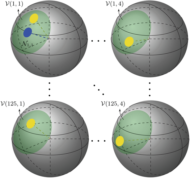
Instead of restricting patch matching to x-space (Wiest-Daesslé et al., 2007, 2008; Descoteaux et al., 2008; Yap et al., 2014), we introduce x – q space patch matching via patches defined in q-space. For each point in x – q space (xi, qk) we define a spherical patch, , centered at qk with fixed qk = ∣qk∣ and subject to a neighborhood angle αp. The samples on this spherical patch are mapped onto a disc using azimuthal equidistant projection (AEP, Section 2.2.2) before computing rotation invariant features via polar complex exponential transform (PCET, Section 2.2.3) for patch matching. Fig. 2 illustrates how patch matching is carried out in x – q space. The search radius in x-space is s (2s + 1 in diameter) and the search angle in q-space is αs. Matching between different shells is allowed.
Fig. 2.
Patch Matching in x – q Space. Illustration of patch matching involving 4 shells in q-space and a search radius of 2 voxels (5 voxels in diameter) in x-space. The search neighborhood is a combination of the sub-neighborhoods (green) associated with different locations {xj}j=1, …,53 and b-values {br}r=1, …,,4, i.e., , where . Patch matching is carried out between the reference patch (blue) and each candidate patch (yellow) in the search neighborhood . (For interpretation of the references to color in this figure legend, the reader is referred to the web version of this article.)
In practice, q-space is not always sampled in a shell-like manner. In this case, we project measurement samples onto spherical patches. Each sampling point in q-space (xi, qk) can be seen as defining a virtual shell with radius ∣qk∣. We project the signals onto this shell to form for patch matching. This is done for example by projecting the signal measured at (xi, qk′), i.e., S(xi, qk′), to , taking a value that is modulated by an exponential function of difference in b-values, i.e.,
| (2) |
where bk = t∣qk∣2 and bk′ = t∣qk′∣2 are the respective b-values, t is the diffusion time. The contribution of S(xi, qk′) is controlled by hprojection.
2.2.2. Azimuthal equidistant projection (AEP)
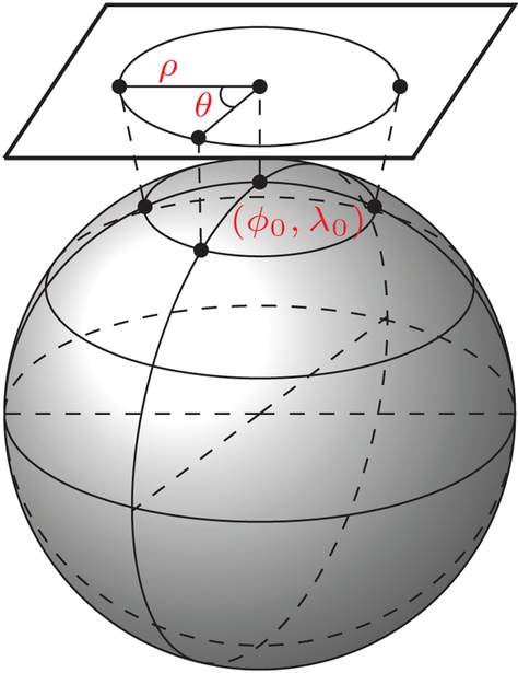
Before feature computation, we first project each spherical patch onto a disc using AEP (Wessel and Smith, 2001). This provides a good basis for subsequent computation of invariant features for matching. The AEP is selected due to its ability to map the coordinates on a sphere to a plane where the distances and azimuths of points on the sphere are preserved with respect to a reference point (Wessel and Smith, 2001). The reference point, which in our case corresponds to the center of a spherical patch, will project to the center of a disc. As illustrated in Fig. 3, viewing the reference point as the ‘North pole’, all points along a given azimuth θ will project along a straight line from the center of the disc. In the projection plane, this line subtends an angle θ with a “vertical” line delineating θ = 0. The distance from the center to another projected point is given as ρ. We represent the reference point as spherical coordinates (ϕ0, λ0), with ϕ referring to latitude and λ referring to longitude. We project (ϕ, λ) to a corresponding point (ρ, θ) in a 2D polar coordinate system, where ρ is the radius and θ is the angle. Based on Wessel and Smith (2001), the relationship between (ϕ, λ) and (ρ, θ) is as follows:
| (3a) |
| (3b) |
Fig. 3.
Azimuthal Equidistant Projection (AEP). Mapping of a spherical patch to a disc.
The projection can be described as a two-step mapping:
| (4) |
AEP maps a q-space spherical patch to a 2D circular patch . Note that AEP changes only the coordinates but not the actual values of the signal vector. If we let be a vector containing the values of all diffusion signals in , then .
Note that extra care needs to be taken when using the above equations to take into consideration the fact that diffusion signals are antipodal symmetric. Prior to performing AEP, we map antipodally all the points on the sphere to the hemisphere where the reference point is located.
2.2.3. Polar complex exponential transform (PCET)
After AEP, we proceed with the computation of rotation invariant features. We choose to use the polar complex exponential transform (PCET) (Yap et al., 2010) for its computation efficiency and its rotation-invariance property as demonstrated in Yap et al. (2010). Rotation invariance allows matching of patches that have different orientations. Denoting an element of as S(x, q, ρ, θ), the PCET of order n, ∣n∣ = 0, 1, 2, …, ∞, and repetition l, ∣l∣ = 0, 1, 2, …, ∞, is defined as
| (5) |
where [·]* denotes the complex conjugate and Hn,l(ρ, θ) is the basis function defined as Hn,l(ρ, θ) = ei2πnρ2 eilθ. It can be easily verified that is invariant to rotation (Yap et al., 2010). Interested readers are referred to Yap et al. (2010) for mathematical and implementation details. up to maximum order m, i.e., −m ≤ l, n ≤ m, are concatenated into a feature vector .
2.2.4. Patch matching
Let be the feature vector of the projected patch , the matching weight w[i, k; j, l] is defined as
| (6) |
with
| (7) |
| (8) |
where Zi,k is a normalization constant to ensure that the weights sum to one:
| (9) |
Here hM(i, k) is a parameter controlling the attenuation of the first exponential function. As in Coupé et al. (2008), we set , where βM is a constant (Coupé et al., 2008) and is the noise standard deviation. Similarly, controls the attenuation of the other exponential function, where σb is a scale parameter.
3. Experiments
3.1. Datasets
3.1.1. Synthetic data
For quantitative evaluation, a synthetic multi-shell dataset was generated using Phantomαs (Caruyer et al., 2014), a toolbox for simulating DMRI data with complex fiber geometries. We use the geometric model designed for ISBI 2013 HARDI challenge,1 which consists of various configurations such as branching, crossing, and kissing. The parameters used for data simulation were chosen to be consistent with the real data described in Section 3.1.3: b = 1000, 2000, 3000 s/mm2, 90 gradient directions per shell, 55 × 55 voxels with resolution 2 × 2 mm2.
Stationary and non-stationary nc-χ noise with 1, 4, and 8 channels and level 5%, 7.5%, 10% was added to the data. For an N-channel receiver coil, the measured signal YN with nc-χ noise is given by (Constantinides et al., 1997; Koay and Basser, 2006; Koay et al., 2009a)
| (10) |
where μR(k) and μI(k) are respectively the real and imaginary parts of the true complex signal from the kth channel. XR(k) and XI(k) are two random variables that follow the same Gaussian distribution with standard deviation and . In the absence of noise, the true signal μN can be expressed as
| (11) |
The nc-χ distribution depends only on μN and not the actual signals from the individual channels. Therefore, the noisy signal can be generated by
| (12) |
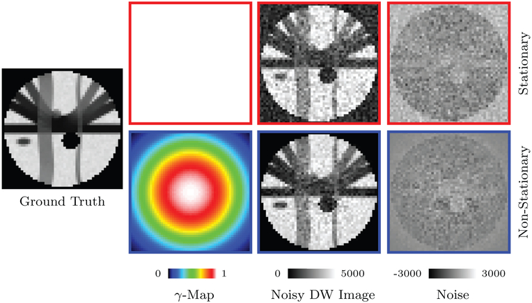
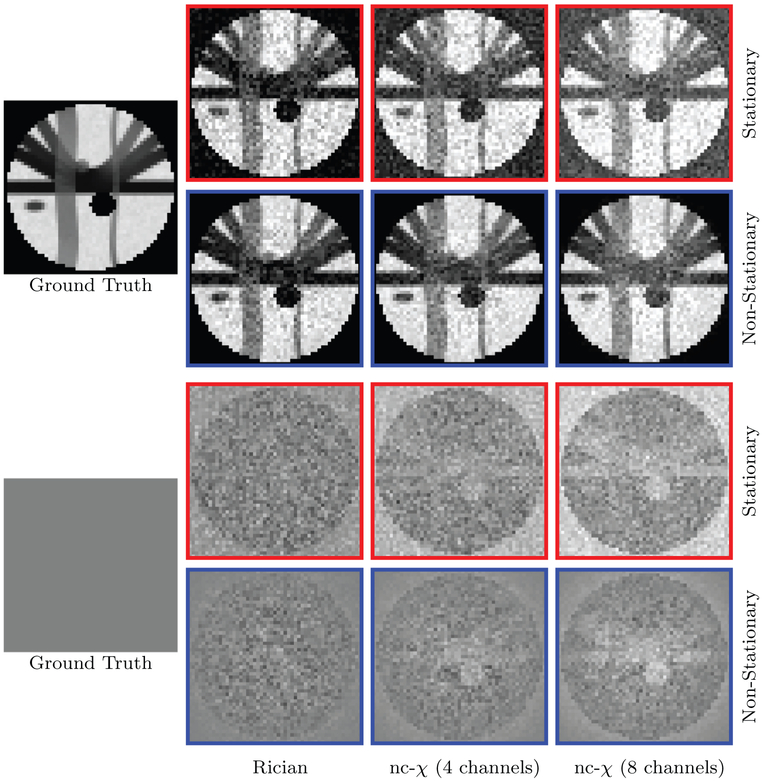
The number of channels affects the noise distribution and the severity of noise floor (Aja-Fernández and Vegas-Sánchez-Ferrero, 2016). For stationary noise, we set γ = 1. For nonstationary noise, γ varies spatially. We set σ as p percent of the maximum data intensity value v, i.e., σ = v(p/100). Examples of stationary and non-stationary γ-maps used in this work are shown in Fig. 4. Example images for different numbers of channels are shown in Fig. 5.
Fig. 4.
Noise Simulation. 5% 4-channel nc-χ noise with spatially constant and varying γ-maps. Note that the γ-map for stationary noise is constant. DW images with b = 1000 s/mm2 are shown.
Fig. 5.
Synthetic Data. Some examples of the synthetic data (b = 1000 s/mm2) for stationary and non-stationary noise with different numbers of channels.
3.1.2. Repeated-acquisition data
We acquired the brain DMRI data of an adult 25 times using a Siemens 3T Magnetom Prisma MR scanner with the following imaging protocol: b = 3000 s/mm2, 42 gradient directions, 140 × 140 imaging matrix, voxel size 1.5 × 1.5 × 1.5 mm3, TE = 89 ms, TR = 2513 ms, 32-channel receiver coil. The images were reconstructed using SENSE1 (Sotiropoulos et al., 2013), resulting in non-stationary Rician noise distribution. We performed signal transformation (Eichner et al., 2015) and eddy correction (Andersson and Sotiropoulos, 2016) for each of the 25 datasets. The datasets were then averaged to form a gold standard with improved SNR for evaluation purposes. Informed written consent was obtained from the subject and the experimental protocol was approved by the Institutional Review Board of the University of North Carolina (UNC) School of Medicine. The study was carried out in accordance with the approved guidelines.
3.1.3. Multi-shell HCP data
The diffusion dataset of one subject randomly selected from the Human Connectome Project (HCP) (Van Essen et al., 2013) was used for evaluation. Instead of the minimally preprocessed data, we used the unprocessed data to avoid alteration of the noise distribution (Veraart et al., 2013). A customized Siemens 3T Connectome Skyra housed at Washington University in St. Louis was used for scanning. The imaging protocol was as follows: 145 × 174 imaging matrix, 1.25 × 1.25 × 1.25 mm3 resolution, TE = 89 ms, TR = 5,500 ms, 32-channel receiver coil. CMS reconstruction was performed using SENSE1 (Sotiropoulos et al., 2013), resulting in non-stationary Rician noise distribution.
3.2. Experimental setting
3.2.1. Parameter settings
For all experiments, the following parameters were used for x – q space non-local means denoising (XQ-NLM):
Following Coupé et al. (2008), we set s = 2 voxels.
Instead of βM = 1 as suggested in Coupé et al. (2008), we set βM = 0.1 since we have a greater number of patch candidates by considering the joint x – q space. Based on the theory of kernel regression (Silverman, 1998), reducing the bandwidth when the sample size is large reduces bias.
The maximum order of PCET was set to m = 4, which we found to be sufficient for patch characterization.
The smallest non-zero value for is around 10 (i.e., ). We set σb = 10/2 = 5.
Since we were using shell-sampled data in our evaluations, we set hprojection to a small value (0.1) to disable projection.
In our case, the minimal angular separation of the gradient directions is around 15° for each shell. We set the q-space patch angle and q-space search angle to twice of this value, i.e., αp = αs = 2 × 15° = 30°.
3.2.2. Methods for comparison
We compared XQ-NLM with the following methods:
ANLM: ANLM (Manjón et al., 2010) is an extension of the NLM algorithm that removes spatially non-stationary noise. Based on Manjón et al. (2010), we set the patch radius to 1.
NLSAM: NLSAM (St-Jean et al., 2016) consists of three major steps, i.e., (i) Signal transformation so that the signals are Gaussian-distributed; (ii) 4D block construction by considering DW images within an angular neighborhood; (iii) Noise removal using sparse representation. Based on St-Jean et al. (2016), we set the patch radius to 1 and use 5 angular neighbours.
MPPCA: By observing the fact that noise-only eigenvalues follow a Marchenko–Pastur distribution, MPPCA (Veraart et al., 2016) determines the threshold for PCA denoising automatically. Based on Veraart et al. (2016), we set the window size of MPPCA to 5 × 5 × 5.
For fair comparison, we used the non-stationary noise field estimated by MPPCA for ANLM, NLSAM, and XQ-NLM. For stationary noise, the noise standard deviation was determined using PIESNO (Koay et al., 2009b).
3.2.3. Evaluation methods
Quantitative and qualitative evaluations were performed in our experiments.
- Peak signal-to-noise ratio (PSNR): We used PSNR as the metric for performance evaluation. PSNR is defined as
where RMSE is the root mean square error computed between the denoised DW images and the ground truth within the brain region; MAX is the maximum signal value.(13) RMSE map: Pixelwise accuracy was evaluated using the RMSE computed between the denoised signal vector at each voxel location with respect to the ground truth.
GFA: We computed the GFA (Tuch, 2004) based on Aganj et al. (2010), as implemented in Dipy (Garyfallidis et al., 2014), for evaluation.
Mean absolute difference (MAD): We computed the absolute difference (AD) map between each GFA image and the gold standard. The AD values were averaged within the brain region to obtain the MAD value.
ODFs: We further evaluated the influence of denoising on fiber ODF estimates. Based on the method presented in Yap et al. (2016), we computed the fiber ODFs and visually inspected their quality.
- PFFD: We detected the fiber peaks and computed the probability of false fiber detection (PFFD) rate, defined as (Daducci et al., 2014)
where PTrue and PEstimated are the numbers of ground truth peaks and estimated peaks, respectively.(14) Tract bundles: Based on the estimated fiber ODFs, we used a multi-directional streamline algorithm (Mori et al., 1999; Stieltjes et al., 2001) for whole brain tractography. The number of ODF peaks detected per voxel was restricted to 3. The voxels with FA values larger than 0.4 were selected as seeds. The stopping FA value was set to 0.2 and the maximum allowed turning angle was 60°. Following Wakana et al. (2007), we extracted each tract bundle of interest using a set of regions of interest (ROIs).
3.3. Results
3.3.1. Patch matching
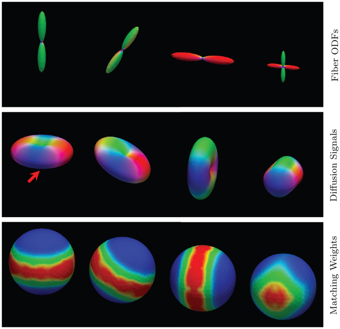
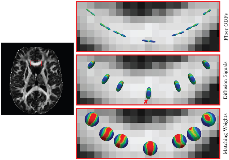
We first evaluated the performance of the proposed q-space patch matching. The results, shown in Fig. 6, indicate that the new patch matching scheme is robust to the variation of local fiber orientations. This allows XQ-NLM to use information from differentially oriented signal profiles for effective denoising. Fig. 7, generated using real data, confirms the observations from Fig. 6 and demonstrates that XQ-NLM is capable of locating recurrent information in curved white matter structures.
Fig. 6.
q-Space Patch Matching – Synthetic Data. Fiber ODFs are shown in the top row for reference. The middle row shows the profiles of the diffusion signals. Patch matching is performed using the point marked by the red arrow as the reference. The bottom row shows the matching results of signal profiles in different orientations. Warm colors indicate greater agreement, cool colors indicate otherwise. (For interpretation of the references to color in this figure legend, the reader is referred to the web version of this article.)
Fig. 7.
q-Space Patch Matching – Real Data. Similar to Fig. 6, but showing the results in the genu of the corpus callosum of a real dataset.
3.3.2. Synthetic data
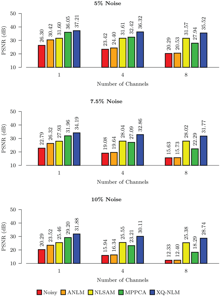
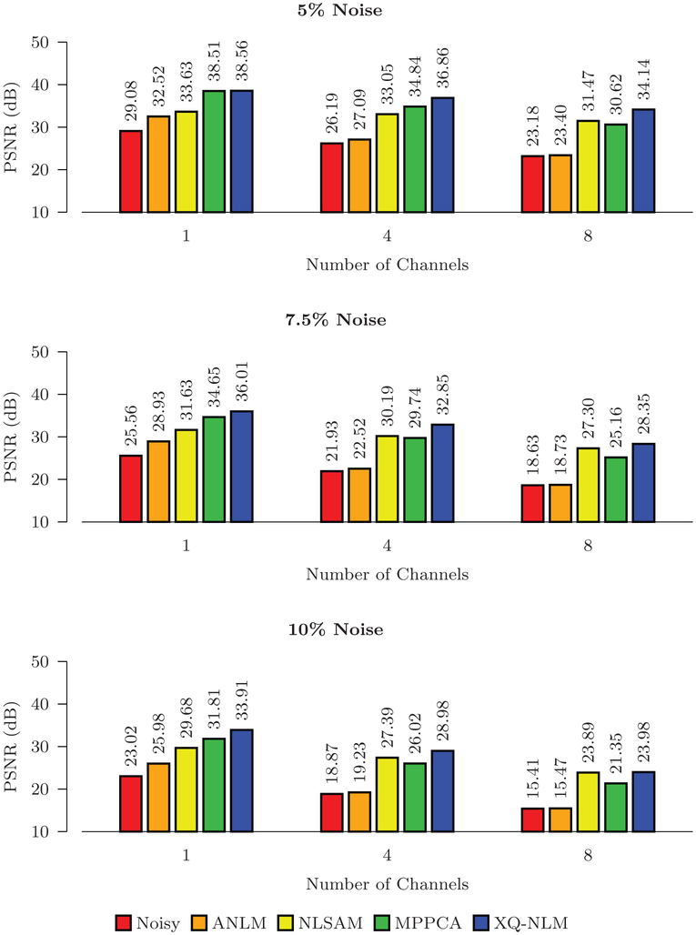
The PSNR results shown in Figs. 8 and 9 indicate that all methods improve the PSNR, but XQ-NLM performs best for all noise levels. MPPCA outperforms NLSAM when the number of channels is small. With the increase of noise level and number of channels, the performance of MPPCA drops dramatically and performs worse than NLSAM. Compared with NLSAM, the second best method, the largest improvement given by XQ-NLM is 6.42 dB in the case of 10% stationary Rician noise.
Fig. 8.
PSNR Comparison – Stationary Noise. Quantitative evaluation of denoising performance using synthetic data with spatially stationary noise.
Fig. 9.
PSNR Comparison – Non-Stationary Noise. Quantitative evaluation of denoising performance using synthetic data with spatially non-stationary noise.
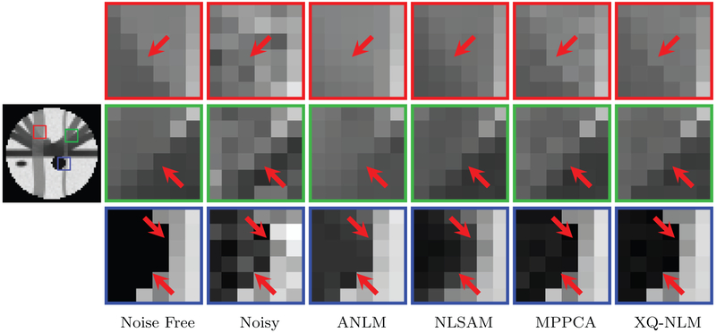
The denoised DW images, shown in Fig. 10, indicate that XQ-NLM is able to preserve sharp edges and effectively remove noise, thanks to the robust q-space patch matching mechanism, as demonstrated in Fig. 6. In contrast, ANLM and NLSAM blur edges and MPPCA is unable to sufficiently remove noise.
Fig. 10.
DW Images – Synthetic Data. Synthetic data (b = 1000 s/mm2) with 5% 4-channel spatially non-stationary nc-χ noise was used in the evaluation.
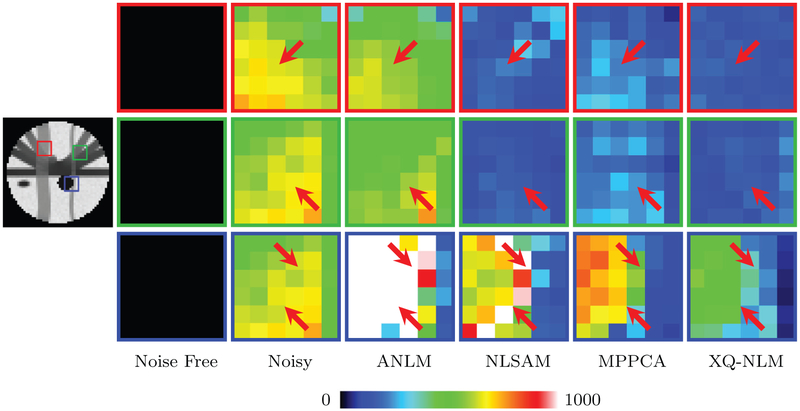
For better comparison, we computed the RMSE map of a denoised dataset with respect to the ground truth. The results, shown in Fig. 11, indicate that, compared with the baseline methods, XQ-NLM significantly reduces the RMSE. The improvement is especially apparent at the boundaries, compared with ANLM. NLSAM slightly improves the results, but is still problematic at boundaries. MP-PCA performs better than ANLM and NLSAM for edges, but fails to remove noise sufficiently. Overall, XQ-NLM yields superior performance with edge-preserving denoising.
Fig. 11.
RMSE Maps. Similar to Fig. 10, but showing RMSE maps. The color bar is capped at 1000, which is 10% of the maximum intensity value. (For interpretation of the references to color in this figure legend, the reader is referred to the web version of this article.)
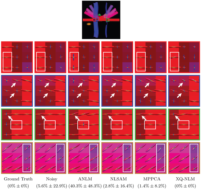
The ODFs, shown in Fig. 12, indicate that XQ-NLM gives results that are very close to the ground truth. In contrast, ANLM, NLSAM and MPPCA lead to incorrect results, as marked by the white arrows. When the smoothing effect is strong, as in ANLM, spurious peaks are more likely to occur at the boundaries. From the results given by ANLM in Fig. 12, we can observe that spurious peaks are introduced to single direction ODFs. These incorrect peaks are introduced from the neighboring two-direction ODFs due to boundary smoothing, as can be observed from Fig. 10. The PFFD means and standard deviations computed for the ROIs shown in Fig. 12 confirm that all fiber peaks are successfully recovered after denoising by XQ-NLM. MPPCA and NLSAM reduce PFFD but are still imperfect. ANLM induces spurious peaks and increases PFFD.
Fig. 12.
Fiber ODFs – Synthetic Data. White matter fiber ODFs for synthetic data. The PFFD means and standard deviations for the marked regions are shown at the bottom.
3.3.3. Repeated-acquisition data
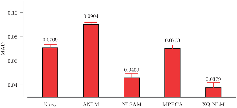
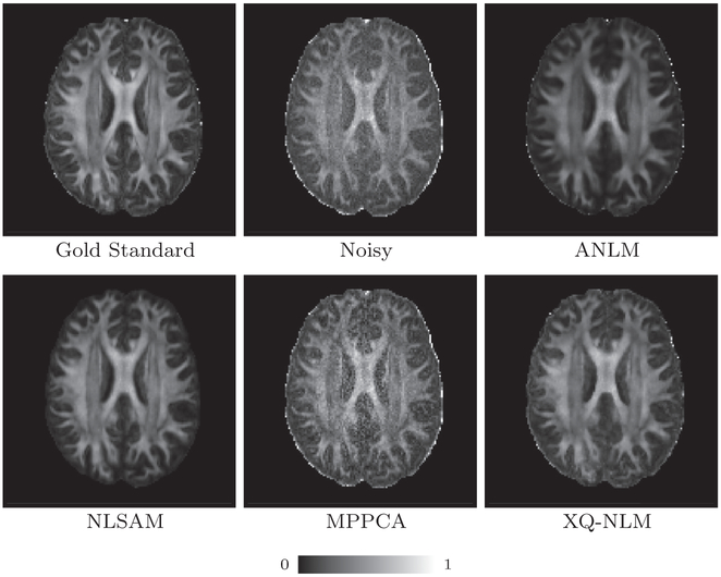
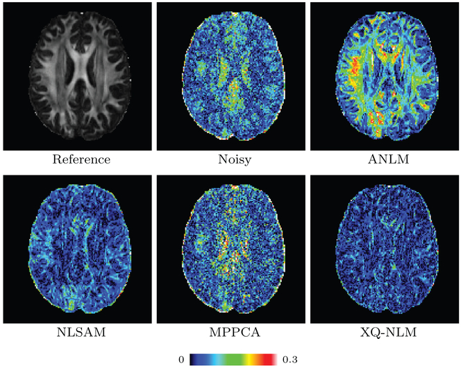
Fig. 13 indicates that XQ-NLM gives the lowest mean GFA MAD among the compared methods. Fig. 14 shows the GFA images of one randomly selected dataset. XQ-NLM gives a sharper GFA image with preserved details even in the cortical regions. The corresponding GFA AD maps, shown in Fig. 15, indicate that XQ-NLM gives on overall the lowest AD values, further confirming the advantages of XQ-NLM. The superior performance of XQ-NLM can be attributed to the fact that XQ-NLM is able to preserve edges while effectively remove noise. ANLM and NLSAM over-smooth and MP-PCA under-smooths the data, causing the GFA estimates to deviate from the true values.
Fig. 13.
GFA MAD. Means and standard deviations of the MAD values of the GFA images given by the different methods.
Fig. 14.
GFA Images. GFA images of one randomly selected dataset.
Fig. 15.
GFA AD Maps. Gold standard GFA image and the AD maps of Fig. 14.
3.3.4. Multi-shell HCP data
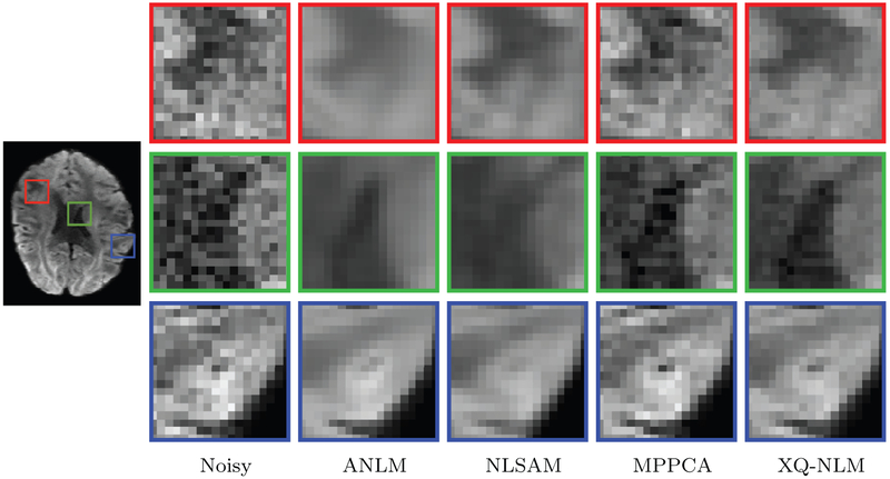
The results shown in Fig. 16 indicate that XQ-NLM yields markedly improved edge-preserving results in the cortical regions compared with ANLM, NLSAM, and MPPCA, especially at boundaries.
Fig. 16.
DW Images – HCP Data. DW images of the real data (b = 1000 s/mm2) denoised by various methods.
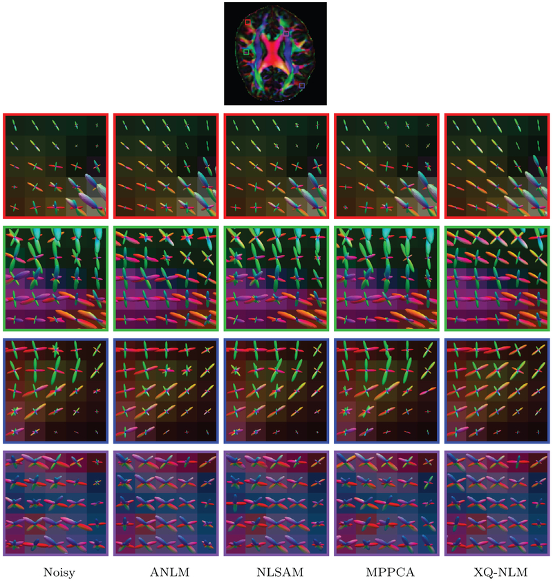
The influence of denoising on ODFs can be seen in Fig. 17. We can observe that XQ-NLM yields cleaner results with less spurious peaks. This improvement is essential for correctly tracing the axonal directions.
Fig. 17.
Fiber ODFs – HCP Data. White matter fiber ODFs in various regions.
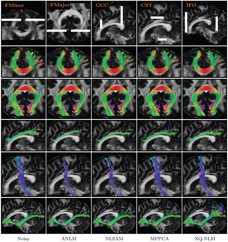
Finally, the tract bundles described in Table 1 were extracted for evaluation. The results, shown in Fig. 18, indicate that XQ-NLM gives smooth and rich tracts. In contrast, the tracts given by ANLM is over-smoothed and a significant number of tracts are missing. The noisy data and the data denoised by NLSAM and MPPCA give spurious tracts.
Table 1.
Tract bundles used for evaluation.
| Bundle | Description |
|---|---|
| FMinor | The frontal projection of the corpus callosum (i.e., forceps minor) |
| FMajor | The occipital projection of the corpus callosum (i.e., forceps major) |
| GCC | Genu of corpus callosum |
| CST | Corticospinal tract |
| IFO | Inferior fronto-occipital fasciculus |
Fig. 18.
Tract Bundles. Tract bundles given by the noisy data and denoised data generated using various methods.
4. Discussion
4.1. Factors contributing to the effectiveness of XQ-NLM
XQ-NLM demonstrates superb denoising and edge-preserving performance, which can be attributed mainly to the following factors:
Patch matching in q-space allows information from curved structures to be used for denoising. This dramatically increases the effective sample size and improves the chance of finding matching information.
NLM can be seen as kernel regression in patch space (Yap et al., 2014) and large kernel bandwidths are known to introduce bias (Silverman, 1998). The increase in sample size allows XQ-NLM to utilize a tighter matching criterion, i.e., smaller kernel band-widths, so that estimation bias can be reduced.
The diffusion signal profile captured in each voxel is in general smooth with less abrupt changes. This again improves effective sample size because sharp changes generally imply structural peculiarity and hence greater challenges in finding matching information.
Diffusion signal profiles have simpler shapes. This implies greater recurrence in signal patterns and hence more effective NLM denoising with lesser artifacts caused by the rare patch effect (Duval et al., 2011; Deledalle et al., 2012; Salmon and Strozecki, 2012).
4.2. Mitigating noise-induced bias
Unlike Gaussian noise, the signal dependency of nc-χ noise complicates the analysis of the CMS. The noise floor resulting from nc-χ noise leads to biased diffusion model fitting and inaccurate signal averaging. This can be avoided by employing signal transformation techniques, such as the one described in Section 2.1.2. Alternatively, if phase images are available, real-valued diffusion data can be extracted based on the approach described in Eichner et al. (2015). Essentially, the method eliminates shot-to-shot phase variations of complex-valued diffusion data so that real-valued signals with zero-mean Gaussian noise can be extracted.
4.3. Computational efficiency
We compared the computational times of the different methods using the repeated-acquisition data described in Section 3.1.2. Only one of the 25 datasets was used in this evaluation. XQ-NLM and ANLM were implemented using C++ based on the Insight Segmentation and Registration Toolkit (ITK).2 MP-PCA3 and NLSAM4 were compiled from source code. The speed was evaluated using a computer equipped with a four-core 2.9 GHz Intel Core i7 CPU. The results, shown in Table 2, indicate that XQ-NLM, while slower than MP-PCA and ANLM, is faster than NLSAM. The speed of XQ-NLM can be improved by using preselection strategies (Coupé et al., 2008) to quickly discard irrelevant patches so that they are not involved in the computation.
Table 2.
Comparison of computation times.
| ANLM | NLSAM | MPPCA | XQ-NLM | |
|---|---|---|---|---|
| Time (mins) | 33.2 | 332.2 | 3.5 | 115.5 |
4.4. Future directions
In DMRI, patch-based methods have a wide range of applications, including denoising (Wiest-Daesslé et al., 2007, 2008; Descoteaux et al., 2008; Yap et al., 2014), atlas building (Saghafi et al., 2017; Kim et al., 2017; Yang et al., 2017), fiber orientation estimation (Chen et al., 2016b; Ye et al., 2016), resolution enhancement (Chen et al., 2018), statistical group comparison (Chen et al., 2015), etc. Our x – q space patch matching strategy can be extended for these applications to better leverage the directional nature of DMRI data for performance improvements.
5. Conclusion
In this paper, we have proposed an improved NLM algorithm that caters to the spatio-angular characteristics of DMRI data. Our method, called XQ-NLM, performs patch matching in x – q space, allowing information from highly curved white matter structures to be used for effective noise removal. Extensive experiments demonstrate that XQ-NLM improves the SNR of DW images, preserves structural details, and reduces spurious fiber peaks that result from noise.
Acknowledgments
This work was supported in part by NIH grants (NS093842, EB022880, EB006733, EB009634, AG041721, MH100217, and AA012388). Data were provided in part by the Human Connectome Project, WU-Minn Consortium (Principal Investigators: David Van Essen and Kamil Ugurbil; 1U54MH091657) funded by the 16 NIH Institutes and Centers that support the NIH Blueprint for Neuro-science Research; and by the McDonnell Center for Systems Neuroscience at Washington University.
☆
Conflict of interest: There are no conflicts of interest.
References
- Aganj I, Lenglet C, Sapiro G, Yacoub E, Ugurbil K, Harel N, 2010. Reconstruction of the orientation distribution function in single-and multiple-shell q-ball imaging within constant solid angle. Magn. Reson. Med 64 (2), 554–566. [DOI] [PMC free article] [PubMed] [Google Scholar]
- Aja-Fernández S, Vegas-Sánchez-Ferrero G, 2016. Statistical Analysis of Noise in MRI. Springer. [Google Scholar]
- Aja-Fernández S, Vegas-Sánchez-Ferrero G, Tristán-Vega A, 2014. Noise estimation in parallel MRI: GRAPPA and SENSE. Magn. Reson. Imaging 32 (3), 281–290. [DOI] [PubMed] [Google Scholar]
- Andersson JL, Sotiropoulos SN, 2016. An integrated approach to correction for off-resonance effects and subject movement in diffusion MR imaging. NeuroImage 125, 1063–1078. [DOI] [PMC free article] [PubMed] [Google Scholar]
- Becker S, Tabelow K, Mohammadi S, Weiskopf N, Polzehl J, 2014. Adaptive smoothing of multi-shell diffusion weighted magnetic resonance data by msPOAS. NeuroImage 95, 90–105. [DOI] [PMC free article] [PubMed] [Google Scholar]
- Becker S, Tabelow K, Voss HU, Anwander A, Heidemann RM, Polzehl J, 2012. Position-orientation adaptive smoothing of diffusion weighted magnetic resonance data (POAS). Med. Image Anal 16 (6), 1142–1155. [DOI] [PubMed] [Google Scholar]
- Buades A, Coll B, Morel J-M, 2005. A review of image denoising algorithms, with a new one. Multiscale Model. Simul 4 (2), 490–530. [Google Scholar]
- Caruyer E, Daducci A, Descoteaux M, Houde J-C, Thiran J-P, Verma R, 2014. Phantomas: a flexible software library to simulate diffusion MR phantoms. Annual Meeting of the International Society for Magnetic Resonance in Medicine (ISMRM). [Google Scholar]
- Chen G, Dong B, Zhang Y, Lin W, Shen D, Yap P-T, 2018. Angular upsampling in infant diffusion MRI using neighborhood matching in x – q space. Front. Neuroinform 12, 57. [DOI] [PMC free article] [PubMed] [Google Scholar]
- Chen G, Wu Y, Shen D, Yap P-T, 2016a. XQ-NLM: denoising diffusion MRI data via x – q space non-local patch matching In: Medical Image Computing and Computer-Assisted Intervention (MICCAI). Springer, pp. 587–595. [DOI] [PMC free article] [PubMed] [Google Scholar]
- Chen G, Zhang J, Zhang Y, Dong B, Shen D, Yap P-T, 2019. Multi-channel framelet denoising of diffusion-weighted images. PLOS ONE. (In Press). [DOI] [PMC free article] [PubMed] [Google Scholar]
- Chen G, Zhang P, Li K, Wee C-Y, Wu Y, Shen D, Yap P-T, 2015. Block-based statistics for robust non-parametric morphometry. In: International Workshop on Patch-based Techniques in Medical Imaging Springer International Publishing, pp. 62–70. [DOI] [PMC free article] [PubMed] [Google Scholar]
- Chen G, Zhang P, Li K, Wee C-Y, Wu Y, Shen D, Yap P-T, 2016b. Improving estimation of fiber orientations in diffusion MRI using inter-subject information sharing. Sci. Rep 6, 37847. [DOI] [PMC free article] [PubMed] [Google Scholar]
- Chen G, Zhang P, Wu Y, Shen D, Yap P-T, 2016c. Denoising magnetic resonance images using collaborative non-local means. Neurocomputing 177, 215–227. [DOI] [PMC free article] [PubMed] [Google Scholar]
- Constantinides CD, Atalar E, McVeigh ER, 1997. Signal-to-noise measurements in magnitude images from NMR phased arrays. Magn. Reson. Med 38 (5), 852–857. [DOI] [PMC free article] [PubMed] [Google Scholar]
- Coupé P, Yger P, Prima S, Hellier P, Kervrann C, Barillot C, 2008. An optimized blockwise nonlocal means denoising filter for 3-D magnetic resonance images. IEEE Trans. Med. Imaging 27 (4), 425–441. [DOI] [PMC free article] [PubMed] [Google Scholar]
- Daducci A, Van De Ville D, Thiran J-P, Wiaux Y, 2014. Sparse regularization for fiber ODF reconstruction: from the suboptimality of l2, and l1 priors to l0. Med. Image Anal 18 (6), 820–833. [DOI] [PubMed] [Google Scholar]
- Deledalle C-A, Duval V, Salmon J, 2012. Non-local methods with shape-adaptive patches (NLM-SAP). J. Math. Imaging Vis 43 (2), 103–120. [Google Scholar]
- Descoteaux M, Wiest-Daesslé N, Prima S, Barillot C, Deriche R, 2008. Impact of Rician adapted non-local means filtering on HARDI In: Medical Image Computing and Computer-Assisted Intervention (MICCAI). Springer, pp. 122–130. [DOI] [PubMed] [Google Scholar]
- Dietrich O, Raya JG, Reeder SB, Ingrisch M, Reiser MF, Schoenberg SO, 2008. Influence of multichannel combination, parallel imaging and other reconstruction techniques on MRI noise characteristics. Magn Reson Imaging 26 (6), 754–762. [DOI] [PubMed] [Google Scholar]
- Duval V, Aujol J-F, Gousseau Y, 2011. A bias-variance approach for the nonlocal means. SIAM J. Imaging Sci 4 (2), 760–788. [Google Scholar]
- Eichner C, Cauley SF, Cohen-Adad J, Möller HE, Turner R, Setsompop K, Wald LL, 2015. Real diffusion-weighted MRI enabling true signal averaging and increased diffusion contrast. NeuroImage 122, 373–384. [DOI] [PMC free article] [PubMed] [Google Scholar]
- Garyfallidis E, Brett M, Amirbekian B, Rokem A, Van Der Walt S, Descoteaux M, Nimmo-Smith I, 2014. Dipy, a library for the analysis of diffusion MRI data. Front. Neuroinform 8, 8. [DOI] [PMC free article] [PubMed] [Google Scholar]
- Griswold MA, Jakob PM, Heidemann RM, Nittka M, Jellus V, Wang J, Kiefer B, Haase A, 2002. Generalized autocalibrating partially parallel acquisitions (GRAPPA). Magn Reson Med 47 (6), 1202–1210. [DOI] [PubMed] [Google Scholar]
- Gudbjartsson H, Patz S, 1995. The Rician distribution of noisy MRI data. Magn. Reson. Med 34 (6), 910–914. [DOI] [PMC free article] [PubMed] [Google Scholar]
- Johansen-Berg H, Behrens TE, 2013. Diffusion MRI: From Quantitative Measurement to in vivo Neuroanatomy. Academic Press. [Google Scholar]
- Kim J, Chen G, Lin W, Yap P-T, Shen D, 2017. Graph-constrained sparse construction of longitudinal diffusion-weighted infant atlases In: Medical Image Computing and Computer-Assisted Intervention (MICCAI). Springer, pp. 49–56. [DOI] [PMC free article] [PubMed] [Google Scholar]
- Koay CG, Basser PJ, 2006. Analytically exact correction scheme for signal extraction from noisy magnitude MR signals. J. Magn. Reson 179 (2), 317–322. [DOI] [PubMed] [Google Scholar]
- Koay CG, Özarslan E, Basser PJ, 2009a. A signal transformational framework for breaking the noise floor and its applications in MRI. J. Magn. Reson 197 (2), 108–119. [DOI] [PMC free article] [PubMed] [Google Scholar]
- Koay CG, Özarslan E, Pierpaoli C, 2009b. Probabilistic identification and estimation of noise (PIESNO): a self-consistent approach and its applications in MRI. J. Magn. Reson 199 (1), 94–103. [DOI] [PMC free article] [PubMed] [Google Scholar]
- Lam F, Babacan SD, Haldar JP, Weiner MW, Schuff N, Liang Z-P, 2014. Denoising diffusion-weighted magnitude MR images using rank and edge constraints. Magn. Reson. Med 71 (3), 1272–1284. [DOI] [PMC free article] [PubMed] [Google Scholar]
- Manjón JV, Coupé P, Concha L, Buades A, Collins DL, Robles M, 2013. Diffusion weighted image denoising using overcomplete local PCA. PLOS ONE 8 (9), e73021. [DOI] [PMC free article] [PubMed] [Google Scholar]
- Manjón JV, Coupé P, Martí-Bonmatí L, Collins DL, Robles M, 2010. Adaptive non-local means denoising of MR images with spatially varying noise levels. J. Magn. Reson. Imaging 31 (1), 192–203. [DOI] [PubMed] [Google Scholar]
- Mori S, Crain BJ, Chacko V, Van Zijl P, 1999. Three-dimensional tracking of axonal projections in the brain by magnetic resonance imaging. Ann. Neurol 45 (2), 265–269. [DOI] [PubMed] [Google Scholar]
- Prima S, Commowick O, 2013. Using bilateral symmetry to improve non-local means denoising of MR brain images. In: International Symposium on Biomedical Imaging (ISBI) IEEE, pp. 1231–1234. [Google Scholar]
- Pruessmann KP, Weiger M, Scheidegger MB, Boesiger P, et al. , 1999. SENSE: sensitivity encoding for fast MRI. Magn. Reson. Med 42 (5), 952–962. [PubMed] [Google Scholar]
- Saghafi B, Kim J, Chen G, Shi F, Lin W, Yap P-T, Shen D, 2017. Spatio-angular consistent construction of neonatal diffusion MRI atlases. Hum. Brain Mapp 38 (6), 3175–3189. [DOI] [PMC free article] [PubMed] [Google Scholar]
- Salmon J, Strozecki Y, 2012. Patch reprojections for non-local methods. Signal Process. 92 (2), 477–489. [Google Scholar]
- Silverman B, 1998. Density Estimation for Statistics and Data Analysis Monographs on Statistics and Applied Probablilty. Chapman and Hall. [Google Scholar]
- Sotiropoulos SN, Jbabdi S, Xu J, Andersson JL, Moeller S, Auerbach EJ, Glasser MF, Hernandez M, Sapiro G, Jenkinson M, et al. , 2013. Advances in diffusion MRI acquisition and processing in the human connectome project. NeuroImage 80, 125–143. [DOI] [PMC free article] [PubMed] [Google Scholar]
- St-Jean S, Coupé P, Descoteaux M, 2016. Non local spatial and angular matching: enabling higher spatial resolution diffusion MRI datasets through adaptive denoising. Med. Image Anal. 32, 115–130. [DOI] [PubMed] [Google Scholar]
- Stieltjes B, Kaufmann WE, van Zijl PC, Fredericksen K, Pearlson GD, Solaiyappan M, Mori S, 2001. Diffusion tensor imaging and axonal tracking in the human brainstem. NeuroImage 14 (3), 723–735. [DOI] [PubMed] [Google Scholar]
- Tuch DS, 2004. Q-ball imaging. Magn. Reson. Med. 52 (6), 1358–1372. [DOI] [PubMed] [Google Scholar]
- Van Essen DC, Smith SM, Barch DM, Behrens TE, Yacoub E, Ugurbil K, Consortium, W.-M.H., et al. , 2013. The WU-Minn human connectome project: an overview. NeuroImage 80, 62–79. [DOI] [PMC free article] [PubMed] [Google Scholar]
- Varadarajan D, Haldar JP, 2015. A majorize-minimize framework for Rician and non-central Chi MR images. IEEE Trans. Med. Imaging 34 (10), 2191–2202. [DOI] [PMC free article] [PubMed] [Google Scholar]
- Veraart J, Novikov DS, Christiaens D, Ades-Aron B, Sijbers J, Fieremans E, 2016. Denoising of diffusion MRI using random matrix theory. NeuroImage 142, 394–406. [DOI] [PMC free article] [PubMed] [Google Scholar]
- Veraart J, Rajan J, Peeters RR, Leemans A, Sunaert S, Sijbers J, 2013. Comprehensive framework for accurate diffusion MRI parameter estimation. Magn. Reson. Med 70 (4), 972–984. [DOI] [PubMed] [Google Scholar]
- Wakana S, Caprihan A, Panzenboeck MM, Fallon JH, Perry M, Gollub RL, Hua K, Zhang J, Jiang H, Dubey P, et al. , 2007. Reproducibility of quantitative tractography methods applied to cerebral white matter. NeuroImage 36 (3), 630–644. [DOI] [PMC free article] [PubMed] [Google Scholar]
- Wessel P, Smith WH, 2001. The generic mapping tools. [Google Scholar]
- Wiest-Daesslé N, Prima S, Coupé P, Morrissey SP, Barillot C, 2007. Non-local means variants for denoising of diffusion-weighted and diffusion tensor MRI In: Medical Image Computing and Computer-Assisted Intervention (MICCAI). Springer, pp. 344–351. [DOI] [PMC free article] [PubMed] [Google Scholar]
- Wiest-Daesslé N, Prima S, Coupé P, Morrissey SP, Barillot C, 2008. Rician noise removal by non-local means filtering for low signal-to-noise ratio MRI: applications to DT-MRI In: Medical Image Computing and Computer-Assisted Intervention (MICCAI). Springer, pp. 171–179. [DOI] [PMC free article] [PubMed] [Google Scholar]
- Yang Z, Chen G, Shen D, Yap P-T, 2017. Robust fusion of diffusion MRI data for template construction. Sci. Rep 7 (1), 12950. [DOI] [PMC free article] [PubMed] [Google Scholar]
- Yap P-T, An H, Chen Y, Shen D, 2014. Uncertainty estimation in diffusion MRI using the nonlocal bootstrap. IEEE Trans. Med. Imaging 33 (8), 1627–1640. [DOI] [PMC free article] [PubMed] [Google Scholar]
- Yap P-T, Jiang X, Kot AC, 2010. Two-dimensional polar harmonic transforms for invariant image representation. IEEE Trans. Pattern Anal. Mach. Intell 32 (7), 1259–1270. [DOI] [PubMed] [Google Scholar]
- Yap PT, Zhang Y, Shen D, 2016. Multi-tissue decomposition of diffusion MRI signals via l0 sparse-group estimation. IEEE Trans. Image Process. 25 (9), 4340–4353. [DOI] [PMC free article] [PubMed] [Google Scholar]
- Ye C, Zhuo J, Gullapalli RP, Prince JL, 2016. Estimation of fiber orientations using neighborhood information. Med. Image Anal 32, 243–256. [DOI] [PMC free article] [PubMed] [Google Scholar]


