Medical Image Synthesis with Deep Convolutional Adversarial Networks

Abstract

Medical imaging plays a critical role in various clinical applications. However, due to multiple considerations such as cost and radiation dose, the acquisition of certain image modalities may be limited. Thus, medical image synthesis can be of great benefit by estimating a desired imaging modality without incurring an actual scan. In this paper, we propose a generative adversarial approach to address this challenging problem. Specifically, we train a fully convolutional network (FCN) to generate a target image given a source image. To better model a nonlinear mapping from source to target and to produce more realistic target images, we propose to use the adversarial learning strategy to better model the FCN. Moreover, the FCN is designed to incorporate an image-gradient-difference-based loss function to avoid generating blurry target images. Long-term residual unit is also explored to help the training of the network. We further apply Auto-Context Model to implement a context-aware deep convolutional adversarial network. Experimental results show that our method is accurate and robust for synthesizing target images from the corresponding source images. In particular, we evaluate our method on three datasets, to address the tasks of generating CT from MRI and generating 7T MRI from 3T MRI images. Our method outperforms the state-of-the-art methods under comparison in all datasets and tasks.

I. Introduction

MEDICAL imaging is crucial in the diagnosis and treatment of different illness. Usually more than one imaging modalities are involved in the clinical decision making because different modalities often provide complementary insights. Computer tomography (CT), for example, has the advantage of providing electron density and physical density of the tissues, which is indispensable for dosage planning in radiotherapy treatment of cancer patients. However, CT suffers from the disadvantage of lacking good contrast in soft tissues. The radiation exposure during acquisition may also increase the risk of secondary cancer especially for the young patients. Magnetic resonance imaging (MRI), on the other hand, gives very good contrast of soft tissues. Compared to CT, MRI is also much safer and does not involve any radiation; but it is much more costly than CT and does not have the density information that is needed for radiation therapy planning or PET image reconstruction [1].

In a second example, the acquired images cannot well depict rich details of anatomical structures and abnormality. For instance, it is difficult to delineate small brain structures such as the hippocampus in 3T MRI images because of the limited spatial resolution [2]–[4]. 7T MRI, on the contrary, provides much better image quality than 3T MRI by revealing certain texture information within the hippocampus. This allows better observation towards the anatomy and thus contributes to better utilization of the imaging data. Yet 7T MRI is much more expensive and not widely accessible to the public in the world.

The above observations reflect a general dilemma, where a certain modality is desired but infeasible to acquire in practice. To this end, a system being able to synthesize images-of-interest from different sources, e.g., image modalities and acquisition protocols, can be of great benefit. It may provide the highly demanded imaging data for certain clinical usage, without incurring in additional cost/risk of performing a real acquisition.

However, medical image synthesis is very challenging to solve directly since the mapping from the source image to the target image (or its inverse) is usually of high dimensionality and ill-posed [5]–[7]. As shown in Fig. 1(a) and (b), CT and MRI data of the same subject have quite different appearances. And thus the mapping from MRI to CT has to be highly nonlinear in order to bridge the significant appearance gap between the two modalities, which requires a lot of effort to model. Shown in Fig. 1(c), the 7T MRI has much higher resolution and much clearer contrast compared to the 3T MRI, which makes the mapping from 3T MRI to 7T MRI very challenging.

Fig. 1.

Three pairs of corresponding source (left) and target (right) images from the same subjects. (a) shows a pair of MRI/CT brain images; (b) shows a pair of MRI/CT pelvic images; (c) shows a pair of 3T/7T brain MRI.

Recently, many researches have focused on estimating one modality image from another and proposed many methods to address this challenge [8]–[12]. Berker et al. [8], for example, proposed to treat the MRI-to-CT problem as a segmentation task by segmenting MRI images into different tissue classes and then assigning each class with a known attenuation property. This method highly depends on the segmentation accuracy and always needs manual work for the accuracy of the results. On the other hand, atlas-based methods have also been used in the literature. In [10], the authors proposed to register an atlas to the new subject’s source image and then warp the corresponding target image of the atlas as the estimated target image.

In [13], the authors proposed an extension of the well known Label Propagation (LP) segmentation algorithm. They called it Modality Propagation and provided a generalization of LP allowing to work with continuous data instead of only categorical segmentation labels. Similarly, in [14], the authors proposed an information propagation scheme, here for a given source patch, the system looks for similar patches in the source dataset, and constructs the target image based on their corresponding target (which is known in the training set). However, the accuracies of these atlas-based methods are highly sensible to the registration accuracies.

Besides, learning-based methods have also been explored to model a nonlinear mapping from source image to target image, to alleviate some of the previous drawbacks [15]–[24]. For instance, Jog et al. [16] learned a nonlinear regression with random forest to carry out cross-modality synthesis of high resolution images from low resolution scans. Huynh et al. [18] presented an approach to synthesize CT from MRI using random forest as well. Unsupervised methods have also been used. In [25] for example, the authors proposed a framework where for each voxel in the source image, a set of target candidate values was generated by a nearest neighbor search in the training set of target images. Note that since there is no paired data, they need a similarity measure that is somewhat robust to changes in modality, in this case they use mutual information. Then, they select the best candidates by maximizing a global energy function that takes into account the mutual information between the source and target, and also the spatial consistency in the generated target. These methods often have to first represent the source image by features and then map them to generate the target image. Thus, the performances of these methods are bounded to the manually engineered features as well as the quality of the representation of the source image based on the extracted features.

Nowadays, deep learning has become very popular in computer vision and medical image analysis, achieving state-of-the-art results in both fields without the need of hand-crafted features [26]–[29]. In the particular case of image synthesis, Dong et al. [30] proposed to use Convolutional Neural Networks (CNNs) for single image super-resolution. Kim et al. [31] further improved the super-resolution algorithm by proposing a recursive CNN which can boost performance without increasing parametric complexity. Li et al. [32] applied a similar deep learning model to estimate the missing PET image from the MRI data of the same subject. Huang et al. [33] proposed to simultaneously conduct super-resolution and cross-modality medical image synthesis by the weakly-supervised joint convolutional sparse coding.

One potential problem of CNN is that it tends to neglect neighborhood information in the predicted target image, especially when the input size is small. To overcome this, Fully Convolutional Networks (FCNs), which can preserve structural information, have been utilized for image synthesis [33], [34]. Typically, the L2 distance between the predicted target image and the ground truth is used as the loss function to train the CNNs and FCNs, which tends to yield blurry target images especially in multi-modal distributions [35]. Minimizing the L2 loss is equivalent to maximizing the peak signal-to-noise rate (PSNR); however, as it has been pointed out in [36], a higher PSNR does not necessarily provide a perceptually better result.

To address the above mentioned drawbacks, in this paper, we propose to learn the nonlinear mapping from source images to target images through the generative adversarial framework in order to produce more realistic target images. Specifically, we utilize the adversarial strategy to train a 3D FCN, which acts as the generator of realistic target images. An additional discriminator network is also trained simultaneously, which urges the generator’s output to be similar with the ground-truth target image perceptually. Inspired by [35] and with the aim of alleviating the intrinsic blurriness of the target image generated by FCN, we propose to utilize an additional term in the loss function based on image gradient difference. Besides, we also adopt residual learning for easy training of the network. Since the network is trained in a patch-to-patch manner and its receptive field is thus restricted, we are inspired by the Auto-Context Model (ACM) to concatenate several trained networks, such that the entire framework includes long-range visibility to image information and becomes context-aware. The proposed method is evaluated on three real datasets and two tasks (particularly, two datasets for the first task of MRI-to-CT estimation and another dataset for the task of 3T-to-7T estimation). Experimental results demonstrate that our method can effectively generate target images from the corresponding sources and also outperform the state-of-the-art methods under comparison.

A preliminary version of this work has been presented at a conference [37]. Herein, we (i) extend our method by introducing the long-term residual connection in the generator and verify its capability for the challenging 3T-to-7T imaging synthesis task, (ii) evaluate and further analyze the impact of the proposed image gradient difference loss function, (iii) include evaluation and analysis of the iterative auto-context refinement, (iv) analyze the convergence after applying the long-term residual connection, and (vi) include additional discussions that are not in the conference publication.

II. Methods

To address the above mentioned problems and challenges, we propose a deep convolutional adversarial network framework by adversarially training FCN as the generator and CNN as the discriminator. First, we propose a basic 3D FCN to estimate the target image from the corresponding source image. Note that we adopt 3D operations to better model the 3D spatial mapping and thus could solve the discontinuity problem across 2D slices, which often occurs when using the 2D CNN. Second, we utilize the adversarial learning strategy [38] for the designed network, where an additional discriminator network is modeled. The discriminator urges the generator’s output to be similar with the ground-truth target image perceptually. Our generator is featured by incorporating the image gradient difference into the loss function, with the goal of retaining the sharpness of the generated target image. We further explore the long-term residual unit to train the network. Moreover, we employ ACM to iteratively refine the output of the generator. At the testing stage, an input source image is first partitioned into overlapping patches, and, for each patch, the corresponding target is estimated by the generator. Then, all generated target patches are merged into a single image to complete the source-to-target synthesis by averaging the intensities of overlapping CT regions. In the following, we will describe in detail the GAN framework used in the source-to-target image synthesis.

A. Supervised Deep Convolutional Adversarial Network

As mentioned above, we propose a supervised deep convolutional adversarial framework, which is inspired by the recent popular generative adversarial networks (GAN) [38], to complete the source-to-target synthesis as shown in Fig. 2. The components in Fig. 2 will be introduced in the following paragraphs. Fully Convolutional Network (FCN) for Medical Image Synthesis: FCN is widely used for segmentation and reconstruction in both computer vision and medical image analysis fields [4], [34], [39]-[43], because it can preserve spatial information in local neighborhood of the image space and is also much faster compared to CNN at the testing stage. In this paper, we adopt FCN to implement the image generator. A typical 3D FCN (as shown in Fig. 3) is proposed to perform the medical image synthesis task. We use only the convolution operations without pooling, which would potentially lead to loss of resolution.

Fig. 2.

Architecture used in the deep convolutional adversarial setting for estimation of the synthetic target image.

Fig. 3.

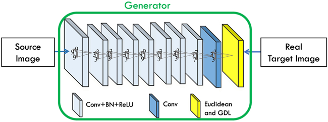
3D FCN architecture for estimating a target image from a source image.

As mentioned in the Introduction section, typically a Euclidean loss is used to train the model as shown in (1).

$$L_G(X,Y)={\Vert Y-G(X)\Vert }_2^2$$ (1)

where Y is the ground-truth target image, and G(X) is the generated target image from the source image X by the Generator network G.

Adversarial Learning:

To make the generated target images better perceptually, we propose to use adversarial learning to improve the performance of FCN.

GANs have achieved the state-of-the-art results in the field of image generation by producing very realistic images in an unsupervised setting [38], [44]. Inspired by the works in [35], [38], we propose the supervised GAN to synthesize medical images. Our networks include 1) the generator for estimating the target image and 2) the discriminator for distinguishing the real target image from the generated one, as shown in Fig. 2. The generator network G is an FCN as described above. The discriminator network D is a CNN, which estimates the probability of the input image being drawn from the distribution of real images. That is, D can classify an input image as “real” or “synthetic”.

Both networks are trained simultaneously, with D trying to correctly discriminate real and synthetic data, and G trying to produce realistic images that confuse D. Concretely, the loss function for D and G can be defined as:

$$L_D(X,Y)=L_{\mathit{BCE}}(D(Y),1)+L_{\mathit{BCE}}(D(G(X)),0)$$ (2)

where X is the source input image, Y is the corresponding target image, G(X) is the estimated image by the generator, and D (·) computes the probability of the input to be “real”. And, L_BCE is the binary cross entropy defined by (3).

$$L_{\mathit{BCE}}(\widehat{Y},Y)=-\sum _i{Y}_i\log \left({\widehat{Y}}_i\right)+(1-Y_i)\log \left(1-{\widehat{Y}}_i\right)$$ (3)

where Y represents the label of the input data and takes its values in {0, 1} (i.e., 0 for the generated image and 1 for the real one), and $\widehat{Y}$ is the predicted probability in [0, 1] that the discriminator assigns to the input of being drawn from the distribution of real images.

On the other hand, the loss term used to train G is defined as:

$$L_{G\_\mathit{ADV}}(X,Y)={\lambda }_1{L}_{\mathit{ADV}}(X)+{\lambda }_2{L}_G(X,Y)+{\lambda }_3{L}_{\mathit{GDL}}(Y,G(X))$$ (4)

Specifically, we minimize the binary cross entropy (“BCE”) between the decisions of D and the correct labels (“real” or “synthetic”), while the network G minimizes the binary cross entropy between the decisions by D and the wrong labels for the generated images. The loss of G incorporates the traditional term used for image synthesis in (1), as well as several more terms that will be detailed later. In general, D can distinguish between the real target data and the synthetic target data generated by G. At the same time, G aims to produce more realistic target images and to confuse D.

In the case of G, we use a loss function that includes an adversarial term (“ADV”) to fool D:

$$L_{\mathit{ADV}}(X)=L_{\mathit{BCE}}(D(G(X)),1)$$ (5)

The training of the two networks is performed in an alternating fashion. First, D is updated by taking a mini-batch of real target data and a mini-batch of generated target data (corresponding to the output of G). Then, G is updated by using another mini-batch of samples including sources and their corresponding ground-truth target images.

Image Gradient Difference Loss:

If we only take into account (5) only for the generator, the system would be able to generate images that are drawn from the distribution of the target data. We further incorporate the L2 loss term of (1) as a data fitting term in the loss of the generator, aiming at producing realistic images. Training the system with the above mentioned losses would be able to generate a target image from its corresponding source image. Furthermore, as the L2 loss may produce blurry images, we propose to use an image gradient difference loss (“GDL”) as an additional term. It is defined as:

$$\begin{gathered} L_{\mathit{GDL}}(Y,\widehat{Y})={\mid \mid \nabla Y_x\mid -\mid \nabla {\widehat{Y}}_x\mid \mid }^2 \\ +{\mid \mid \nabla Y_y\mid -\mid \nabla {\widehat{Y}}_y\mid \mid }^2 \\ +{\mid \mid \nabla Y_z\mid -\mid \nabla {\widehat{Y}}_z\mid \mid }^2 \end{gathered}$$ (6)

where Y is the ground-truth target image, and $\widehat{Y}$ is the estimated target by the generator network. This loss tries to minimize the difference of the magnitudes of the gradients between the ground-truth target image and the synthetic target image. In this way, the synthetic target image will try to keep the regions with strong gradients (i.e., edges) for an effective compensation of the L2 reconstruction term. By combining all losses above, the generator can thus be modeled to minimize the loss function shown in (4).

Architecture Details:

We show the architecture of our generator network G in Fig. 3, where the numbers indicate the filter sizes. This network takes a source image as the input, and tries to generate the corresponding target image. The architecture is designed with empirical knowledge from the widely-used FCN architectures. As the input size of our network is 32 × 32 × 32 and the output size is 16 × 16 × 16, we have to reduce the feature map sizes during the network inference. If we keep using 3 × 3 × 3 as the kernel size, we will have too many layers, which is challenging to both physical memory and optimization in training. Thus, we choose several big kernels to decrease the depth of the network in the generator. Our kernel size setting is empirical, and we believe that other possible configurations can also be used. Specifically, it has 9 layers containing convolution, batch normalization (BN) and ReLU operations. The kernel sizes are 9³, 3³, 3³, 3³, 9³, 3³, 3³, 7³, and 3³ respectively. The numbers of filters are 32, 32, 32, 64, 64, 64, 32, 32, and 1, respectively, for the individual layers. The last layer only includes 1 convolutional filter, and its output is considered as the estimated target image. Regarding the architecture, we avoid the use of pooling since it will reduce the spatial resolution of the feature maps. Considering the fact that the traditional convolution operations of the generator in Fig. 2 cannot guarantee a sufficiently effective receptive field [45], we adopt the dilated convolution as an alternative [46] so that we can achieve enough receptive field. The dilation for the first and last convolution layers of the generator in Fig. 2 are 1, and 2 for all the rest convolution layers.

The discriminator D is a typical CNN architecture including three stages of convolution, BN, ReLU and max pooling, followed by one convolutional layer and three fully connected layers where the first two use ReLU as activation functions and the last one uses sigmoid (whose output represents the likelihood that the input data is drawn from the distribution of real target image). The filter size is 3 × 3 × 3, the numbers of the filters are 32, 64, 128 and 256 for the convolutional layers, and the numbers of the output nodes in the fully connected layers are 512, 128 and 1.

B. Residual Learning for the Generator

CNN with residual connections has achieved promising results in many challenging generic image processing tasks [28], [47]. Residual connections, in principle, help bypass the nonlinear transformations with an identity mapping in the network and explicitly reformulates the layers as learning residuals with reference to the precedent layers [28]. Formally, the residual connection can be expressed as (7):

$$y=F(x,\{W_i\})+x,$$ (7)

where W_i are the convolutional filters in the bottleneck residual unit, and x and y are the input and output feature maps, respectively.

‘ResNet’ demonstrates that the residual connection benefits convergence when training a very deep CNN. The residual learning unit works on a local convolutional layer by transforming it to a bottleneck architecture. Since in some tasks, the source and target images (e.g., 3T-to-7T task) are largely similar, in this paper, we extend such a connection (bottleneck architecture) to skip the whole CNN (or FCN), instead of a single convolutional layer. With this long-term residual unit, the residual image is likely to be (or close to be) zero, making the network much easier to train. The long-term residual connection is illustrated as the solid-purple-line arrow in Fig. 4.

Fig. 4.

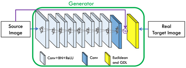
Generator architecture used in the GAN setting for estimation of synthetic target image. Note the solid-purple-line arrow from source image to the “plus” sign, which expresses the long-term residual connection.

For the 3T-to-7T synthesis task, it might be hard for very deep networks to produce accurate results since the model will require a very long-term memory [31]. This is due to the fact that the structure of the output is very similar to the structure of the input, and the required memory might be difficult to model during the training because of vanishing gradient issues and the large number of layers. As introduced in the above paragraphs, residual learning can help to alleviate this issue by learning a residual map in the last layer [28], [47]. This is accomplished by adding a skip connection from the input to the final layer and then performing an element-wise addition. In Fig. 4, we show this architecture. It is worth mentioning that this longterm residual unit only makes sense for tasks where the input is highly correlated to the output, such as 3T-to-7T synthesis, super resolution, denoising and so on. For that reason, we only use this method for the 3T-to-7T synthesis task in this paper.

C. Auto-Context Model (ACM) for Refinement

Since our work is patch-based, the context information available for each training sample is limited inside the patch. This obviously affects the modeling capacity of our network. One remedy to enlarge the context during training is by using ACM, which is commonly used in the task of semantic segmentation [48]. The idea is to train several classifiers iteratively, where each classifier is trained not only with the feature data of original image(s) but also with the probability map outputted by the previous classifier. Note that the output of the previous classifier gives additional context information for the subsequent classifier to use. At testing time, the input will be processed for each classifier one after the other, concatenating the probability map to the initial input.

In this work, we show that the ACM can also be applied successfully to the deep learning based regression tasks. In particular, we adopt the ACM to iteratively refine the generated results, making our GAN context-aware. To this end, we iteratively train several GANs that take inputs from both early synthetic target patches and source patches. These patches are then concatenated as a second channel with the source patches, which are both input for training of the next GAN. An illustration of this scheme is shown in Fig. 5. It is worth noting that the architectures of the GANs we use for ACM are exactly the same as shown in Fig. 2. The only difference is about the input to the generator, which concatenates the source MRI patch and the synthetic target patch since the 1st iteration of ACM. We keep same sizes of the input patches throughout the ACM based refinement. Since the context information is extracted from the whole previously-estimated target image, they can encode information that is not available within the initial input image patch.

Fig. 5.

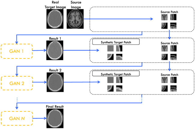
Proposed architecture for ACM with GAN.

III. Experiments and Results

We use three datasets to test our proposed method in two different tasks. First, we estimate CT images from its corresponding MRI data for both pelvic and brain datasets. Second, we estimate 7T MRI data from its corresponding 3T MRI data. We will describe the experiments and the results of these two tasks separately.

A. Experiments on MR-to-CT Synthesis

1. The brain dataset was acquired from 16 subjects with both MRI and CT scans in the Alzheimer’s Disease Neuroimaging Initiative (ADNI) database (see www.adni-info.org for details). The MR images were acquired using a Siemens Triotim scanner, with the voxel size 1.2 × 1.2 × 1 mm³ , TE 2.95 ms, TR 2300 ms, and flip angle 9°. The CT images, with the voxel size 0.59 × 0.59 × 3 mm³, were acquired on a Siemens Somatom scanner. A typical example of preprocessed CT and MR images is given in Fig. 1.

2. Our pelvic dataset consists of 22 subjects, each with MR and CT images. The spacings of CT and MR images are 1.172 × 1.172 × 1 mm³ and 1 × 1 × 1 mm³, respectively. In the training stage, we rigidly align the CT to MRI with FLIRT for each subject [49]. As there is often a large deformation on soft tissues for the prostate images, we adopt non-rigid registration (i.e., ANTs-SyN [50]) for each individual subject with careful parameter tuning. For both of these rigid and non-rigid registration steps, we use mutual information as the similarity metric to perform the registration with intensity images. To refine the registration results especially on the crucial pelvic organs between the CT and MR images, we further use Diffeomorphic Demons to register the respective manual labels of the prostate, bladder and rectum. In this way, the boundaries of these pelvic organs can be strictly aligned in the CT and MR images after final registration. After alignment, CT and MR images of the same patient have the same image size and spacing. Since only pelvic regions are concerned, we further crop the aligned CT and MR images to reduce the computational burden. Finally, each preprocessed image has a size of 153 × 193 × 50 and a spacing of 1 × 1 × 1 mm³.

We first normalized the data using $\overline{X}=(X-\mathit{mean})∕\mathit{std}$, where mean and std is the mean value and stand deviation across all the training data. And then we randomly extracted source patches of size 32 × 32 × 32, along with their corresponding target patches of size 16 × 16 × 16, by using the same center point as each pair of training samples. The networks were trained using the Adam optimizer with a learning rate of 10⁻⁶, β = 0.5 as suggested in [44], and mini-batch size of 10. The generator was trained using λ₁ = 0.5, λ₂ = λ₃ = 1.

The code is implemented using the TensorFlow library, and is publicly available from this github.¹ The training is done with a Titan X GPU. For the brain dataset, it costs about 10 hours to train the GAN in the 0th iteration of ACM, and 3 hours to train the 1st and 2nd iteration of ACM based refinement, respectively. For the pelvic dataset, it costs about 12 hours to train the GAN in the 0th iteration of ACM, and 3.5 hours for the 1st and 2nd iterations of ACM based refinement, respectively. As mentioned in Sec. II, we average the intensities of overlapping target image regions at the testing stage. To tradeoff between the time cost and the accuracy, we set the stride to be 8 along each direction of the image for the overlapping target image regions at the testing stage. The time cost for one testing brain MRI is about 1.2 minutes with the trained GAN model. Note, only generator is needed at the testing stage. In particular, the testing time costs increase to 2.4 and 3.6 minutes, respectively, if the 1st and the 2nd iterations of ACM are adopted. Similarly, the time cost for one testing pelvic MRI with the trained 0th, 1st and 2nd iterations of ACM are 0.5, 1.0 and 1.5 minutes, respectively.

To demonstrate the advantage of our proposed method in terms of prediction accuracy, we compare it with three widely-used approaches: 1) atlas-based method [51]: specifically, it uses multi-atlas registration(by Demons) and intensity averaging for fusion, and the number of atlases we use is 5, 2) sparse representation based method (SR), and 3) structured random forest with ACM (SRF+) [18]. We used our own implementation of the first two methods, while for the third method (SRF+) we just show the results reported in [18]. All experiments are done in a leave-one-out fashion. The evaluation metrics are the mean absolute error (MAE) and the PSNR.

Impact of Dilated Convolution:

As mentioned in Section II, we adopt a dilated convolution to replace the part of standard convolution operations in the generator, which could lead to a huge increase of the effective receptive field [45] (actually, with dilated convolution, the theoretical receptive field is 69) and thus make up for the insufficient receptive field of using standard convolution operation. The effect of using the dilated convolution operations is quantitatively evaluated in this paper. In particular, the dilated FCN could provide PSNR of 24.7(1.4), while the FCN (with standard convolution operation) is 24.1(1.4). The GAN with dilated generator is able to achieve 25.2(1.4), in contrast, the GAN with standard generator’s performance is 24.6(1.4). Thus, these experimental results further demonstrate the effectiveness of using the dilated convolution operation.

Impact of Adversarial Learning:

To show the contribution of the adversarial learning, we conduct comparisons between the traditional FCN (i.e., just the generator shown in Fig. 2 but with dilated convolution operations) and the proposed GAN model. The PSNR values are 24.7 and 25.2 for the traditional FCN and the proposed approach, respectively. Note that these results do not include the adoption of ACM. We can visualize results in Fig. 6, where the leftmost image is the input MRI, and the rightmost image is the ground-truth CT. We can clearly see that the generated data using the GAN approach has less artifacts than the traditional FCN, by estimating an image that is closer to the desired output quantitatively and qualitatively.

Fig. 6.

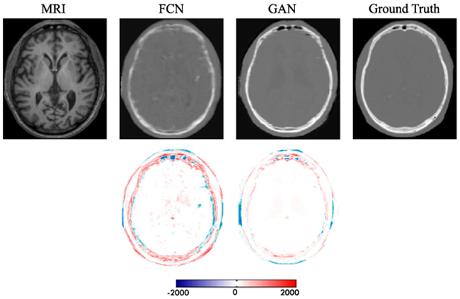
Visual comparison for impact of adversarial learning. The first row shows the synthetic CT by FCN and GAN, and the second row shows the difference map between the synthetic CT and ground truth CT. Note that FCN means the case without adversarial learning, and GAN means the proposed method with adversarial learning.

Impact of Gradient Difference Loss:

To show how the proposed gradient difference loss (GDL) works in the framework, we conduct comparisons between the case of removing GDL (No GDL, λ₃ = 0) and including GDL (With GDL, λ₃ = 1). The PSNR values are 25.2 and 25.9 for ‘No GDL’ and ‘With GDL’, respectively. Note again that these results do not include the adoption of ACM. We can visualize results in Fig. 7. It is very clear that the method ‘With GDL’ results in much sharper image. In contrast, the method ‘No GDL’ generates more blurred image. That is because GDL can enforce the gradient distribution of the generated image to be close to the gradient distribution of the real target image.

Fig. 7.

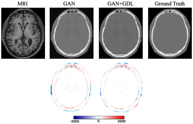
Visual comparison for impact of using the gradient difference loss (GDL). The first row shows the input MRI, two synthetic CT by two different methods, and the ground-truth CT. The second row shows difference maps between each synthetic CT and the ground-truth CT.

Auto-Context Model Refinement:

To show the contribution of ACM, we present the performance (in terms of PSNR and MAE) of the proposed method with respect to the number of iterations of ACM in Figs. 8 and 9. We can observe that both MAE and PSNR are improved gradually and consistently with iterations, especially in the first two iterations. This is because ACM could solve the short-range dependency by providing long-range context information. Considering the trade-off between the performance and the training time, we choose 2 iterations for ACM in our experiments on both datasets.

Fig. 8.

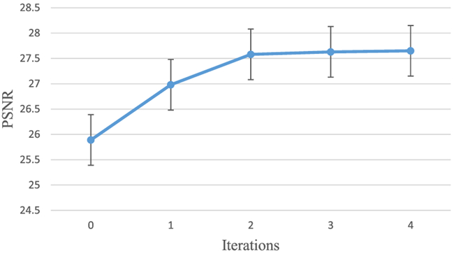
Performance (PSNR) of using ACM on the brain dataset with iterations.

Fig. 9.

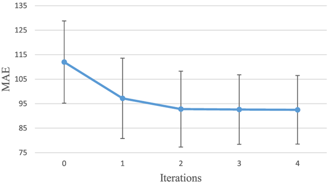
Performance (MAE) of using ACM on the brain dataset with iterations.

In order to asses the effect of the ACM on the quality of the results, we also visualize one slice from the generated brain CT of a typical dataset in the first two stages of the framework in Fig. 10. The previous effects have been summarized in Table I.

Fig. 10.

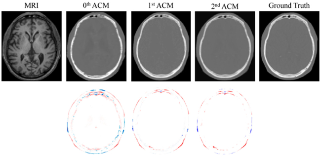
First row shows visual comparison of MR image, three synthetic CT images by applying 0th, 1st, and 2nd iterations of ACM, and the ground-truth CT image for a typical brain case. The second row shows difference maps between each iteratively estimated CT and the ground-truth CT.

TABLE I.

Results Summarizing Different Effects of Our Proposed Method on the Brain Dataset in Terms of PSNR

Method	No adv.	Adv.	Adv. + GDL	Proposed
Mean (std)	24.7(1.4)	25.2(1.4)	25.9(1.4)	27.6(1.3)

Comparison with Other Methods for the two MR-to-CT Synthesis datasets:

To qualitatively compare the estimated CT by different methods, we visualize the generated CT with the ground-truth CT in Fig. 11. We can see that the proposed algorithm can better preserve the continuity and smoothness in the results since it uses image gradient difference constraints in the image patch as discussed in Section II-A. Furthermore, we can conclude from the difference maps in Fig. 11 that the generated CT looks closer to the ground-truth CT compared to all other methods. We argue that this is due to the use of adversarial learning strategy that urges the generated images to be very similar to the real ones, so that even a complex discriminator cannot perform better than chance.

Fig. 11.

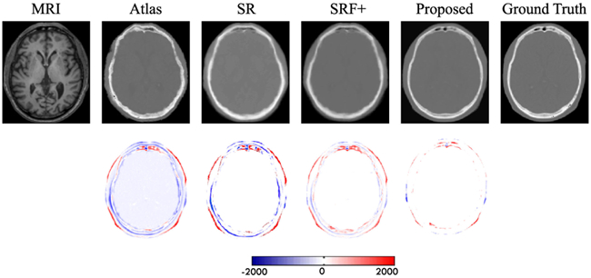
First row shows visual comparison of the MR image, the four estimated CT images by other three competing methods and our proposed method, and the ground-truth CT for a typical brain case. The second row shows difference maps between each estimated target CT and the ground-truth CT.

We also quantitatively compare the synthesis results in Table II using evaluation metrics, PSNR and MAE. Our proposed method outperforms all other competing methods in both metrics, which further demonstrates the advantage of our framework.

TABLE II.

Average MAE and PSNR on 16 Subjects from the Brain Dataset

Method	MAE		PSNR
	Mean (std)	Med.	Mean (std)	Med.
Atlas	171.5(35.7)	170.2	20.8(1.6)	20.6
SR	159.8(37.4)	161.1	21.3(1.7)	21.2
SRF + [18]	99.9(14.2)	97.6	26.3(1.4)	26.3
Proposed	92.5(13.9)	92.1	27.6(1.3)	27.6

The prediction results on the pelvic dataset by the same above methods are also shown in Fig. 12. It can be seen that our result is consistent with the ground-truth CT. The quantitative results based on the same two evaluation metrics are shown in Table III, indicating that our method outperforms other competing methods in terms of both MAE and PSNR. Specifically, our method gives an average PSNR of 34.1, which is higher than the average PSNR of 32.1 obtained by the state-of-the-art SRF+ method. The MAE values (i.e., 39.0 by our method, and 48.1 by the SRF+) further shows the improved effectiveness of our method.

Fig. 12.

First row shows visual comparison of the MR image, the estimated CT images by our method, and other competing methods, and the ground-truth CT image for the typical pelvic case. The second row shows the difference maps between estimated CT and ground- truth CT.

TABLE III.

Average MAE and PSNR on 22 Subjects from the Pelvic Dataset

Method	MAE		PSNR
	Mean (std)	Med.	Mean (std)	Med.
Atlas	66.1(6.9)	66.7	29.0(2.1)	29.6
SR	52.1(9.8)	52.3	30.3(2.6)	31.1
SRF + [18]	48.1(4.6)	48.3	32.1(0.9)	31.8
Proposed	39.0(4.6)	39.1	34.1(1.0)	34.1

We further performed Wilcoxon signed-rank test to validate whether the improvement of our proposed method compared to the previous methods is significant or not. The experimental results in Table IV show the statistical significant improvement (p < 0.05 by Wilcoxon signed-rank test).

TABLE IV.

p-Values by Performing Wilcoxon Signed-Rank Test Between Our Proposed Method and all the Previous Method for Both PSNR and MAE Values on Brain and Pelvic Datasets

Method	Brain		Pelvic
	PSNR	MAE	PSNR	MAE
Atlas	<0.01	<0.01	<0.01	<0.01
SR	<0.01	<0.01	<0.01	<0.01
SRF + [18]	<0.05	<0.05	<0.01	<0.01

B. Experiments on 3T-to-7T Synthesis

Our 3T-to-7T dataset consists of 15 subjects, each with 3T MRI (1 × 1 × 1 mm³) and 7T MRI (0.65 × 0.65 × 0.65 mm³), scanned using 3T and 7T MRI scanners respectively. The 7T MRI provides higher resolution and contrast than the 3T MRI, thus benefiting early diagnosis of brain diseases. These images are all linearly aligned and skull-stripped to remove non-brain regions.

Impact of Adversarial Learning:

To show the contribution of the adversarial learning, we conduct comparison experiments between the traditional FCN (i.e., just the generator shown in Fig. 2) and the proposed GAN model. The PSNR values are 26.15(1.27) and 26.88(1.25) by the traditional FCN and the one with adversarial learning, respectively. Note that these results do not include the GDL, residual learning and ACM. We can visualize results in Fig. 13, where the leftmost image is the 3T MRI, and the rightmost image is the ground-truth 7T MRI. We can clearly see that the generated data using the GAN approach has less artifacts than the traditional FCN, by estimating an image that is closer to the desired output quantitatively and qualitatively.

Fig. 13.

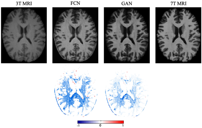
Visual comparison to demonstrate the impact of using the adversarial learning for the 3T-to-7T dataset. The first row shows 3T MRI, two synthetic 7T MRI by two methods, and ground-truth 7T MRI. The second row shows difference maps between each synthetic 7T MRI and ground-truth 7T MRI. Note that FCN means the case without adversarial learning, and GAN means the case with adversarial learning.

Impact of Gradient Difference Loss:

To show how the proposed gradient difference loss (GDL) work in the framework, we conduct the same comparison experiments as the previous datasets. The PSNR values are 26.83(1.25) and 27.18(1.24) for the method ‘No GDL’ and the method ‘With GDL’, respectively. These results do not include the residual learning and ACM. We can visualize results in Fig. 14. Similar conclusions to those discussed above for the previous datasets can be made, i.e., obtaining much sharper and more realistic images.

Fig. 14.

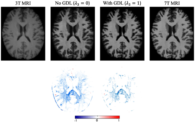
Visual comparison to demonstrate the impact of using the gradient difference loss. The image obtained via GDL is more realistic and sharper. The first row shows 3T MRI, the synthetic 7T MRI by two methods, and ground-truth 7T MRI; the second row shows difference maps between each synthetic 7T MRI and the ground-truth 7T MRI.

Impact of Residual Learning:

To show how the proposed long-term residual learning unit work in the framework, we conduct comparison experiments (i.e., using a GAN without this residual unit and a GAN with this unit, denoted as ‘GAN’ and ‘ResGAN’ respectively) to validate it in this dataset. The PSNR values are 27.18(1.24) and 27.69(1.22) by the method ‘GAN’ and the method ‘ResGAN’, respectively. Note that these results do not include the ACM. We have visualized the generated 7T MRI in Fig. 15. The ‘ResGAN’ generates a clearer 7T MRI compared to ‘GAN’, especially for the details. This is mainly due to better convergence after using residual learning concept, which has been validated in Fig. 16.

Fig. 15.

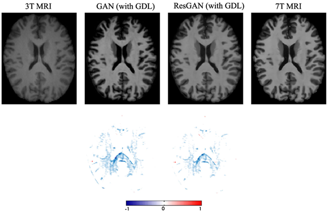
Visual comparison to demonstrate the impact of using the residual learning. The first row shows synthetic 7T MRI, and the second row shows the difference maps between the synthetic 7T MRI and ground truth 7T MRI.

Fig. 16.

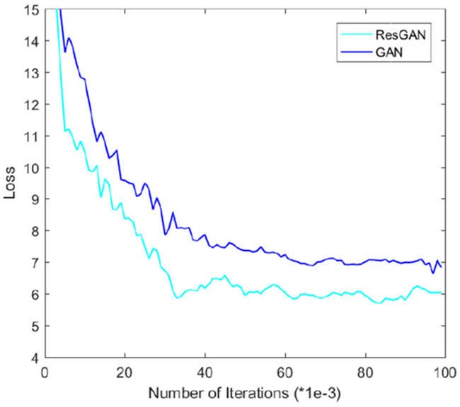
Mean squared loss (MSE) of the generator in GAN and Res-GAN on the testing dataset with respect to different training iterations.

More Evaluation for the Image Reconstruction Quality:

Since the contrast is quite high with subcortical regions (such as thalamus and putamen) in 7T images compared to 3T, we also show a slice of the generated image in Fig. 17 in order to verify if this contrast is produced. The previous investigated effects have been summarized in Table V.

Fig. 17.

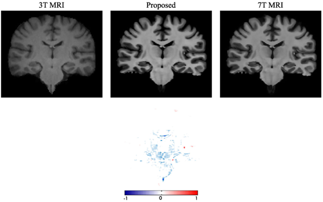
Visualization for subcortical regions with 3T MRI, the synthetic 7T MRI, and the ground-truth 7T MRI. Thesecond row shows a difference map between the ground-truth 7T MRI and the synthetic 7T MRI.

TABLE V.

Results Summarizing Different Effects of Our Proposed Method on the 3T-to-7T Dataset in Terms of of PSNR

Method	No Adv.	Adv.	Adv. + GDL	ResGAN	ResGAN + ACM
Mean(std)	26.15(1.27)	26.83(1.25)	27.18(1.24)	27.69(1.22)	27.93(1.18)

On the other hand, it is important to notice that we have been evaluating the quality of the generated images with a global metric such as the PSNR. In a medical setting however, it is important to asses if the image is anatomically correct. Trying to evaluate the medical applicability, we decided to try a segmentation algorithm on both the generated image and the real 7T. In particular, we train an FCN (U-NET [52]) in order to segment 7T images into White Matter (WM), Gray Matter (GM), and Cerebrospinal Fluid (CSF). We then evaluate the Dice Index of the segmentation maps obtained using the original 7T and the generated 7T as inputs to the network. We show a slice of the segmentation maps obtained in Fig. 18, and show the Dice Index in Table VI. The results show that the synthetic 7T MRI produces a segmentation map that is very close to that one produced by the real 7T in terms of Dice Index, and both of them largely outperform the results obtained by directly segmenting the 3T MRI. These results imply that the synthetic images have high quality and could be applicable to image segmentation.

Fig. 18.

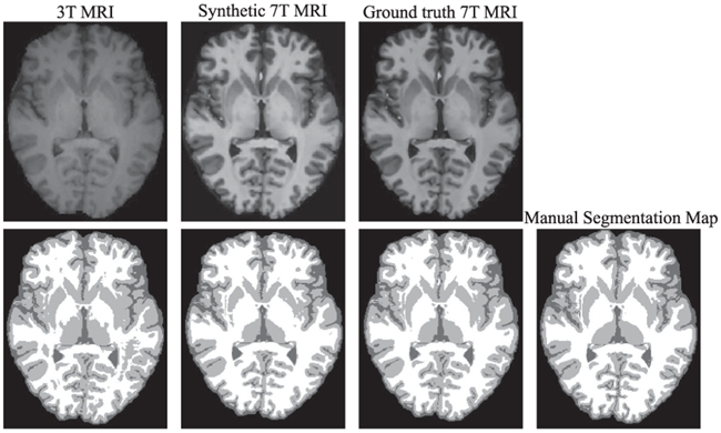
Visual comparison of segmentation results for a typical subject by using different input data (3T MRI, synthetic 7T MRI, and ground-truth 7T MRI). The first row is the MRI, and the second shows the segmented slices as well as the manual segmentation map.

TABLE VI.

Performance of Segmentation on the MRI Dataset in Terms of Dice Index and its Corresponding Standard deviation

Input	WM	GM	CSF
3T MRI	80.35(2.02)	85.49(1.08)	88.75(0.93)
Synthetic 7T MRI	86.84(1.84)	91.68(0.92)	95.96(0.88)
Ground-truth 7T MRI	87.70(1.76)	92.33(0.86)	96.58(0.90)

Comparison with Other Methods:

We compare our methods with several state-of-the-art methods: 1) HM: Histogram Matching, which matches the intensity distribution of an image with the intensity distribution of a target image; 2) LIS: Local Image Similarity [53], which synthesizes the target image using multiple atlases propagated according to local image similarity measures; 3) M-CCA: Multi-level CCA [54], which conducts a hierarchical reconstruction based on group sparsity in a novel multi-level CCA framework; 4) CNN: a 3D Convolutional Neural Networks [4], which learns non-linear mapping between the source image and target image. We list the experimental results in Table VII. The proposed framework outperforms the baselines methods by a big margin, which further validates the effectiveness of our proposed generative adversarial networks.

TABLE VII.

Comparison of the Performances of Different Methods on the 3T-to-7T Dataset in Terms of PSNR

Method	HM	LIS	M-CCA	CNN	Proposed
Mean	21.10	24.33	25.41	26.50	27.93
(std)	(1.44)*	(1.26)*	(1.20)*	(1.22)*	(1.18)

The p-values by performing Wilcoxon signed-rank test between our proposed method and all other methods are also reported, and we use “*” to denote p < 0.01.

IV. Conclusion

We have proposed a supervised deep convolutional model for estimating a target image from a source image via adversarial learning, even for the cases where the target and the source images belong to different modalities. Moreover, a special loss function (i.e., image gradient difference loss) is proposed to alleviate the blurry issue of the generated target image. We have also extended the residual learning unit to long-term residual connection so that the network can be trained more easily. Finally, the performance is iteratively improved by the use of ACM since the context of the GAN is effectively enlarged during the training process, which makes it context-aware. We have validated our proposed model on two tasks: 1) predicting CT data from corresponding MRI data and 2) converting 3T MRI to 7T MRI. The experiments demonstrate that our proposed method can significantly outperform the three state-of-the-art methods in all the tasks and all datasets. The experiments also indicate that our proposed model can be generalized to various medical image synthesis tasks with promising results.

References

- [1].Kinahan PE et al. , “Attenuation correction for a combined 3d pet/ct scanner,” Med. Phys, vol. 25, no. 10, pp. 2046–2053, 1998. [DOI] [PubMed] [Google Scholar]
- [2].Beisteiner R et al. , “Clinical fmri: Evidence for a 7t benefit over 3t,” Neuroimage, vol. 57, no. 3, pp. 1015–1021, 2011. [DOI] [PMC free article] [PubMed] [Google Scholar]
- [3].Bahrami K et al. , “Hierarchical reconstruction of 7t-like images from 3t mri using multi-level cca and group sparsity,” in Proc. Int. Conf. Med. Image Comput. Comput.-Assisted Intervention, Springer, 2015, pp. 659–666. [DOI] [PMC free article] [PubMed] [Google Scholar]
- [4].Bahrami K et al. , “Convolutional neural network for reconstruction of 7t-like images from 3t mri using appearance and anatomical features,” in Proc. Int. Workshop Large-Scale Annotation Biomed. Data Expert Label Synthesis, Springer, 2016, pp. 39–47. [Google Scholar]
- [5].Farsiu S et al. , “Advances and challenges in super-resolution,” Int. J. Imaging Syst. Technol, vol. 14, no. 2, pp. 47–57, 2004. [Google Scholar]
- [6].Greenspan H, “Super-resolution in medical imaging,” Comput. J, vol. 52, no. 1, pp. 43–63, 2009. [Google Scholar]
- [7].Hefnawy AA, Super Resolution Challenges and Rewards. Paris, France: Atlantis Press, 2010, pp. 163–206, doi: 10.2991/978-94-91216-30-5_6. [DOI] [Google Scholar]
- [8].Berker Y et al. , “Mri-based attenuation correction for hybrid pet/mri systems: A 4-class tissue segmentation technique using a combined ultrashort-echo-time/dixon mri sequence,” J. Nucl. Med, vol. 53, no. 5, pp. 796–804, 2012. [DOI] [PubMed] [Google Scholar]
- [9].Zaidi H et al. , “Magnetic resonance imaging-guided attenuation and scatter corrections in three-dimensional brain positron emission tomography,” Med. Phys, vol. 30, no. 5, pp. 937–948, 2003. [DOI] [PubMed] [Google Scholar]
- [10].Catana C et al. , “Toward implementing an mri-based pet attenuation-correction method for neurologic studies on the mr-pet brain prototype,” J. Nucl. Med, vol. 51, no. 9, pp. 1431–1438, 2010. [DOI] [PMC free article] [PubMed] [Google Scholar]
- [11].Hofmann M et al. , “Mri-based attenuation correction for pet/mri: A novel approach combining pattern recognition and atlas registration,” J. Nucl. Med, vol. 49, no. 11, pp. 1875–1883, 2008. [DOI] [PubMed] [Google Scholar]
- [12].Zhang Y et al. , “Optimizing spatial patterns with sparse filter bands for motor-imagery based brain-computer interface,” J. Neurosci. Methods, vol. 255, pp. 85–91, 2015. [DOI] [PubMed] [Google Scholar]
- [13].Ye DH et al. , Modality Propagation: Coherent Synthesis of Subject-Specific Scans with Data-Driven Regularization. Berlin, Germany: Springer-Verlag, 2013, pp. 606–613, doi: 10.1007/978-3-642-40811-3_76. [DOI] [PubMed] [Google Scholar]
- [14].Burgos N et al. , “Attenuation correction synthesis for hybrid pet-mr scanners: Application to brain studies,” IEEE Trans. Med. Imaging, vol. 33, no. 12, pp. 2332–2341, Dec. 2014. [DOI] [PubMed] [Google Scholar]
- [15].Manjón JV et al. , “Mri superresolution using self-similarity and image priors,” J. Biomed. Imaging, vol. 2010, p. 17, 2010. [DOI] [PMC free article] [PubMed] [Google Scholar]
- [16].Jog A et al. , “Improving magnetic resonance resolution with supervised learning,” in Proc. IEEE 11th Int. Symp. Biomed. Imaging, 2014, pp. 987–990. [DOI] [PMC free article] [PubMed] [Google Scholar]
- [17].Coupé P et al. , “Collaborative patch-based super-resolution for diffusion-weighted images,” NeuroImage, vol. 83, pp. 245–261, 2013. [DOI] [PubMed] [Google Scholar]
- [18].Huynh T et al. , “Estimating ct image from mri data using structured random forest and auto-context model,” IEEE Trans. Med. Imaging, vol. 35, no. 1, pp. 174–183, Jan. 2016. [DOI] [PMC free article] [PubMed] [Google Scholar]
- [19].Alexander DC et al. , “Image quality transfer via random forest regression: Applications in diffusion mri,” in Proc. Int. Conf. Med. Image Comput. Comput.-Assisted Intervention, Springer, 2014, pp. 225–232. [DOI] [PubMed] [Google Scholar]
- [20].Zhang Y et al. , “Sparse bayesian classification of eeg for brain-computer interface,” IEEE Trans. Neural Netw. Learning Syst, vol. 27, no. 11, pp. 2256–2267, Nov. 2016. [DOI] [PubMed] [Google Scholar]
- [21].Wu Y et al. , “Prediction of ct substitutes from mr images based on local sparse correspondence combination,” in Proc. Int. Conf. Med. Image Comput. Comput.-Assisted Intervention, Springer, 2015, pp. 93–100. [Google Scholar]
- [22].Zhan Y and Shen D, “Automated segmentation of 3d us prostate images using statistical texture-based matching method,” in Proc. Int. Conf. Med. Image Comput. Comput.-Assisted Intervention, Springer, 2003, pp. 688–696. [Google Scholar]
- [23].Feng Q et al. , “Segmenting ct prostate images using population and patient-specific statistics for radiotherapy,” Med. Phys, vol. 37, no. 8, pp. 4121–4132, 2010. [DOI] [PMC free article] [PubMed] [Google Scholar]
- [24].Shen D et al. , “Optimized prostate biopsy via a statistical atlas of cancer spatial distribution,” Med. Image Anal, vol. 8, no. 2, pp. 139–150, 2004. [DOI] [PubMed] [Google Scholar]
- [25].Vemulapalli R et al. , “Unsupervised cross-modal synthesis of subject-specific scans,” in Proc. IEEE Int. Conf. Comput. Vis, Dec. 2015, pp. 630–638. [Google Scholar]
- [26].Krizhevsky A et al. , “Imagenet classification with deep convolutional neural networks,” in Proc. Adv. Neural Inform. Process. Syst, 2012, pp. 1097–1105. [Google Scholar]
- [27].LeCun Y et al. , “Deep learning,” Nature, vol. 521, no. 7553, pp. 436–444, 2015. [DOI] [PubMed] [Google Scholar]
- [28].He K et al. , “Deep residual learning for image recognition,” in Proc. IEEE Conf. Comput. Vis. Pattern Recog., 2016, pp. 770–778. [Google Scholar]
- [29].Liao S, Gao Y, Oto A, and Shen D, “Representation learning: A unified deep learning framework for automatic prostate mr segmentation,” in Proc. Int. Conf. Med. Image Comput. Comput.-Assisted Intervention, Springer, 2013, pp. 254–261. [DOI] [PMC free article] [PubMed] [Google Scholar]
- [30].Dong C et al. , “Learning a deep convolutional network for image super-resolution,”in Proc. Eur. Conf. Comput. Vis, Springer, 2014, pp. 184–199. [Google Scholar]
- [31].Kim J et al. , “Deeply-recursive convolutional network for image super-resolution,” in Proc. IEEE Conf. Comput. Vis. Pattern Recog., 2016, pp. 1637–1645. [Google Scholar]
- [32].Li R et al. , “Deep learning based imaging data completion for improved brain disease diagnosis,” in Proc. Int. Conf. Med. Image Comput. Comput.-Assisted Intervention, Springer, 2014, pp. 305–312. [DOI] [PMC free article] [PubMed] [Google Scholar]
- [33].Huang Y, Shao L and Frangi A, “Simultaneous super-resolution and cross-modality synthesis of 3d medical images using weakly-supervised joint convolutional sparse coding,” IEEE Conf. Comput. Vision and Pattern Recognition (CVPR), Honolulu, USA, 2017. [Google Scholar]
- [34].Dong C et al. , “Image super-resolution using deep convolutional networks,” IEEE Trans. Pattern Anal. Mach. Intell, vol. 38, no. 2, pp. 295–307, Feb. 2016. [DOI] [PubMed] [Google Scholar]
- [35].Mathieu M, Couprie C, LeCun Y, “Deep multi-scale video prediction beyond mean square error,” Int. Conf. Learning Representations (ICLR), Puerto Rico, 2016. [Google Scholar]
- [36].Ledig C et al. , “Photo-realistic single image super-resolution using a generative adversarial network,” IEEE Conf. Computer Vision and Pattern Recognition (CVPR), Honolulu, USA, 2017. [Google Scholar]
- [37].Nie D et al. , “Medical image synthesis with context-aware generative adversarial networks,” in Proc. Int. Conf. Med. Image Comput. Comput.-Assisted Intervention, 2017, pp. 417–425. [DOI] [PMC free article] [PubMed] [Google Scholar]
- [38].Goodfellow I et al. , “Generative adversarial nets,” in Proc. Adv. Neural Inform. Process. Syst, 2014, pp. 2672–2680. [Google Scholar]
- [39].Long J et al. , “Fully convolutional networks for semantic segmentation,” in Proc. IEEE Conf. Comput. Vis. Pattern Recog., 2015, pp. 3431–3440. [Google Scholar]
- [40].Nie D et al. , “Fully convolutional networks for multi-modality isointense infant brain image segmentation,” in Proc. IEEE 13th Int. Symp. Biomed. Imaging, 2016, pp. 1342–1345. [DOI] [PMC free article] [PubMed] [Google Scholar]
- [41].Nie D et al. , “3-D fully convolutional networks for multimodal isointense infant brain image segmentation,” IEEE Trans. Cybern, to be published, doi: 10.1109/TCYB.2018.2797905. [DOI] [PMC free article] [PubMed] [Google Scholar]
- [42].Han X, “Mr-based synthetic ct generation using a deep convolutional neural network method,” Med. Phys, vol. 44, no. 4, pp. 1408–1419, 2017. [DOI] [PubMed] [Google Scholar]
- [43].Nie D et al. , “Estimating ct image from mri data using 3D fully convolutional networks,” in Proc. Int. Workshop Large-Scale Annotation Biomed. Data Expert Label Synthesis, Springer, 2016, pp. 170–178. [DOI] [PMC free article] [PubMed] [Google Scholar]
- [44].Radford A et al. , “Unsupervised representation learning with deep convolutional generative adversarial networks,” unpublished paper, 2015. [Online]. Avaiable: https://arxiv.org/abs/1511.06434v1 [Google Scholar]
- [45].Luo W et al. , “Understanding the effective receptive field in deep convolutional neural networks,” in Proc. Adv. Neural Inform. Process. Syst, 2016, pp. 4898–4906. [Google Scholar]
- [46].Yu F and Koltun V, “Multi-scale context aggregation by dilated convolutions,” Int. Conf. Learning Representations (ICLR), Puerto Rico, 2016. [Google Scholar]
- [47].Kim J et al. , “Accurate image super-resolution using very deep convolutional networks,” in Proc. IEEE Conf. Comput. Vis. Pattern Recog., 2016, pp. 1646–1654. [Google Scholar]
- [48].Tu Z and Bai X, “Auto-context and its application to high-level vision tasks and 3d brain image segmentation,” IEEE TPAMI, vol. 32, no. 10, pp. 1744–1757, Oct. 2010. [DOI] [PubMed] [Google Scholar]
- [49].Heinrich MP et al. , “Mind: Modality independent neighbourhood descriptor for multi-modal deformable registration,” Med. Image Anal, vol. 16, no. 7, pp. 1423–1435, 2012. [DOI] [PubMed] [Google Scholar]
- [50].Avants BB et al. , “Symmetric diffeomorphic image registration with cross-correlation: Evaluating automated labeling of elderly and neurodegenerative brain,” Medi. Image Anal, vol. 12, no. 1, pp. 26–41, 2008. [DOI] [PMC free article] [PubMed] [Google Scholar]
- [51].Vercauteren T et al. , “Diffeomorphic demons: Efficient non-parametric image registration,” NeuroImage, vol. 45, no. 1, pp. S61–S72, 2009. [DOI] [PubMed] [Google Scholar]
- [52].Ronneberger O et al. , “U-net: Convolutional networks for biomedical image segmentation,” in Proc. Int. Conf. Med. Image Comput. Comput.-Assisted Intervention, Springer, 2015, pp. 234–241. [Google Scholar]
- [53].Burgos N et al. , “Attenuation correction synthesis for hybrid pet-mr scanners: Application to brain studies,” IEEE Trans. Med. Imaging, vol. 33, no. 12, pp. 2332–2341, Dec. 2014. [DOI] [PubMed] [Google Scholar]
- [54].Bahrami K et al. , “Reconstruction of 7t-like images from 3t mri,” IEEE Trans. Med. Imaging, vol. 35, no. 9, pp. 2085–2097, Sep. 2016. [DOI] [PMC free article] [PubMed] [Google Scholar]