A Hierarchical Geodesic Model for Diffeomorphic Longitudinal Shape Analysis

Abstract

Hierarchical linear models (HLMs) are a standard approach for analyzing data where individuals are measured repeatedly over time. However, such models are only applicable to longitudinal studies of Euclidean data. In this paper, we propose a novel hierarchical geodesic model (HGM), which generalizes HLMs to the manifold setting. Our proposed model explains the longitudinal trends in shapes represented as elements of the group of diffeomorphisms. The individual level geodesics represent the trajectory of shape changes within individuals. The group level geodesic represents the average trajectory of shape changes for the population. We derive the solution of HGMs on diffeomorphisms to estimate individual level geodesics, the group geodesic, and the residual geodesics. We demonstrate the effectiveness of HGMs for longitudinal analysis of synthetically generated shapes and 3D MRI brain scans.

1. Introduction

A longitudinal study of neuroanatomical aging, development and disease progression necessitates modeling anatomical changes over time. A convenient representation of anatomical variability is via maps of diffeomorphisms, which are topology-preserving smooth and invertible transformations of a template image. Recently proposed methods, such as geodesic regression [5,10,11], effectively represent smooth trajectories of changes in anatomy. However, regression is not an appropriate model of longitudinal data.

Related work [3, 4, 7] estimate the group trajectory by averaging individual trajectories in the diffeomorphic setting. Durrleman et. al [3] estimates a spatiotemporal piecewise geodesic atlas. Although this method estimates a continuous evolution of spatial change, it does not guarantee smoothness of the resulting average estimate across the time span. The average shape trajectory estimates by Fishbaugh et. al [4] are also not guaranteed to be smooth in time. The approach based on stationary velocity fields presented in [7] does not model distances between trajectories, which makes it difficult to compare the differences in trends for statistical analysis.

Another important shortcoming of the contemporary methods of averaging trajectories is that they do not apply when the time ranges of measurements of individuals are staggered. For instance, [3] and [4] both require extrapolation and resampling for each individual trajectory estimates outside their time-range before an average evolution of the population can be computed. Muralidharan et. al [9] address these problems and estimate smooth geodesic representations for individual and group trends for a population of staggered individual measurements. They utilize a Sasaki metric on the tangent bundle of the manifold of finite-dimensional shapes to compare geodesic trends. However, their methods are difficult to apply to the infinite-dimensional space of diffeomorphic transformations, due to the need for curvature computations of the underlying manifold.

In this paper, we present a hierarchical geodesic model (HGM) on diffeomorphisms that generalizes classical hierarchical linear models (HLMs) on Euclidean spaces. HGMs utilize the metric on the space of diffeomorphisms to define the group geodesic given a population of geodesics. It applies to commonly occurring unbalanced designs in medical imaging data where measurements are staggered, i.e., not every individual is measured at the same time points. The consequence of this modeling is an estimate of a smooth “average geodesic” and a common reference coordinate system to represent longitudinal trends of multiple individuals for longitudinal studies.

2. Hierarchical Geodesic Models

We begin by defining HGMs in the simplest scenario in which the data lie in a Euclidean space. In this case, the geodesic models of longitudinal trends reduce to straight lines, and we give a procedure for estimation of model parameters defining the group level trend in a hierarchical fashion. We later present the generalization of this model and its estimation to diffeomorphisms.

2.1. Hierarchical Geodesic Models in Euclidean Space

Consider the univariate longitudinal case with independent time variable, t, and dependent response variable, y. Say we are given a population of N individuals with M_i measurements for the ith individual. The design can be unbalanced, meaning there are potentially a different number of measurements for each individual. Denote y_ij as the jth measurement of the ith individual at time t_ij. Motivated by classical hierarchical linear models [6] for repeated measurements, this is modeled in two levels as

Group Level:	Individual Level:
$a_i~\mathcal{N}(\alpha +\beta t_{i0},{\sigma }_I^2)$	$y_{ij}~\mathcal{N}(a_i+b_i(t_{ij}-t_{i0}),{\sigma }_i^2)$
$b_i~\mathcal{N}(\beta ,{\sigma }_S^2)$

The estimation of the parameters for this model proceeds in two stages. First, the individual level parameters a_i and b_i are estimated. These estimates are then used to estimate α and β at the group level. The solution to this model thus corresponds to minimizing the negative log-likelihood at individual and group levels, respectively, where

$$-\log (p(y_{\mathit{ij}}\mid a_i,b_i))=\frac{1}{2{\sigma }_i^2}\sum _{j=1}^{M_i}{[y_{\mathit{ij}}-(a_i+b_i(t_{\mathit{ij}}-t_{i0}))]}^2$$ (1)

$$-\log (p(a_i,b_i\mid \alpha ,\beta ))=\frac{1}{2{\sigma }_I^2}\sum _{i=1}^N{[(\alpha +\beta t_{i0})-a_i]}^2+\frac{1}{2{\sigma }_S^2}\sum _{i=1}^N{[\beta -b_i]}^2$$ (2)

Individual level:

The solution for the slope-intercept pair, a_i,b_i, in the individual level that minimize (1) is given by the standard ordinary least-squares regression solution. An equivalent solution more directly generalizable to the diffeomorphic case is to solve this problem as an optimal control, as detailed in [10]. This is done by adding Lagrange multipliers to constrain the curves to be straight lines and derive the system of equation termed the adjoint equations.

Group level:

The maximum likelihood group estimate represents an “average line”, α(t), that best matches the individual lines, (a_i, b_i), in least-squares sense. From an optimal control viewpoint, we add Lagrange multipliers to constrain the curve α(t) to be a straight line. This is done by introducing time-dependent adjoint variables, λ^α and λ^β, in the log-likelihood in (2), giving

$$\mathcal{E}(\alpha ,\beta )={\int }_0^{t_N}({\lambda }^{\alpha }(\stackrel{.}{\alpha }-\beta )+{\lambda }^{\beta }\stackrel{.}{\beta })\mathit{dt}+\frac{1}{2}\sum _{i=1}^N(\frac{1}{{\sigma }_I^2}{(\alpha (t_i)-a_i)}^2+\frac{1}{{\sigma }_S^2}{(\beta (t_i)-b_i)}^2)$$

The gradients of this functional are ${\delta }_{\alpha (0)}\mathcal{E}=-{\lambda }^{\alpha }(0^{-})$ and ${\delta }_{\beta (0)}\mathcal{E}=-{\lambda }^{\beta }(0^{-})$. These are evaluated by integrating backwards the adjoint equations, $-{\stackrel{.}{\lambda }}^{\alpha }=0$, and ${\stackrel{.}{\lambda }}^{\beta }=-{\lambda }^{\alpha }$, subject to the following boundary and jump conditions:

$$\begin{array}{cc}\hfill {\lambda }^{\alpha }(t_N)=-\frac{1}{{\sigma }_I^2}(\alpha (t_N)-a_N)& \hfill {\lambda }^{\beta }(t_N)=-\frac{1}{{\sigma }_S^2}(\beta (t_N)-b_N)\\ \hfill {\lambda }^{\beta }(t_k^{+})-{\lambda }^{\beta }(t_k^{-})=\frac{1}{{\sigma }_S^2}(\beta (t_i)-b_i)& \hfill {\lambda }^{\alpha }(t_k^{+})-{\lambda }^{\alpha }(t_k^{-})=\frac{1}{{\sigma }_I^2}(\alpha (t_i)-a_i)\end{array}$$

Notice that unlike least squares regression, the velocity term in the group log-likelihood at group level also influences the group estimate. In particular, the jumps in integrating λ^β are interpreted as the forces by the initial velocities pulling the group geodesic. The solution for α(0) and β(0) in this Euclidean case corresponds to the solution of the linear system Ax = b, where:

$$A=\left(\begin{array}{cc}\hfill N\frac{1}{{\sigma }_I^2}\hfill & \hfill \frac{1}{{\sigma }_I^2}\sum _{i=0}^N{t}_i\hfill \\ \hfill \frac{1}{{\sigma }_I^2}\sum _{i=0}^N{t}_i\hfill & \hfill N\frac{1}{{\sigma }_S^2}+\frac{1}{{\sigma }_I^2}\sum _{i=0}^N{t}_i^2\hfill \end{array}\right),b=\left(\begin{array}{c}\hfill \frac{1}{{\sigma }_I^2}\sum _{i=0}^N{a}_i\hfill \\ \hfill \frac{1}{{\sigma }_I^2}\sum _{i=0}^N{a}_i{t}_i+\frac{1}{{\sigma }_S^2}\sum _{i=0}^N{b}_i\hfill \end{array}\right)$$

Notice that if there is no slope term in the energy functional, i.e., as ${\sigma }_S^2\to \infty$, this reduces to the standard ordinary least squares solution for linear regression. An example of synthetically generated longitudinal data is shown in Figure 1. This example illustrates the importance of modeling correlations within each individual by including individual slope terms in the likelihood function. Ignoring these correlations leaves us with a simple linear regression fit to the data, which does not reflect the longitudinal trends that individuals experience. In contrast, the group trend, α(t), estimated in the hierarchical model by including slope terms, better summarizes the average behavior of the individual trends.

Fig. 1.

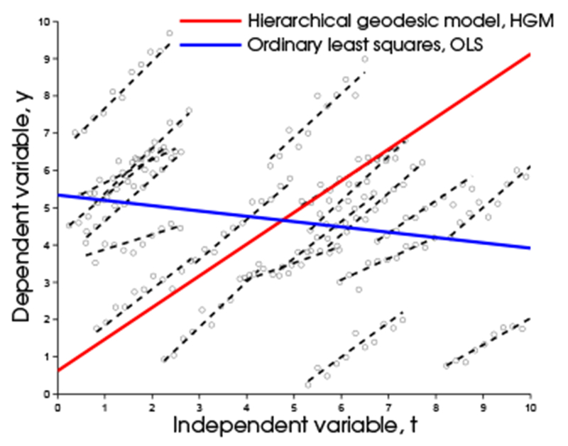
Comparing HGM and OLS in Euclidean space.

2.2. Background on Diffeomorphisms

We follow the well-established framework of large deformation diffeomorphic metric mapping (LDDMM) [2, 12]. Before introducing our longitudinal model on manifold of anatomical shape changes, we briefly review some necessary background of the mathematical framework of diffeomorphisms.

Diffeomorphisms:

Let Ω be the coordinate space of the image, I. A diffeomorphism, ϕ(t), is constructed by the integration of an ordinary differential equations (ODE) on Ω defined via a smooth, time-indexed velocity field, v(t). The deformation of an image I by ϕ is defined as the action of the diffeomorphism, given by ϕ ∘ I = I ∘ ϕ⁻¹. The choice of a self-adjoint differential operator, L determines the right-invariant Riemannian structure on the collection of velocity fields with the norm defined as, ${\parallel v\parallel }^2={\int }_{\Omega }(Lv(x),v(x))\mathit{dx}$.

Deformation momenta and EPDiff evolution:

The tangent space at identity, V = T_IdDiff(Ω) consists of all vector fields with finite norm. Its dual space, $V^{\ast }=T_{\mathrm{Id}}^{\ast }\mathrm{Diff}(\Omega )$ consists of vector-valued distributions over Ω. The velocity, v ∈ V, maps to its dual deformation momenta, m ∈ V*, via the operator L such that m = Lv and v = Km. The operator K : V* → V denotes the inverse of L. Note that constraining ϕ to be a geodesic with initial momentum, m(0) implies that ϕ, m, and I all evolve in a way entirely determined by the metric L, and that the deformation is determined entirely by the initial deformation momenta, m(0). Given the initial velocity, v(0) ∈ V, or equivalently, the initial momentum, m(0) ∈ V*, the geodesic path ϕ(t) is constructed as per the following EPDiff equations [1, 8]:

$${\partial }_{t}m=-{\mathrm{ad}}_v^{\ast }m=-{(\mathit{Dv})}^{T}m-\mathit{Dmv}-(\text{div}v)m$$ (3)

where D denotes the Jacobian matrix, and the operator ad* is the dual of the negative Jacobi-Lie bracket of vector fields [1, 8, 12] such that, ad_vw = −[v, w] = Dvw — Dwv. The deformed image I(t) = I(0)∙ϕ⁻¹(t), evolves via: ∂_tI = −v∙∇I.

2.3. Hierarchical Geodesic Models for Diffeomorphisms

Similar to the setup discussed for Euclidean data, we are given a population of N individuals with M_i measurements for the ith individual. There can be a variable number of measurements for each individual. Denote H_ij as the jth measured image of the ith individual at time t_ij.

Figure 2 shows a schematic of the HGM. We model geodesic trend for an individual with a diffeomorphism, ξ_i(t) (brown). The initial image, or intercept, J_i(0), and the initial momenta, or slope, n_i(0), fully parameterize the trajectory for the ith individual. At the group level, we model the group geodesic trend with the diffeomorphism, ψ(t), (red) starting at identity, parameterized by initial momenta, m(0). Let ϕ_i denote the diffeomorphism that matches individual baseline J_i(0) from identity and ρ_i denote the residual geodesic between ψ(t_i) and ϕ_i: ρ_i = ϕ_i ∘ ψ⁻¹(t_i). The initial momenta, p_i(0), parameterize residual, ρ_i.

Fig. 2.

Hierarchical geodesic modeling in diffeomorphisms.

We now present the hierarchical geodesic estimation procedure on diffeomorphisms in two stages. For the first stage, we note that estimates at individual level amounts to solving N geodesic regression problems for each individual as proposed in [10, 11]. We briefly review it here under the vectorized deformation momenta formulation (details in [11]). In the second stage at the group level, we address the more interesting question of averaging the individual geodesics in the space of diffeomorphisms.

Individual level:

Given M_i observed images H_ij at time points t_ij for an individual such that j = 1,…, M_i, the geodesic that passes closest, in the least squares sense, to the data minimizes the energy functional:

$$\mathcal{E}(J_i(0),n_i(0))=\frac{1}{2}{\parallel n_i(0)\parallel }_K^2+\frac{1}{2{\sigma }_i^2}\sum _{j=1}^{M_i}{\parallel J_i(t_{\mathit{ij}})-H_{\mathit{ij}}\parallel }_{L^2}^2$$

where J_i(0) and m_i(0) are the initial “intercept” and “slope” to be estimated that completely parameterize the geodesic for the i^th individual. Here, Ji(t) = ξ_i(t) ∙ J_i(0) and ||.||_K is the norm defined by the kernel, K, in the dual space of momenta, as per the metric induced by Sobolev operator, L, on velocity fields. This is done by adding time-dependent Lagrange multipliers, ${\widehat{n}}_i$, ${\widehat{J}}_i$, and ${\widehat{w}}_i$, to constrain ξ_i(t) to be along the EPDiff geodesic path:

$$\tilde{\mathcal{E}}(J_i(0),n_i(0))=\mathcal{E}+{\int }_0^1{\langle {\widehat{n}}_i,{\stackrel{.}{n}}_i+{\mathrm{ad}}_{w_i}^{\ast }{n}_i\rangle }_{L^2}\mathit{dt}+{\int }_0^1{\langle {\widehat{J}}_i,{\stackrel{.}{J}}_i+\nabla J_i\cdot w_i\rangle }_{L^2}\mathit{dt}+{\int }_0^1{\langle {\widehat{w}}_i,n_i-L{w}_i\rangle }_{L^2}\mathit{dt}.$$

The variation of $\tilde{\mathcal{E}}$ with respect to the initial momenta is

$${\delta }_{n_i(0)}\tilde{\mathcal{E}}=K\star n_i(0)-{\widehat{n}}_i(0)$$ (4)

The optimality conditions for n_i and J_i result in the time-dependent adjoint system of ODEs which are integrated backward in time to obtain ${\widehat{n}}_i(0)$ to compute gradient update in (4). The variation of $\tilde{\mathcal{E}}$ with respect to the initial image, ${\delta }_{J_i(0)}\tilde{\mathcal{E}}$, can be directly computed from the energy functional, $\tilde{\mathcal{E}}$. Since $J_i(t)={\xi }_i(t)\cdot J_i(0)=J_i(0)\circ {\xi }_i^{-1}(t)$, a change of variables for ξ_i, followed by taking the derivative with respect to J_i(0), results in the closed form solution for optimum initial image, J_i(0), as

$$J_i(0)=\frac{\sum _{j=1}^{M_i}{H}_{\mathit{ij}}\circ {\xi }_i(t_{\mathit{ij}})\mid D{\xi }_i(t_{\mathit{ij}})\mid }{\sum _{j=1}^{M_i}\mid D{\xi }_i(t_{\mathit{ij}})\mid }.$$

Note that the solution to the geodesic regression problem presented in [10] is based on optimization over scalar deformation momentum. In our formulation, the evolution of the geodesic and adjoint system is decoupled from the template image resulting in a closed-form for image update. In the discussion that follows, for clarity and ease of notation, we will use J_i = J_i (0) to denote the initial “intercept” and n_i = n_i(0) to denote initial “slope” for an individual.

Group level:

At the group level (Figure 2), the idea is to estimate the average geodesic, ψ(t), that is a representative of the population of geodesic trends denoted by the initial intercept-slope pair, (J_i, n_i), for N individuals, i = 1,…, N. The required estimate for ψ(t) must span the entire range of time along which the measurements are made for the population and must minimize residual diffeomorphisms ρ_i from ψ(t).

Analogous to the Euclidean case, we propose a formulation that includes influences from forces by initial velocities along with initial intercepts from each individual. The following energy functional generalizes the log-likelihood presented for the group estimate in the Euclidean case:

$$\mathcal{E}(\psi ,{\rho }_i,I(t_i))=\frac{1}{2}\mathrm{d}{(e,\psi (1))}^2+\frac{1}{2{\sigma }_I^2}\sum _{i=1}^N\left(\mathrm{d}{(e,{\rho }_i)}^2+{\parallel {\rho }_i\cdot I(t_i)-J_i\parallel }_{L^2}^2\right)+\frac{1}{2{\sigma }_S^2}\sum _{i=1}^N{\parallel {\rho }_i\cdot m(t_i)-n_i\parallel }_K^2,$$

where d is the distance metric on diffeomorphisms, which corresponds to the norm of initial momentum under unit-time parameterization of the geodesic. The energy, $\mathcal{E}$, is to be minimized subject to geodesic constraints on ψ(t) and ρ_i for i = 1,…, N. Here, ${\sigma }_I^2$ and ${\sigma }_S^2$ represent the variances corresponding to the likelihood for the intercept and slope terms respectively. Also, ρ_i ∙ I(t_i) is the group action of the residual diffeomorphism ρ_i on the image, I(t_i), and ρ_i ∙ m(t_i) is its group action on the momenta, m(t_i). This group action on momenta also coincides with the co-adjoint transport in the group of diffeomorphisms.

The above energy functional is written in terms of initial conditions of the group geodesic as:

$$\begin{array}{cc}\hfill \mathcal{E}(\psi ,{\rho }_i,m(0),p_i(0),I(0))=& \frac{1}{2}{\parallel m(0)\parallel }_K^2\hfill \\ \hfill & +\frac{1}{2{\sigma }_I^2}\underset{i=1}{\overset{N}{\Sigma }}({\parallel p{(0)}_i\parallel }_K^2+{\parallel {\rho }_i\cdot \psi (t_i)\cdot I(0)-J_i\parallel }_{L^2}^2)\hfill \\ \hfill & +\frac{1}{2{\sigma }_S^2}\underset{i=1}{\overset{N}{\Sigma }}{\parallel {\rho }_i\cdot \psi (t_i)\cdot m(0)-n_i\parallel }_K^2.\hfill \end{array}$$

This optimization problem corresponds to jointly estimating the group geodesic flow, ψ, and residual geodesic flows, ρ_i, and the group baseline template, I(0).

Evaluating gradients of $\mathcal{E}$:

We introduce the time-dependent Lagrange multipliers, $\widehat{m}$, $\widehat{I}$, $\widehat{v}$ to constrain the group trend, ψ, to be a geodesic and ${\widehat{p}}_i$, ${\widehat{\rho }}_i$, ${\widehat{u}}_i$ to constrain the residuals, ρ_i, to be geodesics. We write the augmented energy as:

$$\begin{array}{cc}\hfill \tilde{\mathcal{E}}& =\mathcal{E}+\hfill \\ \hfill & {\int }_0^1{\langle \widehat{m},\stackrel{.}{m}+{\mathrm{ad}}_v^{\ast }m\rangle }_{L^2}\mathit{dt}+{\int }_0^1{\langle \widehat{I},\stackrel{.}{I}+\nabla I\cdot v\rangle }_{L^2}\mathit{dt}+{\int }_0^1{\langle \widehat{v},m-Lv\rangle }_{L^2}\mathit{dt}+\hfill \\ \hfill & \underset{i=1}{\overset{N}{\Sigma }}{\int }_0^1{\langle {\widehat{p}}_i,{\stackrel{.}{p}}_i+{\mathrm{ad}}_{u_i}^{\ast }{p}_i\rangle }_{L^2}\mathit{ds}+{\int }_0^1{\langle {\widehat{u}}_i,p_i-L{u}_i\rangle }_{L^2}\mathit{ds}+{\int }_0^1{\langle {\widehat{\rho }}_i,{\stackrel{.}{\rho }}_i\circ {\rho }_i^{-1}-u_i\rangle }_{L^2}\mathit{ds}.\hfill \end{array}$$

The variation of the energy functional $\tilde{\mathcal{E}}$ with respect to all time dependent variables results in ODEs in the form of dependent adjoint equations with boundary conditions and added jump conditions. For clarity we report derivatives first for the residual geodesics followed by that for the group geodesic.

For the residual geodesics, ρ_i parameterized by s: The resulting adjoint systems for the residual geodesics for i = 1,…, N are:

$$\phantom{\{}\begin{array}{c}\hfill {\widehat{u}}_i-{\dot{\widehat{p}}}_i+{\mathrm{ad}}_{u_i}{\widehat{p}}_i=0\\ \hfill {\widehat{\rho }}_i-L{\widehat{u}}_i-{\mathrm{ad}}_{{\widehat{p}}_i}^{\ast }{p}_i=0\\ \hfill -{\dot{\widehat{\rho }}}_i-{\mathrm{ad}}_{u_i}^{\ast }{\widehat{\rho }}_i=0\end{array}\}$$ (5)

with boundary conditions:

$$\phantom{\{}\begin{array}{cc}\hfill {\widehat{p}}_i(1)=0,\text{and}{\widehat{\rho }}_i(1)=\hfill & \hfill -\frac{1}{{\sigma }_I^2}\left[\left(I(t_i)\circ {\rho }_i^{-1}-J_i\right)\right]\nabla (I(t_i)\circ {\rho }_i^{-1})\hfill \\ \hfill \hfill & \hfill -\frac{1}{{\sigma }_S^2}({\mathrm{ad}}_{K\star [{\mathrm{Ad}}_{{{\rho }_i}^{-1}}^{\ast }m(t_i)-n_i]}^{\ast }{\mathrm{Ad}}_{{\rho }_i^{-1}}^{\ast }m(t_i))\hfill \end{array}\}$$ (6)

The gradients for update of initial momenta, p_i for residual diffeomorphisms are:

$${\delta }_{p_i(0)}\tilde{\mathcal{E}}=\frac{1}{{\sigma }_I^2}K\star p_i(0)-{\widehat{p}}_i(0).$$ (7)

The initial momenta, p_i(0), for each individual is updated via gradient descent, using the gradient in (7), by first evaluating ${\widehat{p}}_i(0)$(0) via backward integration of N adjoint systems in (5) starting from initial conditions in (6) for each individual. It is important to note that the residual diffeomorphisms, ρ_i, are not estimated using the usual image matching solution. Rather, this estimate maximizes the combined matching of both the base image J_i with I(t_i) under the group action on images, and the momentum n_i with m(t_i) under the co-adjoint transport, jointly over all the individuals.

For the group geodesic parameterized by t: The resulting adjoint system for the group geodesic:

$$\phantom{\{}\begin{array}{c}\hfill -\dot{\widehat{m}}+{\mathrm{ad}}_v\widehat{m}+\widehat{v}=0\\ \hfill -\dot{\widehat{I}}-\nabla \cdot (\widehat{I}v)=0\\ \hfill -{\mathrm{ad}}_{\widehat{m}}^{\ast }m+\widehat{I}\nabla I-L\widehat{v}=0\end{array}\}$$ (8)

with boundary conditions:

$$\widehat{I}(1)=0,\text{and}\widehat{m}(1)=0,$$ (9)

with added jumps at measurements, t_i, such that,

$$\phantom{\{}\begin{array}{c}\hfill \widehat{I}(t^{i+})-\widehat{I}(t^{i-})=\frac{1}{{\sigma }_I^2}\mid D_{{\rho }_i}\mid (I(t_i)\circ {\rho }_i^{-1}-J_i)\circ {\rho }_i\hfill \\ \hfill \widehat{m}(t^{i+})-\widehat{m}(t^{i-})=\frac{1}{{\sigma }_S^2}{\mathrm{Ad}}_{{\rho }_i^{-1}}(K\star ({\mathrm{Ad}}_{{\rho }_i^{-1}}^{\ast }m(t_i)-n_i))\hfill \end{array}\}$$ (10)

Finally, the gradients for update of the initial group momentum is:

$${\delta }_{m(0)}\tilde{\mathcal{E}}=K\star m(0)-\widehat{m}(0)$$ (11)

The variation of $\tilde{\mathcal{E}}$ with respect to the group initial image, ${\delta }_{I_0}\tilde{\mathcal{E}}$, can be directly computed from the energy functional, $\tilde{\mathcal{E}}$. Since, ${\rho }_i\cdot \psi (t_i)\cdot I(0)=I(0)\circ {\psi }^{-1}(t_i)\circ {\rho }_i^{-1}(1)=I(0)\circ {\varphi }^{-1}$, a change of variable for ϕ_i followed by taking the derivative with respect to I(0) results in the closed form solution for optimum initial image, I(0), for the group geodesic as:

$$I(0)=\frac{\sum _{i=1}^N{J}^i\circ {\varphi }_i\mid D{\varphi }_i\mid }{\sum _{i=1}^N\mid D{\varphi }_i\mid }$$ (12)

During the joint optimization for computing group geodesic, the initial momenta, m(0), is updated via gradient descent, using the gradient in (11), by first evaluating $\widehat{m}(0)$ via backward integration of the adjoint system for the group in (8) starting from initial conditions in (9) with added jumps in (10). This can be interpreted as forces influencing the group geodesic by the individual initial images, J_i, and the momenta, n_i, that parameterize the individual trends. Thus, in effect, such a formulation incorporates the pull arising from the “differences” in the individual trajectories with the group trajectories and not just their base images. The energy functional at the group level is jointly minimized such that the group estimates, I(0), m(0), and all the N residual estimates, ρ_i(1), p_i(0), are updated at each iteration of gradient descent according to (7), (11) and (12).

3. Results

We evaluate our proposed model using synthetic and 3D-structural MRI data. Our focus in these experiments is to evaluate our primary proposed contribution, i.e., the estimation of group level trajectory given a population of trajectories. In our experiments, the kernel K corresponds to the invertible and self-adjoint fluid operator, L = −a∇² − b∇(∇∙) + c, with a = 0.01, b = 0.01, and c = 0.001.

Experiments with synthetic data:

To test the group estimation in HGM, we generated the synthetic data using the forward model. We first generated a ground truth group geodesic in diffeomorphisms by solving the image matching problem to give initial conditions, I(0), and m(0). The image, I(t), and momenta, m(t), can be generated along the group geodesic via the EPDIff evolution equations. Figure 3 (first row) visualizes the trajectory of this group trend in terms of sampled shapes along this geodesic: plus to flower.

Fig. 3.

First row: Synthetically generated ground truth group shape geodesic. Second Row: An example of a perturbed individual starting at t=0.2. Twenty four randomly perturbed individuals along the span of the geodesics were generated. Only the initial conditions of the perturbed individuals were used in the group trend estimation. Third Row: Recovered ground truth geodesic by HGM overlaid with difference in intensities relative to ground truth (in red).

To generate the individual, random perturbations from the group trend were computed. This was done by generating initial conditions: images, J_i(0), and momenta, n_i(0), for the i^th individual at time, t_i. In particular, the J_i(0) are constructed by shooting the image I(t_i) along the group geodesic at time, t_i, with a randomly generate momenta that consequently also defines a residual geodesic diffeomorphism ρ_i for this individual. Correspondingly, the initial individual momenta, n_i(0), are generated by co-adjoint transport of m(t_i) along the diffeomorphisms, ρ_i. In Figure 3 (second row), we visualize one such individual’s own EPDiff geodesic evolution for which the initial conditions are generated at time t = 0.2. Using this procedure, we generate 24 such randomly perturbed trends from the group trend.

It is important to note that the HGM algorithm only uses the initial conditions of the individual geodesics as input, i.e., images, J_i(0), and initial momenta, n_i(0), for all individuals, i = 1,…, 24 for estimation of the group geodesics initial conditions, m(0), and I(0). The resulting estimated group trend closely match the ground truth geodesic, Figure 3 (third row). Head-to-head comparison of the initial conditions between estimated and ground truth are depicted in Figure 4, together with an example of one of the individual’s perturbed initial conditions.

Fig. 4.

Left: Initial conditions, intercept image and slope for ground truth group geodesic. Center: Example of the initial conditions for one perturbed individual from the group trend. Right: Recovered initial conditions for the group geodesic from randomly perturbed initial conditions using 24 individuals.

Experiments with brain images from OASIS:

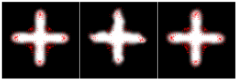
We performed HGM analysis on longitudinal 3D-MRI sequences for seven individuals diagnosed with Alzheimer’s disease with maximum scan range of 5 years. At the individual level of HGM, seven geodesic regressions are performed independently on the time-series of scans. At the group level, the initial conditions of the average geodesic are estimated based on the estimated initial conditions of seven individuals at individual level. The naive serial implementation of this algorithm took 7.5 hours to run 500 iterations of gradient descent for optimization on this dataset. Figure 5 reports the estimated initial conditions for the group geodesic at age=66 for different level of noise variance in intercept and slope terms.

Fig. 5.

Estimated group geodesics initial conditions for 3D MRI using HGM. Left column: σ_S >> σ_I, does not represent average trend. Right column: σ_I = 0.1, σ_S = 0.1, better representative of the average trend. For fair comparison same cut-off was used for visualization of deformation momenta on both the runs.

We observe that forcing both the image and momenta to match the corresponding initial conditions of individual geodesics results in a different estimate of initial conditions for the group geodesic when compared to ignoring the momenta and forcing the image matching alone. For higher variance on the momenta matching term (${\sigma }_S^2\to \infty$), the resulting deformation directions exhibit patterns of deformation across the whole brain (Figure 5, Left). This is because variability across the subjects is very high. These deformations are capturing variability in brain shape across the population more than representing an average trajectory within an individual and hence is not a representative of the longitudinal trend in the population.

On the other hand, lowering the variance in the momenta matching term (ρ_S = 0.1, ρ_I = 0.1, Figure 5, Right) results in deformation patterns around regions expected to be changing for an individual as time progresses. In particular, the information about individual trajectories are taken into account in the averaging process more than inter-subject variability information, thus resulting in an average shape change that represents the longitudinal trend in the population. This is in accordance with the simple Euclidean case presented earlier (Figure 1), where ignoring the velocity matching results in an average line that does not represent the longitudinal variability in the population and hence fail to represent an average trajectory of changes in the dependent variable.

References

- 1.Arnol’d VI: Sur la géométrie différentielle des groupes de Lie de dimension infinie et ses applications à l’hydrodynamique des fluides parfaits. Ann. Inst. Fourier 16, 319–361 (1966) [Google Scholar]
- 2.Beg M, Miller M, Trouvé A, Younes L: Computing large deformation metric mappings via geodesic flows of diffeomorphisms. IJCV 61(2), 139–157 (2005) [Google Scholar]
- 3.Durrleman S, Pennec X, Trouvé A, Gerig G, Ayache N: Spatiotemporal atlas estimation for developmental delay detection in longitudinal datasets. In: MICCAI pp. 297–304. Springer-Verlag, Berlin, Heidelberg (2009) [DOI] [PMC free article] [PubMed] [Google Scholar]
- 4.Fishbaugh J, Prastawa M, Durrleman S, Piven J, Gerig G: Analysis of longitudinal shape variability via subject specific growth modeling. In: MICCAI pp. 731–738. Springer-Verlag, Berlin, Heidelberg (2012) [DOI] [PMC free article] [PubMed] [Google Scholar]
- 5.Fletcher PT: Geodesic regression on Riemannian manifolds. In: MICCAI Workshop on Mathematical Foundations of Computational Anatomy pp. 75–86 (2011) [Google Scholar]
- 6.Laird NM, Ware JH: Random-effects models for longitudinal data. Biometrics 38(4), pp. 963–974 (1982) [PubMed] [Google Scholar]
- 7.Lorenzi M, Ayache N, Frisoni GB, Pennec X: Mapping the Effects of Ab142 Levels on the Longitudinal Changes in Healthy Aging: Hierarchical Modeling Based on Stationary Velocity Fields. In: MICCAI 2011 Springer, Heidelberg (2011) [DOI] [PubMed] [Google Scholar]
- 8.Miller MI, Trouvé A, Younes L: Geodesic shooting for computational anatomy. Journal of Mathematical Imaging and Vision 24(2), 209–228 (2006) [DOI] [PMC free article] [PubMed] [Google Scholar]
- 9.Muralidharan P, Fletcher P: Sasaki metrics for analysis of longitudinal data on manifolds. In: IEEE Conference on CVPR pp. 1027–1034 (june 2012) [DOI] [PMC free article] [PubMed] [Google Scholar]
- 10.Niethammer M, Huang Y, Vialard FX: Geodesic regression for image time-series. In: MICCAI 2011, vol. 6892, pp. 655–662. Springer Berlin Heidelberg (2011) [DOI] [PMC free article] [PubMed] [Google Scholar]
- 11.Singh N, Hinkle J, Joshi S, Fletcher PT: A vector momenta formulation of diffeomorphisms for improved geodesic regression and atlas construction. In: International Symposium on Biomedial Imaging (ISBI) (April 2013) [DOI] [PMC free article] [PubMed] [Google Scholar]
- 12.Younes L, Arrate F, Miller MI: Evolution equations in computational anatomy. Neuroimage 45(1 Suppl), S40–S50 (2009) [DOI] [PMC free article] [PubMed] [Google Scholar]