PROBING IN VIVO MICROSTRUCTURE WITH T₁-T₂ RELAXATION CORRELATION SPECTROSCOPIC IMAGING

Abstract

Quantitative MR relaxometry can provide unique subvoxel information about the microscopic tissue compartments that are present in a large imaging voxel. However, unambiguously distinguishing between these tissue compartments continues to be challenging with conventional methods due to the illposedness of the inverse problem. This paper describes a new imaging approach, which we call T₁ Relaxation-T₂ Relaxation Correlation Spectroscopic Imaging (RR-CSI), that uses two-dimensional relaxation encoding combined with spatially-constrained reconstruction to help overcome illposedness. Results are shown with real data, including what we believe to be the first in vivo demonstration of multidimensional relaxation correlation spectroscopic imaging.

1. INTRODUCTION

Imaging microscopic tissue features is very important for a number of biomedical applications, but is difficult to do directly with conventional MRI due to practical limits on spatial resolution. For example, in vivo human scans are often limited to millimeter-scale voxels. To avoid resolution limits, modern microstructure MRI methods often represent each voxel as a partial volume mixture of multiple tissue micro-compartments, and use contrast encoding methods to distinguish and unmix the different sub-voxel components.

Multicomponent relaxation imaging [1–3] represents one such form of microstructure imaging, and leverages the fact that MR relaxation parameters like T₁, T₂, and $T_2^{\ast }$ are sensitive to microscopic biochemical tissue features and vary between different tissue compartments of interest. The basic idea of the approach is to generate a 1D “spectrum” for each voxel of an MR image, where each spectrum describes the distribution of the relaxation parameter values (for a given parameter of interest) that coexist with the corresponding voxel. This results in a spectroscopic image that contains both spatial and spectral dimensions, and whose spectral peaks can be integrated along the spectral dimension to generate spatial maps corresponding to different microscopic tissue compartments. For example, myelin water imaging [1] is a multicomponent relaxation method that is used to estimate a fractional map of the microscopic myelin water compartment within the brain.

However, estimating multiple relaxation parameters within a single voxel is equivalent to the estimation of multi-exponential decays, and is a classically ill-posed problem. In part due to this ill-posedness, modern 1D relaxation imaging methods that only encode a single relaxation parameter are not currently able to separate all of the different tissue microstructural compartments that are known to exist within a voxel. In this work, we describe a new approach to microstructure imaging that uses 2D relaxation encoding of both the T₁ and T₂ relaxation parameters along with spatially-constrained estimation of the high-dimensional spectroscopic image. This new approach, which we call T₁ Relaxation-T₂ Relaxation Correlation Spectroscopic Imaging (RR-CSI), has substantially enhanced capabilities for mapping of microstructural compartments. While we have reported a preliminary description of RR-CSI in a very recent conference [4], this paper will present the first in vivo RR-CSI spatial maps of microscopic tissue compartments.

Our new RR-CSI approach is motivated in part by previous 2D relaxation approaches [5–9], w2hich Ref. [7] names as relaxation-relaxation correlation spectroscopy (RR-COSY). These RR-COSY methods have been shown to provide much better compartment resolution capabilities than 1D relaxation encoding approaches. However, while some of these existing approaches have acquired spatially-resolved imaging data, they have either focused on voxel-by-voxel or volume-averaged spectrum estimation, and unlike our new RR-CSI approach, have never been used for in vivo spatial mapping.

In addition, our new RR-CSI approach is also motivated by our recent introduction of diffusion-relaxation correlation spectroscopic imaging (DR-CSI) [10]. DR-CSI was a fundamentally new approach to correlation spectroscopic imaging that used spatially-constrained estimation to enable the first demonstration of spatial mapping in the context of diffusion-relaxation spectroscopy. DR-CSI uses a similar 2D contrast encoding experiment to RR-CSI and has similar inverse problem structure, but makes use of different contrast mechanisms that may be sensitive to different aspects of the tissue microstructure. As we were developing DR-CSI, we made the key observation that while voxel-by-voxel 2D spectrum estimation is easier than voxel-by-voxel 1D spectrum estimation, it is still a difficult ill-posed inverse problem. As a result, 2D spectrum estimation still generally required a large number of high SNR measurements to obtain good results. On the other hand, inspired by theoretical observations from [11], we realized that spatial-spectral modeling of the data and spatially-constrained estimation of a spectroscopic image could substantially improve the posedness of the inverse problem. The incorporation of spatially-constrained estimation into DR-CSI was a major breakthrough that enabled high-quality spatial maps to be derived from much less and lower-quality data than were required by previous methods that used voxel-by-voxel or volume-averaged spectrum estimation.

Our new RR-CSI approach combines the contrast encoding ideas from RR-COSY with the spatial-spectral modeling and spatially-constrained estimation ideas of DR-CSI. Compared to previous approaches, RR-CSI enables high-quality multidimensional spectroscopic images to be derived from a relatively small number of data samples, which makes it practical enough for us to apply to in vivo human subjects. As our results will demonstrate, the RR-CSI approach has the potential to provide powerful new insight into the microscopic compartments within biological tissues.

2. DESCRIPTION OF RR-CSI

Without loss of generality (see [4] for a more general description), we will describe RR-CSI for an inversion-recovery spin echo experiment. In this context and assuming no exchange, the ideal noiseless data acquisition model is given by

$$m(x,y,TI,TE)=\iint f(x,y,T_1,T_2)(1-2e^{-T1/T_1})e^{-TE/T_2}d{T}_{1}d{T}_2,$$ (1)

where (x, y) are the spatial coordinates, m(x, y, TI, TE) is the measured data acquired with contrast encoding parameters TI (inversion time) and TE (echo time), and f(x, y, T₁, T₂) is the unknown 4D spectroscopic image that we wish to estimate.

Given this signal model, RR-CSI seeks to estimate f(x, y, T₁, T₂) under the constraints that we want to estimate a spectroscopic image that is both nonnegative (a classical constraint within the RR-COSY literature [5–9]) and spatially smooth (to substantially improve the conditioning of spectrum estimation [10, 11]). Practically, we perform this estimation procedure by solving a dictionary-based spatially-regularized nonnegative least squares optimization problem. In particular, we use a dictionary of different T₁ and T₂ values to generate a discretized approximation of Eq. (1):

$${\mathbf{\text{m}}}_n={\mathbf{\text{Kf}}}_n\text{ for }n=1,\dots ,N.$$ (2)

In writing this expression, we assume that data is collected for P distinct combinations of the contrast encoding parameters TI and TE, represented as (TI_p, TE_p) for p = 1, …,P; we assume that a measured image with N voxels is generated for each set of contrast encodings, and that there is one-toone voxel correspondence between different contrasts; we use ${\mathbf{\text{m}}}_n\in {ℝ}^P$ to denote the data vector corresponding to the nth voxel, containing all P of the measured contrasts; we assume that we have chosen a set of Q discrete T₁ and T₂ combinations to represent our dictionary, represented as (T1_q, T2_q) for q = 1, …,Q; we use $\mathbf{\text{K}}\in {ℝ}^{P\times Q}$ to denote the dictionary matrix with entries ${\left[\mathbf{\text{K}}\right]}_{pq}=(1-2e^{-T{I}_p/T{1}_q})e^{-T{E}_p/T{2}_q}$; and we use ${\mathbf{\text{f}}}_n\in {ℝ}^Q$ is to denote the vector of samples of the multidimensional spectrum for the nth voxel. Note that the ill-posedness of 2D spectrum estimation arises because the columns of the K matrix are formed from exponential decays and are highly correlated with one another.

Our proposed RR-CSI approach estimates the spectroscopic image by solving the following optimization problem:

$${\left\{{\widehat{\mathbf{\text{f}}}}_n\right\}}_{n=1}^N=\underset{{\left\{{\mathbf{\text{f}}}_n\right\}}_{n=1}^N}{\arg \min }\sum _{n=1}^N\left[t_n{\Vert {\mathbf{\text{m}}}_n-{\mathbf{\text{kf}}}_n\Vert }_2^2+\text{λ}\sum _{j\in {\Delta }_n}{\Vert {\mathbf{\text{f}}}_j-{\mathbf{\text{f}}}_n\Vert }_2^2\right]$$ (3)

subject to the constraints that f_n > 0 for n = 1, …,N, with the vector inequality interpreted elementwise. In this expression, λ is a regularization parameter that controls the strength of the spatial smoothness constraint, Δ_n is the index set for the spatial neighborhood of the nth voxel, and t_n is a binary mask used to avoid fitting multidimensional correlation spectra to noise-only voxels of the image (t_n = 1 if the nth voxel is inside the object, and otherwise t_n = 0). This is a simple convex optimization problem which we can solve globally using standard techniques. We obtained solutions using an in-house MATLAB program that implements an alternating directions method of multipliers algorithm, as described in our previous work [10].

3. RESULTS

We have performed extensive simulation and experimental testing of RR-CSI, but for brevity, only present two different illustrative experimental results. The following subsections describe RR-CSI of a small pumpkin and RR-CSI of an in vivo human brain.

3.1. Small Pumpkin

We acquired real RR-CSI data of a small pumpkin using an inversion recovery Carr-Purcell-Meiboom-Gill (CPMG) sequence on a 3T human MRI system (Achieva; Philips Health-care, Best, The Netherlands) with 2 mm × 2 mm in-plane resolution, 4 mm slice thickness, and TR = 5000 ms. For simultaneous T₁ and T₂ contrast encoding, we used every combination of 7 inversion times (TI = 0, 100, 200, 400, 700, 1000, and 2000 ms) and 15 echo times (from TE = 7.5 ms to 217.5 ms in 15 ms increments) for a total of P = 105 contrasts. A high-resolution (0.5 mm × 0.5 mm) image of the same slice was also acquired for reference.

For estimation, a dictionary K was constructed with Q = 10, 000 dictionary elements. Optimization was performed using λ = 0.01 and zero initialization.

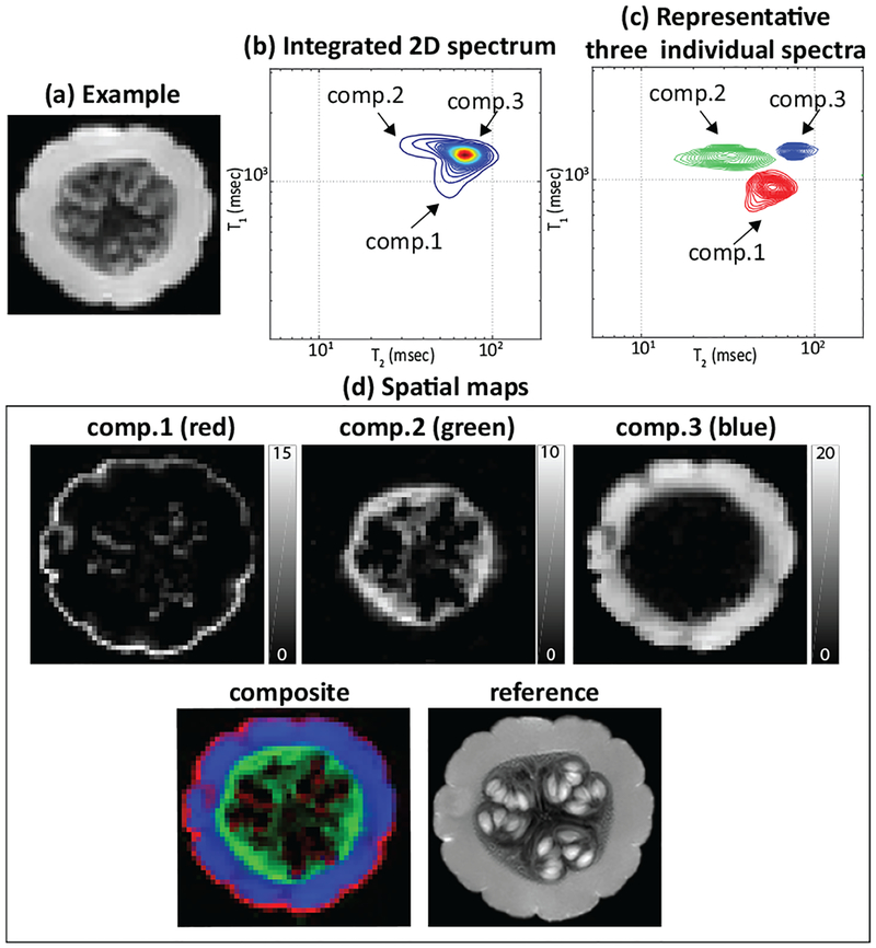
Results are shown in Fig. 1. As can be seen in Fig. 1(b,c), we observe one strong peak and two weaker peaks in the integrated spectrum. By integrating these peaks, we can generate the spatial maps shown in Fig. 1(d). While there is no ground truth in this case, the compartments we have estimated are consistent with our knowledge about the anatomy of a pumpkin, and are also consistent with the high-resolution features we are able to see from the reference image. Due to space constraints, we have not shown spatially-varying spectra derived from our estimated spectroscopic image. However, these spatially varying spectra clearly identify the presence of partial voluming between these three compartments.

Fig. 1:

RR-CSI of the pumpkin. (a): An example image from the full data set (TI=0 ms, TE=7.5 ms). (b): The average 2D RR-CSI spectrum (integrated over all voxels). (c): Three representative individual spectra plotted from different spatial locations. (d): (top) Spatial maps of the three peaks, (bottom-left) the composite image where each component is color-coded (red: comp.1, green: comp.2, and blue: comp.3), and (bottom-right) the high-resolution reference image.

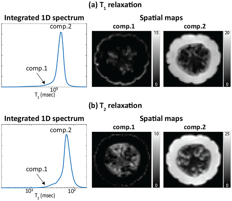
For comparison of our approach against 1D methods, we also performed two different kinds of 1D relaxation spectrum estimation. Specifically, 1D T₁ relaxation spectra were estimated for each voxel from the seven different TIs at TE = 7.5 ms, and and 1D T₂ relaxation spectra were estimated for each voxel from the fifteen different TEs. For improved results, the 1D spectroscopic images were both estimated using spatial constraints and the cost function from Eq. (3). Results are shown in Fig. 2. Note that the three spectral peaks that are clearly separated in 2D are not easily separated in either of the 1D cases. As a result, the 1D cases fail to successfully separate as many compartments as RR-CSI.

Fig. 2:

Estimation results from (a) conventional 1D T₁ relaxation encoding and (b) conventional 1D T₂ relaxation encoding. Each figure shows (left) the estimated spectra integrated across all voxels, and (right) spatial maps of the integrated spectral peaks from the estimated spectroscopic image.

3.2. In vivo human brain

In vivo human brain data was acquired using the same imaging protocol and sequence parameters from the pumpkin experiment, except that we did not use any data with TE=7.5 ms. This resulted in a total of P = 98 contrast encodings. It is worth noting that this single-slice RR-CSI dataset was acquired within 20 minutes, which is feasible for in vivo applications.

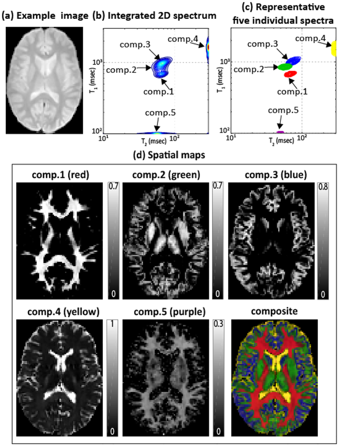
The spectroscopic image was estimated using the same reconstruction parameters as for the pumpkin, and results are shown in Fig. 3. In this case, we observed five resolved peaks. These five peaks closely match with anatomical expectations: component 1 seems to correspond to a part of white matter (WM); component 2 seems to correspond to a mixture of WM and gray matter (GM); component 3 seems to correspond to gray matter (GM); component 4 seems to correspond to cerebrospinal fluid (CSF); and component 5 resembles the myelin water compartment identified in previous literature [1]. However, it should be noted that the relaxation characteristics of the CSF-like component and the myelin water-like component do not match with the literature values. This discrepancy should be expected, since our experiment design has not been optimized for these components. In particular, our experiment used a relatively short TR, meaning that the slowly-relaxing CSF component is unlikely to fully relax between excitations. In addition, we expect that our inversion times may be too coarsely sampled to accurately estimate the T₁ parameter of myelin water. Nevertheless, we are still able to separate realistic-looking components that seem to correspond to CSF and myelin water. It is important to emphasize that our approach clearly separated out anatomical structures and revealed partial voluming of the associated structure, which is impossible with conventional 1D methods. Results from another slice of the same brain (not shown due to space constraints) are consistent with those from Fig. 3.

Fig. 3:

RR-CSI of the human brain. (a): An example image from the full data set (TI=0 ms, TE=22.5 ms). (b): The average 2D RR-CSI spectrum (integrated over all voxels). (c): Five representative individual spectra plotted from different spatial locations. (d): Spatial maps (represented as fractions so that they add to one) of the five peaks, along with the color-coded composite image (red: comp.1, green: comp.2, blue: comp.3, yellow: comp.4, and purple: comp.5).

Importantly, the ability to identify 5 distinct compartments with RR-CSI is a substantial performance improvement over previous 1D approaches based on T₂ spectra [1, 3] that usually only separate 2 or 3 compartments.

4. CONCLUSION

RR-CSI is a novel approach to imaging microstructure that uses high-dimensional contrast encoding together with high-dimensional spatial-spectral image reconstruction. In this paper, we described and evaluated RR-CSI, and demonstrated in vivo results for the first time. We believe that this approach reveals information that has not been easy accessible with traditional approaches, and has the potential to enable substantially more informative experiments in both basic research and clinical applications.