A Bayesian Approach for 4D Flow Imaging of Aortic Valve in a Single Breath-hold

Abstract

Purpose:

To develop and validate a data processing technique that allows phase-contrast MRI-based 4D flow imaging of the aortic valve in a single breath-hold.

Theory and Methods:

To regularize the ill-posed inverse problem, we extend a recently proposed 2D phase-contrast MRI method to 4D flow imaging. Adopting an empirical Bayes approach, spatial and temporal redundancies are exploited via sparsity in the wavelet domain, and the voxel-wise magnitude and phase structure across encodings is captured in a conditional mixture prior that applies regularizing constraints based on the presence of flow. We validate the proposed technique using data from a mechanical flow phantom and five healthy volunteers.

Results:

The flow parameters derived from the proposed technique are in good agreement with those derived from reference datasets for both in vivo and mechanical flow experiments at accelerations rates as high as R = 27. Additionally, the proposed technique outperforms kt SPARSE-SENSE and a method that exploits spatio-temporal sparsity but does not utilize signal structure across encodings.

Conclusion:

Using the proposed technique, it is feasible to highly accelerate 4D flow acquisition and thus enable aortic valve imaging within a single breath-hold.

Introduction

Alterations in hemodynamics have been linked to wide-ranging cardiovascular conditions. Phase-contrast (PC)-MRI is an established imaging technique that enables non-invasive mapping of hemodynamics (1, 2). For PC-MRI, the encoding can be performed over a volume, across the cardiac cycle, and for all three directional components of the velocity vector, providing spatially and temporally resolved mapping of the blood velocity vector. This technique is often termed as “4D flow imaging,” and it permits evaluation of three-directional hemodynamics within three-dimensional vasculature across the cardiac cycle (3). Because of impractically long acquisition times associated with 4D flow imaging, clinical application of PC-MRI is generally limited to planar imaging with a single velocity encoding direction. The accuracy of such an approach is sensitive to the placement of the imaging plane and the misalignment of the velocity encoding direction with respect to the blood flow direction (4), resulting in underestimation of the flow and velocity and, in turn, potential misclassification of disease severity. In contrast, 4D flow imaging, with its volumetric coverage and ability to capture all three components of the velocity, avoids some of the potential measurement errors associated with planar imaging.

In PC-MRI, velocity information is encoded into the phase of the complex-valued image. In the case of 4D flow, the 3D k-space at each cardiac phase is sampled multiple times, each time with a different set of velocity encoding gradients. At least four different velocity encodings are required to encode the nuisance reference phase as well as the phases corresponding to three-directional flow. As a result, the acquisition time for 4D flow imaging can be excessively long, with scan times exceeding 30 minutes (3). These long scan times make 4D flow imaging less cost effective, introduce artifacts related to change in physiology or patient motion, and make the acquisition process stressful for patients.

A number of techniques have been developed to accelerate PC-MRI. Parallel MRI (pMRI), which employs multiple receive coils, has been shown to provide two to three-fold acceleration for PC-MRI (5). State-of-the-art methods to accelerate PC-MRI often combine randomized sampling, pMRI, and image recovery inspired by compressed sensing. For 2D imaging, Kim et al. proposed kt SPARSE-SENSE that combines randomized sampling, pMRI, and sparsity of temporal principal components, yielding a six-fold acceleration to measure portal and hepatic venous flow (6). Kwak et al. recovered five-fold accelerated 2D PC-MRI by enforcing total variation (TV) minimization of both encoded and compensated images as well as exploiting the sparsity of the complex difference between the compensated and encoded images (7). Knobloch et al. proposed a method that utilizes both temporal principal component analysis and the complex difference of velocity encoded and velocity compensated images to report an eight-fold acceleration for 4D flow imaging (8). More recently, Sun et al. employed both sparsity and partial separability constraints to achieve an acceleration rate of eight for 4D flow imaging (9), and Tan et al. enforced equality of magnitudes between the encoded and compensated images and utilized radial sampling to achieve a temporal resolution of 36 ms (10).

In this work, we describe an empirical Bayes approach for inversion of highly accelerated 4D flow data. A novel contribution that characterizes this work is a Bayesian model that, in addition to spatio-temporal sparsity, exploits the spatially varying dependencies in magnitude and phase across an arbitrary number of velocity encoded images. The resulting problem is made computationally tractable by a combination of standard and loopy belief propagation, leading to a novel iterative inversion algorithm. The framework, called ReVEAL4D, is a non-trivial extension of our recently described 2D PC-MRI technique referred to as Reconstructing Velocity Encoded MRI with Approximate message passing aLgorithms (ReVEAL) (11). ReVEAL4D is validated using in vivo and mechanical phantom data, yielding acceleration rates in access of twenty.

Theory

Notation

For this work, bold symbols will be used to represent vectors and matrices, with matrices capitalized, e.g., y = Ax to represent the vector matrix product. Elements from a matrix will be represented as a_ij for the j^th column and i^th row of A, and x_i for the i^th element of a vector x. In the case where the vector contains a subscript, the notation x_bi will represent the i^th element of vector x_b. The symbol × will represent element-wise multiplication when used with vectors. Let I_n denote the n-by-n identity matrix. Lastly, the notation $\mathcal{C}\mathcal{N}$ (x; μ, σ²) will be used to represent a circularly symmetric complex Gaussian distribution for the random variable x with mean μ and variance σ². The same notation is adopted for jointly Gaussian random vectors.

Signal model

We adopt a similar signal model to the one presented in (11) with the 2D operators replaced with their 3D equivalents. Noiseless k-space data ${\tilde{\mathit{y}}}_i^{k,t}$ from the k^th receive coil, t^th frame, and i^th velocity encoding are expressed as

$${\tilde{\mathit{y}}}_i^{k,t}={\mathit{D}}_i^t\mathcal{F}{\mathit{S}}_i^{k,t}{\mathit{\rho }}_i^t,$$ [1]

where ${\mathit{D}}_i^t$ is a k-space sampling selection operator, $\mathcal{F}$ is the 3D Fourier operator, and ${\mathit{S}}_i^{k,t}$ is a diagonal matrix that represents 3D coil sensitivity map. Here, ${\mathit{\rho }}_i^t\in {ℂ}^N$ is a vectorization of the three-dimensional image to be recovered, ${\tilde{\mathit{y}}}_i^{k,t}\in {ℂ}^M$ is the vector of noiseless Fourier measurements. The signal representing all coils and time indices is denoted as

$${\tilde{\mathit{y}}}_i={\mathit{A}}_i{\mathit{\rho }}_i,$$ [2]

where i represents different velocity encodings. In this work, we assume i ∈ {b, x, y, z} where b, x, y, and z represent compensated reference, x-encoded, y-encoded, and z-encoded measurements, respectively.

Bayesian data model

We adopt a Bayesian modeling approach to the inversion task. Probabilistic models are formulated to describe: the relationship of the measured data to the unknown image sequences, the relationships among the four encoded image sequences, and the compressibility of the four 3D spatio-temporal sequences. The modeling assumptions, which are approximate but physically motivated, provide a flexible and effective means to incorporate prior knowledge for the purpose of regularizing the inverse problem. To begin, we define the magnitudes and phases of the complex-valued reference, x-encoded, y-encoded, and z-encoded images (12):

$${\mathit{\rho }}_b={\mathit{m}}_b\times e^{j\left({\mathit{\theta }}_b\right)}$$ [3]

$${\mathit{\rho }}_x={\mathit{m}}_x\times e^{j\left({\mathit{\theta }}_b+{\mathit{\theta }}_x\right)}$$ [4]

$${\mathit{\rho }}_{\mathit{y}}={\mathit{m}}_y\times e^{j\left({\mathit{\theta }}_b+{\mathit{\theta }}_y\right)}$$ [5]

$${\mathit{\rho }}_z={\mathit{m}}_z\times e^{j\left({\mathit{\theta }}_b+{\mathit{\theta }}_z\right)}$$ [6]

where ρ_b is the complex-valued reference (velocity compensated) image, θ_b is the reference phase, and m_b is the reference magnitude. Here, the x-, y- and z-encoded signals have magnitudes m_x, m_y, and m_z, respectively, and velocity encoded phases θ_x, θ_y, and θ_z, respectively. Each measurement is observed under the following model

$${\mathit{y}}_i={\mathit{A}}_i{\mathit{\rho }}_i+{\varphi }_i,\forall i=b,x,y,z.$$ [7]

Here y_b, y_x, y_y, and y_z are the noisy reference, x-encoded, y-encoded, and z-encoded k-space measurements, respectively. The additive noise signals φ_b, φ_x, φ_y, and φ_z are described by zero mean circularly symmetric complex Gaussian distributions with variance ω². Finally, we introduce a Bernoulli indicator, v ∈ {0,1}^N, to denote the non-zero velocity locations in the image, i.e., where θ_x, θ_y, or θ_z is nonzero.

By application of Bayes’ rule and independence of the additive noise across encodings, the posterior distribution of the unknown parameters conditioned on the measurements is given by

$$\begin{gathered} p\left({\mathit{\rho }}_b,{\mathit{\rho }}_x,{\mathit{\rho }}_y,{\mathit{\rho }}_z,{\mathit{\theta }}_x,{\mathit{\theta }}_y,{\mathit{\theta }}_z,\mathit{v}|{\mathit{y}}_b,{\mathit{y}}_x,{\mathit{y}}_y,{\mathit{y}}_z\right)\propto \\ p\left({\mathit{\rho }}_b,{\mathit{\rho }}_x,{\mathit{\rho }}_y,{\mathit{\rho }}_z,{\mathit{\theta }}_x,{\mathit{\theta }}_y,{\mathit{\theta }}_z,\mathit{v}\right) \\ \times p\left({\mathit{y}}_b|{\mathit{\rho }}_b\right)p\left({\mathit{y}}_x|{\mathit{\rho }}_x\right)p\left({\mathit{y}}_y|{\mathit{\rho }}_y\right)p\left({\mathit{y}}_z|{\mathit{\rho }}_z\right). \end{gathered}$$ [8]

Since the additive noise terms are Gaussian, it follows that the likelihood terms in Eq. [8] are given by

$$p\left({\mathit{y}}_i|{\mathit{\rho }}_i\right)=\mathcal{C}\mathcal{N}\left({\mathit{y}}_i;{\mathit{A}}_i{\mathit{\rho }}_i,{\omega }^2\mathit{I}\right),\forall i=b,x,y,z.$$ [9]

To complete the model requires choice of the prior. By application of the chain rule for probability density functions, the prior can be factorized as follows.

$$\begin{gathered} p\left({\mathit{\rho }}_b,{\mathit{\rho }}_x,{\mathit{\rho }}_y,{\mathit{\rho }}_z,{\mathit{\theta }}_x,{\mathit{\theta }}_y,{\mathit{\theta }}_z,\mathit{v}\right)=p\left({\mathit{\rho }}_b\right)p(\mathit{v}|{\mathit{\rho }}_b)p\left({\mathit{\theta }}_x|{\mathit{\rho }}_b,\mathit{v}\right) \\ \times p\left({\mathit{\theta }}_y|{\mathit{\rho }}_b,\mathit{v},{\mathit{\theta }}_x\right)p\left({\mathit{\theta }}_z|{\mathit{\rho }}_b,\mathit{v},{\mathit{\theta }}_x,{\mathit{\theta }}_y\right)p\left({\mathit{\rho }}_x|{\mathit{\rho }}_b,\mathit{v},{\mathit{\theta }}_x,{\mathit{\theta }}_y,{\mathit{\theta }}_z\right) \\ \times p\left({\mathit{\rho }}_y|{\mathit{\rho }}_b,\mathit{v},{\mathit{\theta }}_x,{\mathit{\theta }}_y,{\mathit{\theta }}_z,{\mathit{\rho }}_x\right)p\left({\mathit{\rho }}_z|{\mathit{\rho }}_b,\mathit{v},{\mathit{\theta }}_x,{\mathit{\theta }}_y,{\mathit{\theta }}_z,{\mathit{\rho }}_x,{\mathit{\rho }}_y\right). \end{gathered}$$ [10]

The resulting distributions in Eq. [10] are difficult to model, and the graph drawn using these distributions would contain tight loops, greatly increasing the computational complexity needed to solve the graph. To avoid these difficulties, we make simplifying conditional independence assumptions to yield tractable message passing, while still capturing salient physical dependencies that provide a regularizing capability for the inverse problem. The simplified prior is given as

$$\begin{gathered} p\left({\mathit{\rho }}_b,{\mathit{\rho }}_x,{\mathit{\rho }}_y,{\mathit{\rho }}_z,{\mathit{\theta }}_x,{\mathit{\theta }}_y,{\mathit{\theta }}_z,\mathit{v}\right)\approx p\left({\mathit{\rho }}_b\right)p(\mathit{v})p\left({\mathit{\theta }}_x\right)p\left({\mathit{\theta }}_y\right) \\ \times p\left({\mathit{\theta }}_z\right)p\left({\mathit{\rho }}_x|{\mathit{\rho }}_b,{\mathit{\theta }}_x,\mathit{v}\right)p\left({\mathit{\rho }}_y|{\mathit{\rho }}_b,{\mathit{\theta }}_y,\mathit{v}\right)p\left({\mathit{\rho }}_z|{\mathit{\rho }}_b,{\mathit{\theta }}_z,\mathit{v}\right). \end{gathered}$$ [11]

The x-, y-, and z-encoded images are assumed to be conditionally independent given the reference image, e.g., $p\left({\mathit{\rho }}_z|{\mathit{\rho }}_b,\mathit{v},{\mathit{\theta }}_x,{\mathit{\theta }}_y,{\mathit{\theta }}_z,{\mathit{\rho }}_x,{\mathit{\rho }}_y\right)=p\left({\mathit{\rho }}_z|{\mathit{\rho }}_b,{\mathit{\theta }}_z,\mathit{v}\right)$. The advantages of these conditional independence assumptions in Eq. [11] are two-fold. First, the resulting posterior factor graph takes on a tree-like structure that avoids loops, which greatly reduces the computational complexity of the algorithm. Second, the resulting Generalized Approximate Message Passing (GAMP) prior can be further simplified to a two-component mixture that has tractable message derivations and computation. As described in (11), we choose the following conditional prior on each complex-valued voxel:

$$p\left({\rho }_{in}|{\rho }_{bn},{\theta }_{in},v_n\right)=\left(1-v_n\right)\mathcal{C}\mathcal{N}\left({\rho }_{in};{\rho }_{bn},{\sigma }^2\right)+v_n\mathcal{C}\mathcal{N}\left({\rho }_{in};{\rho }_{bn}{e}^{j{\theta }_{in}},{\sigma }^2\right)\forall i=x,y,z.$$ [12]

Here, n =1, 2,..., N is the voxel index, and v_n, ρ_in, ρ_bn, and θ_in represent n^th elements of v,ρ_i, ρ_b, and θ_i, respectively. Eq. [12] expresses a spatially varying dependency between encoded and compensated voxels. For a voxel with flow (v_n = 1), only magnitude similarity is enforced between encoded and compensated images; for a voxel with no-flow (v_n = 0), both magnitude and phase similarities are enforced between encoded and compensated images. The variance σ² > 0 is used to allow for potential mismatch in the measured data compared to the idealized assumptions in Eq. [3–6].

The unknown velocity indicator variable, v, is also treated as an unknown and is jointly inferred along with other parameters. Since the presence of flow at each voxel is likely to be sustained across adjacent frames, we further regularize the problem by enforcing a temporal prior of a steady-state Markov chain on v. Let $v_n^t$ be the velocity indicator variable at spatial location n at time t; then

$$p\left(v_n^t|v_n^{t-1}=1\right)={\left(1-p_{01}\right)}^{v_n^t}{\left(p_{01}\right)}^{1-v_n^t}$$ (13)

$$p\left(v_n^t|v_n^{t-1}=0\right)={\left(\frac{\delta p_{01}}{1-\delta }\right)}^{v_n^t}{\left(1-\frac{\delta p_{01}}{1-\delta }\right)}^{1-v_n^t}$$ (14)

$$p_{01}\triangleq p\left(v_n^t=0|v_n^{t-1}=1\right)$$ (15)

$$\delta \triangleq p\left(v_n^t=1\right).$$ (16)

The parameters δ and p₀₁ for the Markov chain are learned from the data via expectation maximization (EM) from the GAMP approximate posteriors as described here (13). To remove loops on the graph, we use separate indicator variables v_x, v_y, and v_z to represent velocity in the x-, y- and z-encoded images. For the velocity encoded phase, i.e., p(θ_x), p(θ_y), and p(θ_z), we choose a non-informative prior with uniform density on the interval [0, 2π). Finally, instead of postulating a prior on the image pixels themselves, we choose an analysis compressed sensing formulation (14) and apply a complex-valued Laplace prior on the wavelet coefficients, i.e., s

$$p\left({\mathit{\rho }}_i\right)\propto \prod _{j=1}^N{\left(\frac{\lambda }{2\pi }\right)}^2{e}^{-\lambda \left|{\left[\mathbf{\Psi }{\mathit{\rho }}_i\right]}_j\right|}\forall i=b,x,y,z,$$ [17]

where ${\left[\mathbf{\Psi }{\mathit{\rho }}_i\right]}_j$ is the j^th coefficient under 3D spatio-temporal sparsifying transform Ψ.

We use the term ReVEAL4D to describe the integrated approach that exploits spatially varying magnitude and phase structure unique to 4D flow imaging, utilizes image compressibility in the non-decimated wavelet domain, and employs message passing computation to recover 4D flow images from highly under-sampled data. For comparison, we also evaluate the performance of L1-SENSE and kt SPARSE-SENSE (6). Both ReVEAL4D and L1-SENSE utilize the same wavelet penalty, sampling pattern, and message passing computation; however, L1-SENSE (15) reconstructs each of the four encoded images independently and therefore does not exploit any regularizing relationships among the encoded images - a distinguishing feature of ReVEAL4D. In contrast to ReVEAL4D and L1-SENSE, kt SPARSE-SENSE, when extended to 4D flow imaging, does not utilize spatial sparsity but exploits sparsity of the temporal principal components when all four velocity encodings are concatenated.

Message passing computation

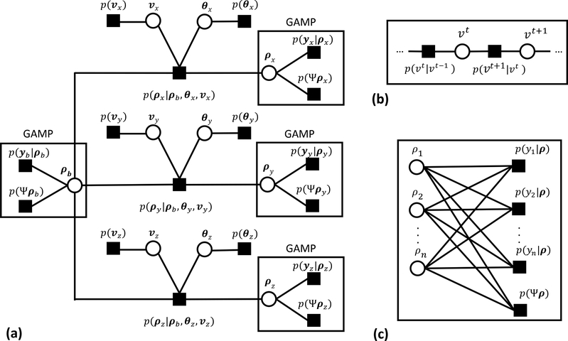
The posterior distribution in Eq. [8] is visualized as the factor graph in Fig. 1. By applying belief propagation, we approximately compute the posterior marginal distributions for ρ_b, ρ_x, ρ_y, ρ_z, θ_b, θ_x, θ_y, θ_z, and v. For the non-loopy portions of the graph, a single forward and backward pass is sufficient to find a solution. However, each of the likelihood terms creates loops in the graph. For these portions, we apply the GAMP algorithm which uses central limit theorem and Taylor series approximations to greatly reduce the computational complexity (16). The GAMP algorithm is a generalization of the approximate message passing algorithm (AMP) (17) to arbitrary measurement matrices and output channel distributions. The algorithm proceeds in three phases. First, update the messages in the loopy portions of the graph with GAMP and no input prior. Second, use the approximate messages from GAMP and standard belief propagation to update the input priors for each GAMP sub-block. Third, iterate each GAMP block with the new input prior. Repeat steps two and three until convergence.

Figure 1:

A factor graph provides a visualization of the Bayesian modeling used for regularized inversion. The reconstruction algorithm is constructed via message passing on the graph and results in an iterative thresholding procedure. (a) The complete graph of the approximate posterior in Eq. [8] in compact vector notation. (b) The subgraph defining the Markov random chain prior on the velocity indicator, v, where v_t represents a given pixel at time point t. (c) The loopy subgraph describing the likelihood terms in Eq. [8]. These loopy portions of the graph are computed using Generalized Approximate Message Passing (GAMP).

The resulting GAMP prior, derived from the graph in Figure 1, for each encoded image is an eight component mixture. Seven of the eight components contain a product of Bessel functions. Due to the presence of the product of Bessel functions, the required GAMP message updates, consisting of the mean and variance of this prior, are difficult or impossible to describe exactly. As such, we apply two simplifications to the GAMP prior to yield tractable update rules. The first approximation reduces the number of mixture components from eight to two. The second approximates the product of three Rician distributions as again a Rician. The resulting approximate prior for an encoded image is give in Appendix A.

Methods

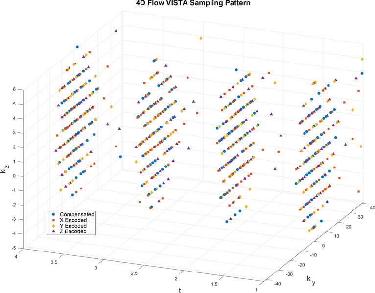
To design an informative k-space sampling pattern, D^t, we extend VISTA sampling patterns (18). VISTA forms variable density, constrained, incoherent sampling patterns by minimizing the Riesz energy on a Cartesian grid. Constraints on the pseudo-random VISTA patterns include: equal samples per time frame; a bound on excursions in k-space, to limit eddy currents; and fully sampled k-space when averaged across time frames. The third of these constraints facilitates estimation of the unknown coil sensitivity maps. We extend the VISTA strategy to jointly design the sampling pattern across a 4D grid consisting of two phase encoding, one temporal, and one velocity encoding dimensions; the third spatial encoding dimension is fully sampled via frequency encoding. An example VISTA pattern over a 4D grid is given in Figure 2, where each marker shape represents a different velocity encoding.

Figure 2:

An example VISTA sampling pattern optimized over the 4D grid consisting of two phase encoding dimensions, k_y and k_z, one time dimension (cardiac frame, t), and one velocity encoding dimension. For visualization, the four velocity encodings are represented by distinct symbols, and only four time frames are shown. To enforce partial Fourier, k_y < −24 was not sampled.

Retrospectively undersampled phantom data

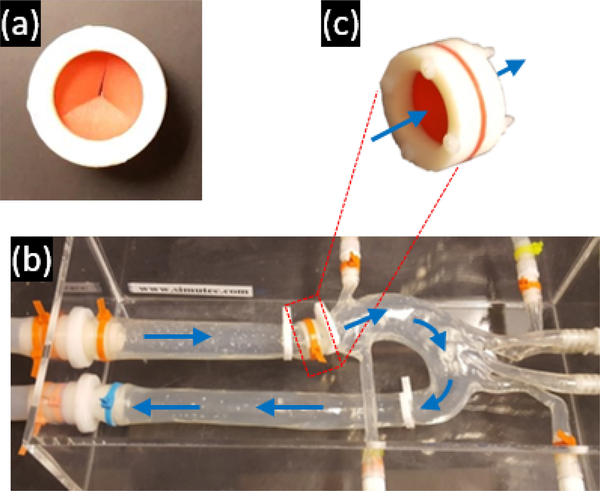
To validate ReVEAL4D, a flow phantom was constructed consisting of an aortic arch phantom and a CardioFlow 5000 MR flow pump (Shelley Medical Imaging Technologies, Toronto, Ontario, Canada). To simulate conditions in vivo, a synthetic valve, shown in Figure 3, was inserted into the aortic arch phantom. The valve consisted of a thin rubber membrane held between two plastic rings. A Y-shaped opening was cut into the membrane to mimic a tricuspid aortic valve. To secure the membrane in place, the two rings were connected together using nylon screws.

Figure 3:

The mechanical flow phantom and valve used in this work. (a) The valve consists of a rigid outer ring and a flexible rubber membrane with opening that mimics the tricuspid aortic valve. (b) The aortic arch phantom with fluid flow direction depicted by arrows. (c) The location and orientation of the valve within the aortic phantom.

All data were collected on a 1.5 T scanner (MAGNETOM, Avanto, Siemens Healthcare, Erlangen, Germany) with an 18-channel cardiac array. A total of four fully sampled datasets were acquired with slightly different flow settings. For the first dataset, collected with isotropic spatial resolution, the volumetric field-of-view (FOV) was oriented such that the readout direction was parallel to the length of the aorta and hence the nominal flow direction. The scan parameters for this data provided isotropic resolution: TE 2.27 ms, TR 4.46 ms, temporal resolusion 36 ms, and VENC 420 cm/s, matrix size 192 × 84 × 30, FOV 402 × 176 × 62 mm, 2.1 mm isotropic resolution, acquisition time 21 minutes, and flip angle 10°. The second through fourth datasets were collected with anisotropic spatial resolution and the readout direction was rotated 75°, 90°, and 105°, respectively, resulting in a nominal flow approximately perpendicular to the largest face of the imaging volume. For datasets 2–4, the scan parameters were: TE 2.27 ms, TR 4.46 ms, temporal resolusion 36 ms, VENC 420 cm/s in the dominant flow direction, VENC 300 cm/s for the remaining two directions, matrix size 168 × 84 × 20, FOV 400 × 175 × 60 mm, a spatial resolution of 2.4 × 2.1 × 3.0 mm³, acquisition time 14 minutes, and flip angle 10°. The data were retrospectively downsampled by acceleration rates R = 8, 10, 12, 14, 16, 18, 20, 22, 24, 26, 28, and 30. All datasets were acquired using a spoiled gradient echo pulse sequence and prospectively triggered segmented acquisition with referenced four-point encoding.

Prospectively undersampled in vivo data

To further test the efficacy of ReVEAL4D, 4D flow data were collected from five healthy volunteers with Imaging slab placed perpendicular to the aorta, centering at the aortic valve. Two 4D acquisitions were acquired per volunteer. The first was a reference scan using respiratory navigator GRAPPA acquisition with an acceleration factor of R = 3. The second scan was a single breath-hold acquisition using VISTA sampling with acceleration rate R between 20 and 27, depending on the FOV. All 4D flow data were collected using a 1.5 T scanner (MAGNETOM, Avanto, Siemens Healthcare, Erlangen, Germany) and an 18-channel cardiac array. The 4D flow data were collected using prospectively triggered segmented acquisition with referenced four-point encoding. Through plane resolution was 6 mm. Eight slices with 50% oversampling were acquired for a total of twelve slices, with a usable slab thickness of 48 mm. Depending on the patient size, the acquisition matrix was 160 × 108 × 12, 144 × 96 × 12, or 128 × 84 × 12. From these three options, the smallest acquisition matrix that yielded in-plane resolution of ≤ 3 mm was selected. The resulting in plane resolutions for all 5 volunteers were 2.2 × 2.9 mm², 2.4 × 2.8 mm², 2.4 × 2.8 mm², 2.3 × 2.9 mm², and 2.3 × 3.0 mm². Further scan parameters were as follows: TE 2.4 ms, TR 4.6 ms, two views per segment yielding a total of eight readouts per cardiac phase in each heartbeat, temporal resolution 36 ms, VENC 130–180 cm/s, and flip angle 10°. The acquisition time for reference datasets ranged from 8 to 14 minutes, while the acquisition time for the accelerated datasets was fixed at 24 heartbeats. In addition, to test the repeatability of ReVEAL4D, ten identical datasets were collected and processed from a sixth volunteer.

Image reconstruction and quantitative evaluation

For the phantom data, the images were reconstructed using ReVEAL4D, kt SPARSE-SENSE after it was extended to 4D flow imaging, and L1-SENSE with retrospective downsampling, and the reference was based on fully sampled data. For the four phantom datasets, a volume of interest (VOI) was hand selected downstream from the synthetic valve to extract flow parameters. All pixels in the VOI resided within the aortic arch and in close vicinity of the valve. Within the VOI, one plane was selected to compute volume flow rate (VFR) per frame, stroke volume (SV), and peak velocity (PV). For PV, the search was performed across all frames. To compare ReVEAL4D, kt SPARSE-SENSE, and L1-SENSE to reference, SV, PV, and normalized mean-squared error (NMSE) were computed across different acceleration rates. NMSE is defined by

$$\text{NMSE}=10\log \left(\frac{{\Vert {\mathit{x}}_{\text{ref}}-\widehat{\mathit{x}}\Vert }_2^2}{\Vert {\mathit{x}}_{\text{ref}}{\Vert }_2^2}\right),$$ [18]

where x_ref is the noisy reference image from fully sampled data and $\widehat{\mathit{x}}$ is the reconstructed image from accelerated data.

For the in vivo data, the images were reconstructed using ReVEAL4D, kt SPARSE-SENSE, and L1-SENSE, and the reference was based on GRAPPA reconstruction from rate-3 dataset collected with respiratory navigators. To extract flow parameters, a VOI was manually selected downstream but in the vicinity of the aortic valve. Within the VOI, the values of SV and PV were computed at four parallel, adjacent slices. ReVEAL4D and L1-SENSE were compared using Bland-Altman analysis, which was performed from twenty (five volunteers, four planes) SV and PV measurements.

Reconstruction algorithms were implemented in custom Matlab (Mathworks, Natick, MA) software running on a Windows 7 PC with a Tesla K40c (Nvidia, Santa Clara, CA). All reconstructions were performed off-line. The coil sensitivity maps were estimated by time-averaging the k-space data and applying the adaptive array combination method (19). The k-space noise variance, ω², was estimated from a 200–240 ms pre-scan data. For faster computation, the 18 measurement coils were compressed to 12 virtual coils (20). For ReVEAL4D and L1-SENSE, 4D (x-y-z-t) wavelet transform had 16 sub-bands. The first sub-band (LLLL), where L represents low frequency, is usually not sparse and was not regularized; the next seven “spatial” sub-bands (***L) were give a relative weight of λ₀, and the last eight “temporal” sub-bands (***H), where H represents high frequency, were given a relative weight of 10λ₀. The global regularization weight, λ₀, was hand-tuned using one flow phantom dataset at R = 12 acceleration and held constant across all datasets and all accelerations. The parameter σ² was set to 1% of the maximum image magnitude, and γ_n (i.e., the prior probability that v_n = 0) was learned via expectation maximization for every n as a function of δ and p₀₁ in Eq. [13–16]. Codes to perform ReVEAL4D reconstruction are provided on Github¹, and codes for the GAMP algorithm are provided here ².

Results

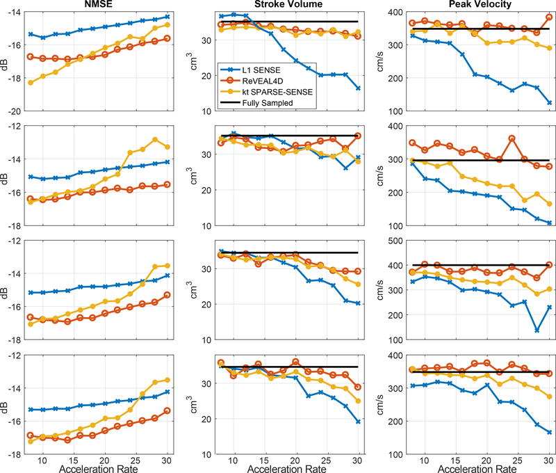
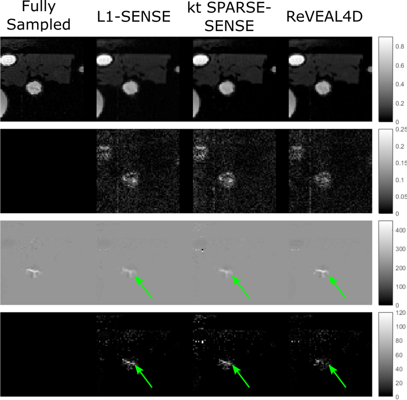
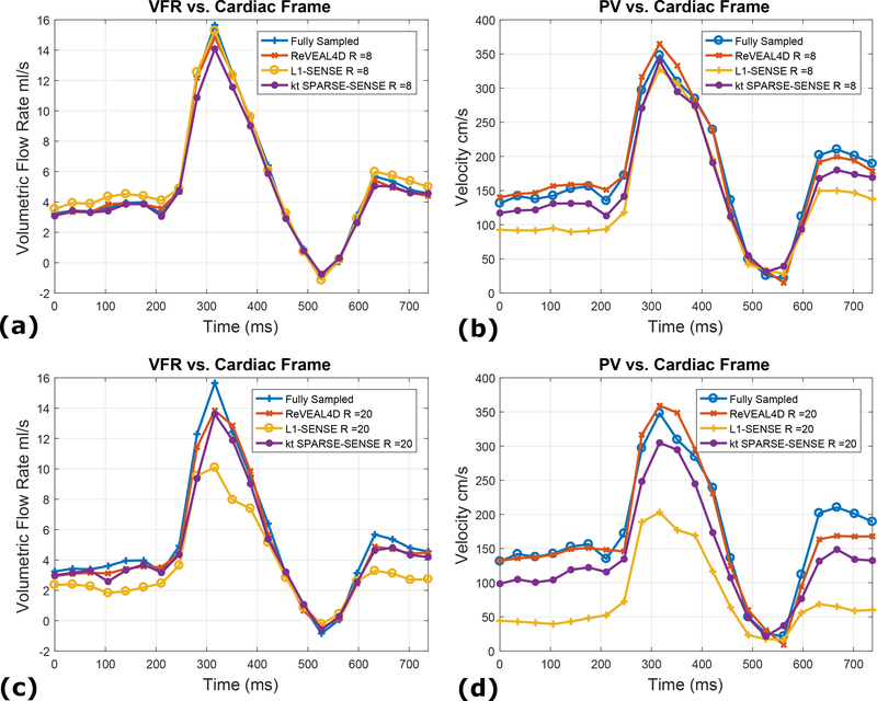
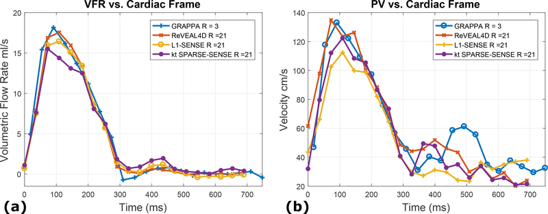
For the phantom data, image quality metrics‒NMSE, SV, and PV‒are displayed in Figure 4; these metrics, for all four datasets, are plotted as function of R. In addition, representative images from fully sampled reference, ReVEAL4D, kt SPARSE-SENSE, and L1-SENSE for acceleration rate R = 20 are shown in Figure 5. Related time-resolved images comparing reference, ReVEAL4D, kt SPARSE-SENSE, and L1-SENSE are included as a movies Supporting Video S1 (R = 8) and Supporting Video S2 (R = 20). To further examine the fidelity of accelerated images, Figure 6 shows representative VFR and PV profiles for two acceleration rates (R = 8 and R = 20).

Figure 4:

Image quality metrics computed from retrospectively accelerated data. ReVEAL4D, kt SPARSE-SENSE, and L1-SENSE are compared to fully sampled data. NMSE, stroke volume, and peak velocity are plotted versus acceleration rate, R. Each row depicts results from one of the four datasets. Each column presents a given quality metric.

Figure 5:

Example images selected from the 4D flow data. ReVEAL4D, kt SPARSE-SENSE, and L1-SENSE are compared to fully sampled data. The first row contains the normalized magnitude images. The second row contain the absolute difference in magnitude between the fully sampled data and accelerated images. The third row contains the velocity maps (cm/s). The fourth row displays the absolute difference between the fully sampled velocity maps and reconstructed velocity maps. Images were reconstructed at an acceleration rate R = 20.

Figure 6:

Representative flow profiles comparing fully sampled data to accelerated data reconstructed with ReVEAL4D, kt SPARSE-SENSE, and L1-SENSE. (a) The VFR per frame for an acceleration rate R = 8. (b) The PV per frame for an acceleration rate R = 8. (c) The VFR per frame for an acceleration rate R = 20. (d) The PV per frame for an acceleration rate R = 20.

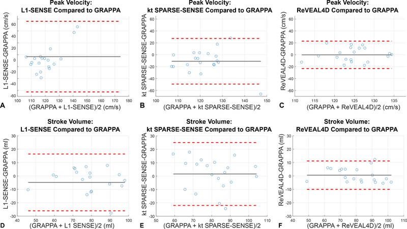
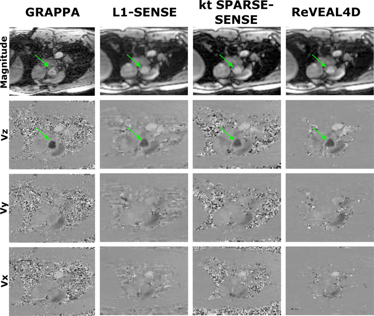
For in vivo data, Bland-Altman analyses were performed for PV and SV and shown in Figure 7. In Figure 8, representative images from GRAPPA, ReVEAL4D, kt SPARSE-SENSE, and L1-SENSE are compared. Related time-resolved images comparing reference, ReVEAL4D, kt SPARSE-SENSE, and L1-SENSE are included as Supporting Video S3. Representative flow profiles for in vivo data are shown in Figure 9. The results from the reproducibility study of ReVEAL4D are provided in Supporting Figure S1, which compares PV and SV across 10 acquisitions of prospectively accelerated datasets. The positive impact of employing Markov chain to regularize v is illustrated in Supporting Figure S2.

Figure 7:

Bland-Altman analyses comparing ReVEAL4D, kt SPARSE-SENSE, and L1-SENSE data acquired in a single breath-hold to respiratory navigator GRAPPA acquisition. Peak velocity and stroke volume were computed in the volume of interest for 4 slices above the aortic valve. (a) Peak velocity recovered using L1-SENSE compared to GRAPPA. (b) Peak velocity computed using kt SPARSE-SENSE compared to GRAPPA. (c) Peak velocity computed using ReVEAL4D compared to GRAPPA. (d) Stroke volume recovered with L1-SENSE compared to GRAPPA. (e) Stroke volume recovered with kt SPARSE-SENSE compared to GRAPPA. (f) Stroke volume recovered using ReVEAL4D compared to GRAPPA.

Figure 8:

Comparison of various 4D flow acquisition techniques in vivo. The first column contains images reconstructed using GRAPPA for respiratory navigator based acquisition and acceleration R = 3. The second, third and fourth columns contain images reconstructed from the same prospectively accelerated acquisition using VISTA sampling with R = 21. The second column contains images reconstructed using L1-SENSE. The third column contains images reconstructed using kt SPARSE-SENSE. The fourth column contains images reconstructed using ReVEAL4D.

Figure 9:

Representative flow profiles for in vivo data, comparing GRAPPA reference data (R = 3) to accelerated data reconstructed with ReVEAL4D, kt SPARSE-SENSE, and L1-SENSE. (a) The VFR per frame for an acceleration rate R = 21. (b) The PV per frame for an acceleration rate R = 21.

For the phantom data, offline reconstruction required approximately 20 minutes for ReVEAL4D and 8 minutes for L1-SENSE. These reconstruction times were accomplished by using Matab GPU support and single precision floating point arithmetic. Most of the increase in runtime is due to ReVEAL4D requiring more iterations to converge versus L1-SENSE. The computation time for kt SPARSE-SENSE, which did not utilize GPU computation, was 5 hours.

Discussion

The Bayesian imaging approach in ReVEAL4D allows for a data model that exploits the unique structure of PC-MRI. The signal structure present between encodings is exploited in ReVEAL4D using a non-Gaussian mixture density, which significantly reduced both bias and variance in the estimated flow parameters; thus, the approach extends the classical use of a regularization penalty, such as L1-norm of wavelet transform coefficients, to exploit a richer set of relationships present among the unknown quantities. Additionally, the conditional mixture density provides a “soft” constraint on the magnitudes among encodings, in contrast to strict equality of magnitudes proposed in other regularization techniques (10). Compared to our previous Bayesian modeling approach for 2D PC-MRI (11), ReVEAL4D also enforces temporal continuity on v using EM-tuned Markov random chain (Eq. [16]) and employs a GAMP prior that regularizes magnitude and phase structure across four velocity encodings (Appendix A).

For the phantom data, ReVEAL4D consistently outperforms L1-SENSE in terms of NMSE by approximately 1.5 dB across all acceleration rates (Figure 4). The performance of ReVEAL4D is comparable to kt SPARSE-SENSE at low acceleration rates; however, at high acceleration rates, ReVEAL4D outperforms kt SPARSE-SENSE by approximately 2 dB. For SV and PV quantification, ReVEAL4D and L1-SENSE perform similarly at acceleration rates R < 16. For R = 18 and above, ReVEAL4D shows consistently better performance over L1-SENSE for both SV and PV quantification. The performance of kt SPARSE-SENSE, in terms of SV and PV quantification, resides between that of ReVEAL4D and L1-SENSE. For ReVEAL4D, both SV and PV quantification error stayed below 20% across all acceleration rates. Images from an example frame at R = 20 are shown in Figure 5, with kt SPARSE-SENSE and L1-SENSE showing significantly increased error in the region of high-velocity jet around the valve. This temporal blurring from L1-SENSE is also evident from Figure 6. At R = 8, ReVEAL4D, kt SPARSE-SENSE, and L1-SENSE recover the VFR profile with high fidelity; however, for PV, the ReVEAL4D reconstruction tracks the fully sampled data more closely. At the higher acceleration rate of R = 20, L1-SENSE shows significant blurring of VFR and severe underestimation of PV, and kt SPARSE-SENSE also shows underestimation of PV. In contrast, ReVEAL4D shows only slight blurring in both VFR and PV.

For in vivo data, the Bland-Altman analyses indicates that ReVEAL4D yields lower bias and narrower limits of agreement compared to L1-SENSE and kt SPARSE-SENSE. For ReVEAL4D, the maximum discrepancy with respect the reference was 18% for PV and 15% for SV. In contrast, for L1-SENSE, the maximum discrepancy with respect the reference was 42% for PV and 27% for SV. Likewise, for kt SPARSE-SENSE, the maximum discrepancy with respect the reference was 36% for PV and 33% for SV. Figure 8 also shows that ReVEAL4D, kt SPARSE-SENSE, and L1-SENSE, compared to GRAPPA, exhibit noise suppression albeit at the cost of visible image blurring. The blurring can be attributed to the high acceleration rate and the resulting lack of data, requiring the acceleration techniques to rely heavily on the regularization compared the data fidelity constraint. The ReVEAL4D images, however, exhibit lesser blurring and more well-defined valve opening. Note, the GRAPPA reference itself contains significant noise, which may be responsible for some of the flow quantification discrepancy between GRAPPA and other methods. Supporting Figure S1 shows the repeatability of ReVEAL4D in a healthy volunteer. For the ten datasets collected back-to-back, the standard deviation in the quantification of PV and SV was 6.0% and 2.6%, respectively.

We identify several limitations of our work. First, our claim of enabling 4D flow imaging in a single breath-hold may not apply to all applications or for all parameter settings. For example, performing 4D flow imaging of the entire aortic arch or performing aortic valve imaging at isotropic resolution of 3 mm or better would not be feasible in a single breath-hold even at acceleration rates of 20 to 27. Second, the results presented in this work focus on two physiological parameters-peak velocity and stroke volume-that are relevant to clinical diagnosis of aortic valve disease. It is, however, not evident if the highly accelerated images generated by ReVEAL4D possess the quality to extract other advanced parameters, including wall shear stress, pulse wave velocity, turbulence intensity, helicity, and 3D pressure gradients. It is likely that extraction of these advanced parameters would require higher overall image quality and spatial resolution. Note, ReVEAL4D can deliver higher imaging quality at the cost of longer acquisition time if breath-holding is not a requirement. Third, ReVEAL4D, like other regularization-based methods, has tuning parameters that can impact the image quality. These parameters include the regularization weights for wavelet bands and the parameter, σ², that controls the variance of the two-component mixture. In this work, we manually optimized these parameters using an additional phantom dataset; the results from this dataset were not included. Once selected, the parameter values were not adjusted on per-dataset basis. Although it is possible that these parameters become highly sub-optimal for a certain experimental setup, ReVEAL4D, being a Bayesian approach, offers the opportunity to automatically tune these parameters using EM methods. Fourth, computation time for ReVEAL4D is long. By using Matlab GPU support, the runtime has been reduced by a factor of 9 over CPU computation; however, the reconstruction time of 20 min for ReVEAL4D may still not be practical in all clinical settings. Yet, there are further opportunities to reduce the runtime either by using multiple GPUs or by further optimizing the code. Fifth, despite realism in the phantom flow dynamics, with peak velocity in excess of 300 cm/s, and in vivo data from a small cohort of healthy subjects, it is not guaranteed if ReVEAL4D will be able to achieve equally high acceleration rates in patients with aortic valve stenosis due to high velocity jets and turbulent flow. Sixth, we have made a simplifying assumption of conditional independence (Eq. [11]) to make ReVEAL4D computationally efficient. By making this assumption, we may have forfeited additional regularization benefits. Seventh, for the in vivo study, we compare breath-held scans with a respitory gated free-breathing reference. Due to pysiological differences between free-breathing and breath-hold states of the cardiopulmonary system, the hemodynamics between the scans could be slightly different. The presented phantom study, however, does not suffer from this limitation. Finally, it is likely that a fraction of patients with valve disease would not be able to hold their breath for 20 s. Despite these limitations, some of which will be investigated in future studies, ReVEAL4D is a promising technique that has a potential to facilitate highly accelerated 4D flow exams in clinic. Also, we believe that there is a room to further shorten the breath-hold. For example, the oversampling of 50% may not be necessary if eSPIRiT based coil-sensitivity maps, which are more tolerant to reduced FOV (21), are used. Also, the breath-holding time can be reduced by 33% by degrading the temporal resolution from 36 ms to 54 ms, which may be adequate in some applications. Even for applications where ReVEAL4D cannot generate results in a single breath-hold, it would be possible to combine ReVEAL4D with prospective or retrospective respiratory gating to enable a free-breathing 4D flow scan that is 5 to 10 fold faster compared to rate-2 GRAPPA.

Conclusion

We have presented an accelerated imaging procedure for phase-contrast MRI-based 4D flow imaging. The procedure has been demonstrated at 1.5T using data from a realistic aortic flow phantom and in vivo data from healthy volunteers. The proposed approach, ReVEAL4D, combines optimized k-space sampling, Bayesian signal modeling, and iterative message passing to regularize the inversion problem for highly under-sampled data. Quantitative flow parameters, including peak velocity and stroke volume, were recovered within 20% of reference values at acceleration rates up to 27, with part of the discrepancy attributable to physiological variations and noise in the reference dataset.

Supplementary Material

Supporting Video S1:

Time-resolved images selected from the 4D flow data. ReVEAL4D, kt SPARSE- SENSE, and L1-SENSE, reconstructed at an acceleration rate R = 8, are compared to fully sampled data. The first row contains the normalized magnitude images. The second row contain the absolute difference in magnitude between the fully sampled data and accelerated images. The third row contains the velocity maps (cm/s). The fourth row displays the absolute difference between the fully sampled velocity maps and reconstructed velocity maps.

Supporting Video S2:

Time-resolved images selected from the 4D flow data. ReVEAL4D, kt SPARSE- SENSE, and L1-SENSE, reconstructed at an acceleration rate R = 20, are compared to fully sampled data. The first row contains the normalized magnitude images. The second row contain the absolute difference in magnitude between the fully sampled data and accelerated images. The third row contains the velocity maps (cm/s). The fourth row displays the absolute difference between the fully sampled velocity maps and reconstructed velocity maps.

Supporting Video S3:

Comparison of various 4D flow acquisition techniques in vivo. The first column contains time-resolved images reconstructed using GRAPPA for respiratory navigator based acquisition and acceleration R = 3. The second, third, and fourth column contain time-resolved images reconstructed from the same prospectively accelerated acquisition using VISTA sampling with R = 21. The second column contains images reconstructed using L1-SENSE. The third column contains images reconstructed using kt SPARSE-SENSE. The fourth column contains images reconstructed using ReVEAL4D.

Appendix A

In this section, we describe the prior used for each GAMP block in Figure 1. Each prior depends on the posterior means and variances estimated from the other three GAMP blocks. For brevity, we adopt a short hand notation for Rician distributions as

$$R(\rho ;\eta ,\alpha )=\frac{|\rho |}{\pi {\alpha }^2}\exp \left(-\frac{|\rho {|}^2+{\eta }^2}{{\alpha }^2}\right)I_0\left(\frac{2|\rho |\eta }{{\alpha }^2}\right)$$ [19]

where I₀(·) represents the zeroth order, modified Bessel function of the first kind. We drop the subscript n and note that the following distributions are for a single voxel. From the message passing updates, the prior for a background encoded voxel, ρ_b, is given by

$$\begin{gathered} p\left({\rho }_b\right)=\left[\mathcal{C}\mathcal{N}\left({\rho }_b;{\tau }_x,{\alpha }_x^2\right)+R\left({\rho }_b;{\tau }_x,{\alpha }_x^2\right)\right]\left[\mathcal{C}\mathcal{N}\left({\rho }_b;{\tau }_y,{\alpha }_y^2\right)+R\left({\rho }_b;{\tau }_y,{\alpha }_y^2\right)\right]\left[\mathcal{C}\mathcal{N}\left({\rho }_b;{\tau }_z,{\alpha }_z^2\right)+R\left({\rho }_b;{\tau }_z,{\alpha }_z^2\right)\right] \\ =\mathcal{C}\mathcal{N}\left({\rho }_b;{\tau }_x,{\alpha }_x^2\right)\mathcal{C}\mathcal{N}\left({\rho }_b;{\tau }_y,{\alpha }_y^2\right)\mathcal{C}\mathcal{N}\left({\rho }_b;{\tau }_z,{\alpha }_z^2\right)+\mathcal{C}\mathcal{N}\left({\rho }_b;{\tau }_x,{\alpha }_x^2\right)R\left({\rho }_b;{\tau }_y,{\alpha }_y^2\right)R\left({\rho }_b;{\tau }_z,{\alpha }_z^2\right) \\ +\mathcal{C}\mathcal{N}\left({\rho }_b;{\tau }_x,{\alpha }_x^2\right)\mathcal{C}\mathcal{N}\left({\rho }_b;{\tau }_y,{\alpha }_y^2\right)R\left({\rho }_b;{\tau }_z,{\alpha }_z^2\right)+\mathcal{C}\mathcal{N}\left({\rho }_b;{\tau }_x,{\alpha }_x^2\right)R\left({\rho }_b;{\tau }_y,{\alpha }_y^2\right)\mathcal{C}\mathcal{N}\left({\rho }_b;{\tau }_z,{\alpha }_z^2\right) \\ +R\left({\rho }_b;{\tau }_x,{\alpha }_x^2\right)\mathcal{C}\mathcal{N}\left({\rho }_b;{\tau }_y,{\alpha }_y^2\right)\mathcal{C}\mathcal{N}\left({\rho }_b;{\tau }_z,{\alpha }_z^2\right)+R\left({\rho }_b;{\tau }_x,{\alpha }_x^2\right)R\left({\rho }_b;{\tau }_y,{\alpha }_y^2\right)\mathcal{C}\mathcal{N}\left({\rho }_b;{\tau }_z,{\alpha }_z^2\right) \\ +R\left({\rho }_b;{\tau }_x,{\alpha }_x^2\right)\mathcal{C}\mathcal{N}\left({\rho }_b;{\tau }_y,{\alpha }_y^2\right)R\left({\rho }_b;{\tau }_z,{\alpha }_z^2\right)+R\left({\rho }_b;{\tau }_x,{\alpha }_x^2\right)R\left({\rho }_b;{\tau }_y,{\alpha }_y^2\right)R\left({\rho }_b;{\tau }_z,{\alpha }_z^2\right). \end{gathered}$$ (20)

In Eq. [20], τ and α are the means and variances, respectively, of the Gaussian messages emitted from each GAMP block; for example, the message emitted from the ρ_x block is $\mathcal{C}\mathcal{N}\left({\rho }_x;{\tau }_x,{\alpha }_x^2\right)$. The first of two simplifiying assumptions is to ignore all but the first and last terms of Eq. [20] yielding

$$p\left({\rho }_b\right)=\mathcal{C}\mathcal{N}\left({\rho }_b;{\tau }_x,{\alpha }_x^2\right)\mathcal{C}\mathcal{N}\left({\rho }_b;{\tau }_y,{\alpha }_y^2\right)\mathcal{C}\mathcal{N}\left({\rho }_b;{\tau }_z,{\alpha }_z^2\right)+R\left({\rho }_b;{\tau }_x,{\alpha }_x^2\right)R\left({\rho }_b;{\tau }_y,{\alpha }_y^2\right)R\left({\rho }_b;{\tau }_z,{\alpha }_z^2\right).$$ [21]

The product of Gaussian pdfs is again Gaussian. Therefore, we can rewrite the first term of Eq. [21] as

$$\mathcal{C}\mathcal{N}\left({\rho }_b;{\tau }_x,{\alpha }_x^2\right)\mathcal{C}\mathcal{N}\left({\rho }_b;{\tau }_y,{\alpha }_y^2\right)\mathcal{C}\mathcal{N}\left({\rho }_b;{\tau }_z,{\alpha }_z^2\right)=\mathcal{C}\mathcal{N}\left({\rho }_b;\mu ,{\beta }^2\right)$$ [22]

$$\mu =\frac{{\tau }_x{\alpha }_y^2{\alpha }_z^2+{\tau }_y{\alpha }_x^2{\alpha }_z^2+{\tau }_z{\alpha }_x^2{\alpha }_y^2}{{\alpha }_y^2{\alpha }_z^2+{\alpha }_x^2{\alpha }_z^2+{\alpha }_x^2{\alpha }_y^2}$$ [23]

$${\beta }^2=\frac{{\alpha }_x^2{\alpha }_y^2{\alpha }_z^2}{{\alpha }_y^2{\alpha }_z^2+{\alpha }_x^2{\alpha }_z^2+{\alpha }_x^2{\alpha }_y^2}.$$ [24]

For the second simplifying assumption, we approximate the product of three Rician distributions as again Rician in a similar manner to the Gaussians above, yielding

$$R\left({\rho }_b;{\tau }_x,{\alpha }_x^2\right)R\left({\rho }_b;{\tau }_y,{\alpha }_y^2\right)R\left({\rho }_b;{\tau }_z,{\alpha }_z^2\right)\approx R\left({\rho }_b;\eta ,{\beta }^2\right)$$ [25]

$$\eta =\frac{|{\tau }_x|{\alpha }_y^2{\alpha }_z^2+|{\tau }_y|{\alpha }_x^2{\alpha }_z^2+|{\tau }_z|{\alpha }_x^2{\alpha }_y^2}{{\alpha }_y^2{\alpha }_z^2+{\alpha }_x^2{\alpha }_z^2+{\alpha }_x^2{\alpha }_y^2}.$$ [26]

The resulting approximate prior has a simplified form of

$$p\left({\rho }_b\right)=\gamma R\left({\rho }_b;\eta ,{\beta }^2\right)+(1-\gamma )\mathcal{C}\mathcal{N}\left({\rho }_b;\mu ,{\beta }^2\right)\gamma \in [0,1),$$ [27]

which yields tractable message passing updates and lower computational cost than Eq. [20]. The weight, γ, is learned for each voxel from the data as a function the Markov chain parameters δ and p₀₁, described in Eq. [13–16]. The simplified prior of Eq. [27] may forfeit some regularizing structure compared to the exact description of Eq. [20]. However, the underlying regularization of Eq. [27] admits an easily interpreted meaning. Based on the value of γ, ρ_b is close in magnitude to the variance weighted mean, η, or ρ_b is close in magnitude and phase to the variance weighted mean, μ. Prior distributions for ρ_x, ρ_y, and ρ_z have the same form as Eq. [27], with different μ, β and η. Each encoded image uses means and variances from the remaining three, e.g., ρ_x uses τ_b, τ_y, and τ_z to form μ, β, and η in Eq. [27].

References

- 1.Gatehouse P, Keegan J, Crowe L, Masood S, Mohiaddin R, Kreitner KF, Firmin D. Applications of phase-contrast flow and velocity imaging in cardiovascular MRI. Eur. Radiol 2005; 15:2172–2184. [DOI] [PubMed] [Google Scholar]
- 2.Pelc NJ, Herfkens RJ, Shimakawa A, Enzmann DR. Phase contrast cine magnetic resonance imaging. Magn. Reson. Q. 1991; 7:229–254. [PubMed] [Google Scholar]
- 3.Markl M, Kilner P, Ebbers T. Comprehensive 4D velocity mapping of the heart and great vessels by cardiovascular magnetic resonance. J. Cardiovasc. Magn. Reson. 2011; 13:7. [DOI] [PMC free article] [PubMed] [Google Scholar]
- 4.da Silveira JS, Smyke M, Jin N, Ahmad R, Jafari L, Scandling D, Dickerson JA, Raman SV, Simon-etti OP. Aortic Stenosis assessment with a 3-directional phase contrast magnetic resonance technique. Comparison to transthoracic echocardiography. J. Cardiovasc. Magn. Reson. 2015; 17:1–2.25589308 [Google Scholar]
- 5.Thunberg P, Karlsson M, Wigström L. Accuracy and reproducibility in phase contrast imaging using SENSE. Magn. Reson. Med. 2003; 50:1061–1068. [DOI] [PubMed] [Google Scholar]
- 6.Kim D, Dyvorne HA, Otazo R, Feng L, Sodickson DK, Lee VS. Accelerated phase-contrast cine MRI using k-t SPARSE-SENSE. Magn. Reson. Med. 2012; 67:1054–1064. [DOI] [PMC free article] [PubMed] [Google Scholar]
- 7.Kwak Y, Nam S, Akcakaya M, Basha TA, Goddu B, Manning WJ, Tarokh V, Nezafat R. Accelerated aortic flow assessment with compressed sensing with and without use of the sparsity of the complex difference image. Magn. Reson. Med. 2013; 70:851–858. [DOI] [PMC free article] [PubMed] [Google Scholar]
- 8.Knobloch V, Boesiger P, Kozerke S. Sparsity transform k-t principal component analysis for accelerating cine three-dimensional flow measurements. Magn. Reson. Med. 2013; 70:53–63. [DOI] [PubMed] [Google Scholar]
- 9.Sun A, Zhao B, Ma K, Zhou Z, He L, Li R, Yuan C. Accelerated phase contrast flow imaging with direct complex difference reconstruction. Magn. Reson. Med. 2016;. [DOI] [PMC free article] [PubMed] [Google Scholar]
- 10.Tan Z, Roeloffs V, Voit D, Joseph AA, Untenberger M, Merboldt KD, Frahm J. Model-based reconstruction for real-time phase-contrast flow MRI: Improved spatiotemporal accuracy. Magn. Reson. Med. 2016;. [DOI] [PubMed] [Google Scholar]
- 11.Rich A, Potter LC, Jin N, Ash J, Simonetti OP, Ahmad R. A Bayesian model for highly accelerated phase-contrast MRI. Magn. Reson. Med. 2016; 76:689–701. [DOI] [PMC free article] [PubMed] [Google Scholar]
- 12.Pelc NJ, Bernstein MA, Shimakawa A, Glover GH. Encoding strategies for three-direction phase-contrast MR imaging of flow. J Magn. Reson. Imaging 1991; 1:405–413. [DOI] [PubMed] [Google Scholar]
- 13.Ziniel J, Schniter P. Dynamic compressive sensing of time-varying signals via approximate message passing. IEEE Trans. Signal Process. 2013; 61:5270–5284. [Google Scholar]
- 14.Cands E, Eldar Y, Needell D, Randall P. Compressed sensing with coherent and redundant dictionaries. Applied and Computational Harmonic Analysis 2011; 31:59–73. [Google Scholar]
- 15.Liu B, Zou YM, Ying L. Sparsesense: Application of compressed sensing in parallel mri. In: 2008. International Conference on Information Technology and Applications in Biomedicine, In: 2008 International Conference on Information Technology and Applications in Biomedicine, May 2008 pp. 127–130. [Google Scholar]
- 16.Rangan S Generalized approximate message passing for estimation with random linear mixing. In: Proc. IEEE Int. Symp. Inform. Thy, In: Proc. IEEE Int. Symp. Inform. Thy., Jul 2011 pp. 2168–2172. [Google Scholar]
- 17.Donoho DL, Maleki A, Montanari A. Message-passing algorithms for compressed sensing. Proc. Natl. Acad. Sci. 2009; 106:18914–18919. [DOI] [PMC free article] [PubMed] [Google Scholar]
- 18.Variable density incoherent spatiotemporal acquisition (VISTA) for highly accelerated cardiac MRI. Magn. Reson. Med. 2015; 74:1266–1278. [DOI] [PMC free article] [PubMed] [Google Scholar]
- 19.Walsh DO, Gmitro AF, Marcellin MW. Adaptive reconstruction of phased array MR imagery. Magn. Reson. Med. 2000; 43:682–690. [DOI] [PubMed] [Google Scholar]
- 20.Buehrer M, Pruessmann KP, Boesiger P, Kozerke S. Array compression for MRI with large coil arrays. Magn. Reson. Med. 2007; 57:1131–9. [DOI] [PubMed] [Google Scholar]
- 21.Uecker M, Lai P, Murphy MJ, Virtue P, Elad M, Pauly JM, Vasanawala SS, Lustig M. ESPIRiT-an eigenvalue approach to autocalibrating parallel MRI: Where sense meets grappa. Magnetic Resonance in Medicine 2014; 71:990–1001. [DOI] [PMC free article] [PubMed] [Google Scholar]
Associated Data
This section collects any data citations, data availability statements, or supplementary materials included in this article.
Supplementary Materials